Impact of Stochastic Atmospheric Density on Satellite Orbit Stability

Abstract

The orbit stability of a satellite is a crucial aspect in its design and maintenance. Without an analysis of orbital trajectories, satellites, much like any small celestial objects, are prone to orbital decay, collision with other orbiting objects, or even variations in trajectory, leading to the impossibility of performing their tasks. Starting from an equation of angular momentum variation applied to a satellite in a circular orbit around Earth, the system of second-order ordinary differential equations of motion for the satellite can be determined. By introducing this term into the satellite’s stochastic dynamic system, results much closer to reality are obtained. This paper analyses the accuracy and stability of five finite difference schemes in solving SDEs, applying them to a second-order stochastic differential equation. The uniformity of the stabilisation behaviour in the stochastic trajectories of the stochastic dynamical system is discussed, and the noise impact on the results is analysed by comparing cases with variations in the noise coefficient. The graphical results of the SDEs presented in this paper highlight the symmetry of the stochastic trajectories around the solution of the deterministic system.

1. Introduction

The rotational dynamics of satellites, particularly in Low Earth Orbit (LEO), are significantly influenced by deterministic and stochastic forces. In such orbits, the gravity gradient torque, determined by the uneven distribution of Earth’s gravitational field, plays a dominant deterministic role. However, aerodynamic torques caused by atmospheric drag and magnetic torques from interactions with the magnetic fields of the Earth and the moon are subject to stochastic variability due to fluctuations in atmospheric density and magnetic field strength. These effects are particularly pronounced in LEO, where atmospheric density is higher compared to higher altitudes, amplifying the stochastic influences. Additionally, external factors like solar radiation, meteorite impacts, and Earth’s electric field further contribute to the stochastic nature of satellite motion.

For LEO satellites, moments of inertia are also subject to stochastic variation due to the dynamic effects of thermo-elastic deformations, crew activity, and fluid behaviour within tanks. These complexities make the orbital motion a highly stochastic process, best modelled using stochastic differential equations. This study builds upon foundational research in stochastic modelling and existing research in stochastic orbit analysis, offering insights into the influence of deterministic gravity gradient forces and stochastic aerodynamic torques. By applying stochastic stability techniques, this research provides a comprehensive understanding of satellite dynamics in LEO, highlighting both the opportunities and challenges of operating in such an environment.

The analysis of the stability of an orbit is a calculation of great importance in the design of a satellite or in monitoring its operation, which is related to the field of aerospace engineering and the dynamics of celestial body systems [1]. The importance of maintaining a stable orbit is dictated by the vital role that satellites play in many areas: locating devices equipped with GPS technology and ensuring a safe ground and air navigation system, taking photographs of the Earth’s surface, observing weather conditions and, above all, transmitting and retrieving information to and from Earth via telecommunications.

Deterministic methods of analysing the trajectory of satellites cannot take into account the unpredictable nature of the parameters of the atmosphere or their deviations from the standard model of the atmosphere, such as variations in temperature, pressure, and density (which has the greatest impact on the attitude of the satellites) [2]. Stochastic analysis using stochastic processes adds to the differential equations a probabilistic (or diffusion) term that allows for the integration of random variations [3,4] in the mentioned parameters—density, temperature, and pressure—taking into account the impact that these variations have on the results of the equations and thus obtaining results closer to reality.

Stochastic calculus, a domain that emerged in the early years of the twentieth century, was theorised by the Japanese mathematician Kiyosi Itô [5]. This domain has seen a great rise in interest from researchers in recent years and is greatly utilised in domains involving a certain degree of uncertainty or risk, such as in finance [6,7], meteorology, medicine, epidemiology [8], as well as in engineering, due to the underlying mathematical theory of associating a degree of probability, deviation from the mean, or even uncertainty to a differential equation.

The subject of interest of this paper is the study of the stability of the orbit of an artificial satellite of Earth using finite difference methods in solving the stochastic differential equations of the motion of the satellite and the comparison in stability of five stochastic finite difference schemes (Euler–Maruyama, Milshtein, Stochastic Heun, and two Runge–Kutta schemes).

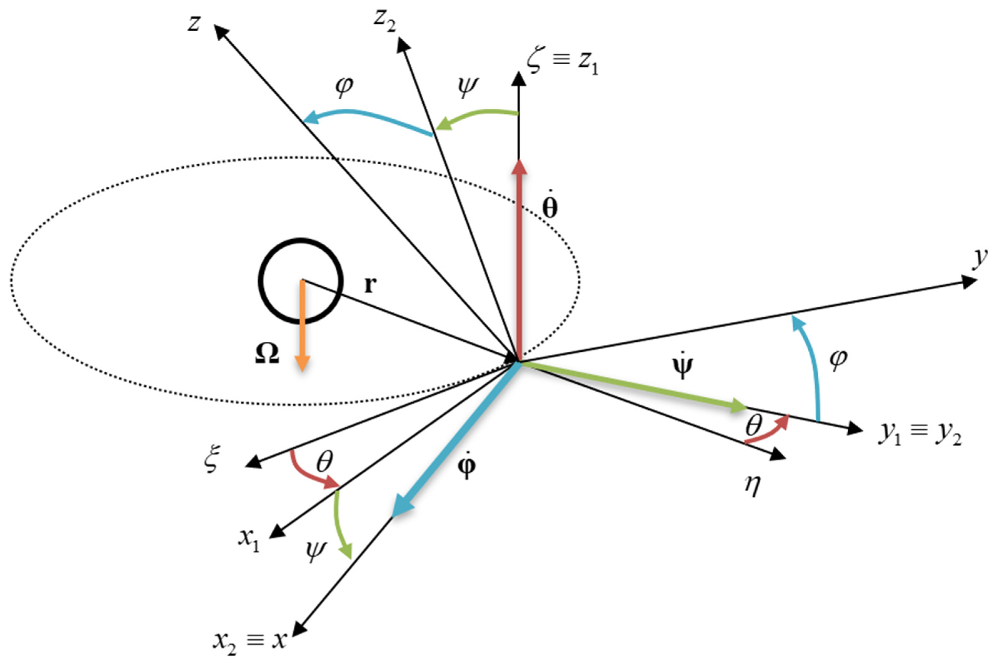
2. Short Review of the Mechanical Aspects of the Satellite

Consider a rigid satellite occupying a spatial domain Λ, with local density ρ, which is orbiting Earth at a constant altitude on a circular equatorialLEO, with a constant angular velocity vector Ω parallel to the vertical axis of the Earth.

The axes system Oξηζ has the origin O positioned in the mass centre of the satellite (for which the position vector in relation to the centre of mass of Earth is r), the Oξ axis tangent to the circular trajectory, and the Oη axis radially positioned and the Oζ axis perpendicular to the trajectory plane. This axes system is, thus, an orbital one, and not a refence system completely “tied” to the satellite. Taking in consideration the fact that the satellite can spin around the mentioned axes, it is appropriate to describe a secondary system of axes, the Oxyz system, with the three axes aligned with the principal axes of the satellite (around which the tensor of inertia is a diagonal matrix [9]):

$$\mathbf{J}=\left(\begin{array}{ccc}\mathrm{A}& 0& 0\\ 0& \mathrm{B}& 0\\ 0& 0& \mathrm{C}\end{array}\right),$$

(1)

in which A, B, and C are the principal moments of inertia. The transformation of coordinates between the two axes systems can be written using Euler transformations [9]:

$$\left(\begin{array}{c}x\\ y\\ z\end{array}\right)={\mathbf{R}}_{1,2,3}\left(\theta ,\psi ,\phi \right)\left(\begin{array}{c}\xi \\ \eta \\ \zeta \end{array}\right),$$

(2)

in which the matrix of rotation is as follows:

$${\mathbf{R}}_{1,2,3}\left(\theta ,\psi ,\phi \right)=\left(\begin{array}{ccc}\cos \theta \cos \psi & \sin \theta \cos \psi & -\sin \psi \\ \cos \theta \sin \psi \sin \phi -\sin \theta \cos \phi & \sin \theta \sin \psi \sin \phi +\cos \theta \cos \phi & \cos \psi \sin \phi \\ \cos \theta \sin \psi \cos \phi +\sin \theta \sin \phi & \sin \theta \sin \psi \cos \phi -\cos \theta \sin \phi & \cos \psi \cos \phi \end{array}\right).$$

(3)

Due to the periodicity of the trigonometric functions, the angles are usually defined in the interval of [0,2π]. However, as we will see in the following sections of this paper, the stochastic stability of the mentioned satellite can be properly studied if the domain is extended to the real numbers set, $\mathbb{R}$, offering the ability to quantify either the instability trait of the motion differential equation or the number of full revolutions before stabilisation. The Euler angles and the position of the mass centre of the satellite are visualised in Figure 1, in which the intermediary reference systems are obtained as follows:

• Reference system Ox₁y₁z₁ is obtained by rotating Oξηζ around axis Oζ with the angular displacement θ.
• Reference system Ox₂y₂z₂ is obtained by further rotating Ox₁y₁z₁ around Oy₁ with the angular displacement ψ.
• Principal reference system Oxyz is obtained by rotating Ox₂ around with the angular displacement φ; the final axis Ox is the symmetry axis of the satellite.

Utilising the corresponding rotation matrices, the total angular velocity of the satellite can be evaluated by the following formulation:

$$\mathbf{\omega }=\left(\begin{array}{c}{\omega }_x\\ {\omega }_y\\ {\omega }_z\end{array}\right)=\left(\begin{array}{c}\dot{\phi }-\left(\dot{\theta }-\Omega \right)\sin \psi \\ \dot{\psi }\cos \phi +\left(\dot{\theta }-\Omega \right)\cos \psi \sin \phi \\ -\dot{\psi }\sin \phi +\left(\dot{\theta }-\Omega \right)\cos \psi \cos \phi \end{array}\right).$$

(4)

As previously mentioned, Ω is the angular speed of the mass centre of the satellite around the mass centre of the Earth. The angular momentum of the satellite can be written, according to the angular displacements and principal moments of inertia A, B, and C, in the absence of linear velocity (since the satellite is only exhibiting a rotational movement), as follows [10]:

$${\mathbf{K}}_{\mathbf{O}}=\left(\begin{array}{c}\mathrm{A}\left[\dot{\phi }-\left(\dot{\theta }-\Omega \right)\sin \psi \right]\\ \mathrm{B}\left[\dot{\psi }\cos \phi +\left(\dot{\theta }-\Omega \right)\cos \psi \sin \phi \right]\\ \mathrm{C}\left[-\dot{\psi }\sin \phi +\left(\dot{\theta }-\Omega \right)\cos \psi \cos \phi \right]\end{array}\right)=\mathbf{J}\mathbf{\omega },$$

(5)

in which J is the tensor of inertia from (1) and $\mathbf{\omega }$ is the total angular velocity defined in (4). Due to the assumption that the satellite is axisymmetric around the Ox axis, we can write A < B = C. One can linearise this formulation (5) and the formulation in (4) considering small angle variations:

$${\sin {\alpha }_i\cong {\alpha }_i\left[\mathrm{rad}\right],\cos {\alpha }_i\cong 1\left[\mathrm{rad}\right], \alpha }_i{\alpha }_j\cong 0, {\alpha }_i{\dot{\alpha }}_j\cong 0, \forall {\alpha }_i\in \left\{\phi ,\psi ,\theta \right\},$$

(6)

so that the total angular velocity and the angular momentum become the following:

$$\mathbf{\omega }\cong \left(\begin{array}{c}\dot{\phi }+\Omega \psi \\ \dot{\psi }-\Omega \phi \\ \dot{\theta }-\Omega \end{array}\right),{\mathbf{K}}_{\mathbf{O}} \cong \left(\begin{array}{c}\mathrm{A}\left(\dot{\phi }+\Omega \psi \right)\\ \mathrm{B}\left(\dot{\psi }-\Omega \phi \right)\\ \mathrm{C}\left(\dot{\theta }-\Omega \right)\end{array}\right)$$

(7)

The total derivative of the angular momentum in (7), considering the definition of the total derivative of a vector field [11], is equal to the sum of all the torques (moments of forces) which act on the satellite [1,9]:

$${\displaystyle \frac{\mathrm{d}{\mathbf{K}}_{\mathbf{O}}}{\mathrm{dt}}}={\displaystyle \frac{\partial {\mathbf{K}}_{\mathbf{O}}}{\partial \mathrm{t}}}+\mathbf{\omega }\times {\mathbf{K}}_{\mathbf{O}}=\sum _i{\mathbf{M}}_{\mathbf{O}}\left({\mathbf{F}}_i\right).$$

(8)

Differentiating partially with respect to time and calculating the cross product between the total angular velocity and angular momentum, the differential of the angular momentum vector can be written as follows:

$${\displaystyle \frac{\mathrm{d}{\mathbf{K}}_{\mathbf{O}}}{\mathrm{dt}}}=\left(\begin{array}{c}\mathrm{A}\ddot{\phi }+{\Omega }^2\left(\mathrm{C}-\mathrm{B}\right)\phi +\Omega \left(\mathrm{A}+\mathrm{B}-\mathrm{C}\right)\dot{\psi }\\ \mathrm{B}\ddot{\psi }+{\Omega }^2\left(\mathrm{C}-\mathrm{A}\right)\psi -\Omega \left(\mathrm{A}+\mathrm{B}-\mathrm{C}\right)\dot{\phi }\\ \mathrm{C}\ddot{\theta }\end{array}\right).$$

(9)

The moments of forces which act on the satellite are the gravity torque and the aerodynamic torque. The gravity torque has the following formulation:

$${\mathbf{M}}_{\mathbf{G}}=\mathrm{k}{\displaystyle \frac{\mathrm{M}}{{\mathrm{R}}^3}}\left(\begin{array}{c}-3\phi \left(\mathrm{C}-\mathrm{B}\right)\\ 0\\ -3\theta \left(\mathrm{A}-\mathrm{B}\right)\end{array}\right),$$

(10)

in which k is the universal gravitational constant (k = 6.6743 × 10⁻¹¹ m³kg⁻¹s⁻² [12,13]), R is the orbit altitude, and M is the mass of the Earth. As a consequence to Binet’s Equation [14] and to the circular orbit, the following equation stands:

$$\mathrm{kM}={\mathrm{R}}^3{\Omega }^2.$$

(11)

In order to simplify the three-dimensional second-order differential equation, one can consider that the yaw and roll angles of the satellite remain constant and equal to zero [1]:

$$\psi \left(t\right)=\phi \left(t\right)\cong 0.$$

(12)

According to the authors in [1,15,16], the aerodynamic torque has the following formulation:

$$\mathbf{M}={\displaystyle \frac{1}{2}}\rho {\mathrm{V}}^2\left[\mathbf{f}\left(\phi ,\psi ,\theta \right)+\mathbf{K}\left(\dot{\phi },\dot{\psi },\dot{\theta }\right)\mathbf{\omega }\right],$$

(13)

where $\rho$ is the local density of the atmosphere, V is the mass centre velocity of the satellite, and f is a vector function of the yaw, roll, and pitch angles, which depends on the satellite geometry and which determines the restoring aerodynamic torque. In the case of the constant roll and yaw angles [1], this vector has the following form:

$$\mathbf{f}=\left(\begin{array}{c}0\\ 0\\ -{\mathrm{S}}_0{\mathrm{L}}_0{\mathrm{c}}_1\theta \end{array}\right).$$

(14)

Moreover, K is a matrix function of the angular velocities, which determines the dissipative term of the aerodynamic torque, and, for the same hypotheses, the product between K and the total angular velocity vector $\mathbf{\omega }$ takes the form [1]:

$$\mathbf{K}\mathbf{\omega }=\left(\begin{array}{c}0\\ 0\\ -{\mathrm{S}}_0{\mathrm{L}}_0{\mathrm{c}}_2{\displaystyle \frac{\mathrm{d}\theta }{\mathrm{dt}}}\end{array}\right).$$

(15)

Finally, the aerodynamic torque for the case of constant roll and yaw angles [1] for an axisymmetric satellite that has only one component on the Oz axis (pitch axis) [1,15,16,17]:

$${\mathbf{M}}_{\mathrm{A}}\cong {\displaystyle \frac{\rho {\mathrm{V}}^2}{2}}\left[\left(\begin{array}{c}0\\ 0\\ -{\mathrm{S}}_0{\mathrm{L}}_0{\mathrm{c}}_1\theta \end{array}\right)+\left(\begin{array}{c}0\\ 0\\ -{\mathrm{S}}_0{\mathrm{L}}_0{\mathrm{c}}_2{\displaystyle \frac{\mathrm{d}\theta }{\mathrm{dt}}}\end{array}\right)\right],$$

(16)

where ${\mathrm{S}}_0{ \mathrm{and} \mathrm{L}}_0$ are reference area and length of the satellite, c₁ is a unitless coefficient, and c₂ is a coefficient with the S.I. unit of seconds. To take into account the unpredictable external factors that can disturb the equilibrium of the satellite [1,2,18], in Equation (14), we introduced the Wiener process to the atmospheric density [1]:

$$\rho ={\rho }_0\left(1+\epsilon {\displaystyle \frac{\mathrm{dW}}{\mathrm{dt}}}\right).$$

(17)

In this case, ε is a real constant, with the S.I. unit of seconds and ρ₀ is the standard atmospheric density at altitude R. The second-order differential equation of the satellite is as follows:

$$\mathrm{C}{\displaystyle \frac{{\mathrm{d}}^2\theta }{\mathrm{d}{\mathrm{t}}^2}}=-{\displaystyle \frac{3}{2}}{\Omega }^2\left(\mathrm{A}-\mathrm{B}\right)\sin 2\theta +{\displaystyle \frac{1}{2}}\rho {\mathrm{V}}^2\left[-{\mathrm{S}}_0{\mathrm{L}}_0{\mathrm{c}}_1\sin \theta -{\mathrm{S}}_0{\mathrm{L}}_0{\mathrm{c}}_2{\displaystyle \frac{\mathrm{d}\theta }{\mathrm{dt}}}\right].$$

(18)

The next step is to make the pitch motion stochastic differential equation of the satellite non-dimensional before numerically solving the SDE. Thus, the equation becomes

$$\ddot{\theta }+\mathrm{b}\dot{\theta }+\sin \theta ={\mathrm{A}}_0\sin 2\theta -\mathrm{c}\left(\mathrm{b}\dot{\theta }+\sin \theta \right){\displaystyle \frac{\mathrm{dW}}{\mathrm{d}\tau }},$$

(19)

where τ is the dimensionless time and the constants are defined by

$$\mathrm{b}={\mathrm{c}}_2\sqrt{{\displaystyle \frac{{\mathrm{S}}_0{\mathrm{L}}_0{\rho }_0{\mathrm{V}}^2}{2\mathrm{C}{\mathrm{c}}_1}}}\in {\mathbb{R}}_{+},$$

(20)

$${\mathrm{A}}_0={\displaystyle \frac{3{\Omega }^2\mathrm{C}\left(1-\frac{\mathrm{A}}{\mathrm{C}}\right)}{{\mathrm{c}}_1{\mathrm{S}}_0{\mathrm{L}}_0{\rho }_0{\mathrm{V}}^2}}\in {\mathbb{R}}_{+},$$

(21)

$$\mathrm{c}=\epsilon \sqrt{{\displaystyle \frac{{\mathrm{S}}_0{\mathrm{L}}_0{\rho }_0{\mathrm{V}}^2}{2\mathrm{C}{\mathrm{c}}_1}}}\in \mathbb{R}.$$

(22)

3. Stochastic Numerical Methods

Let us consider the stochastic differential equation in Equation (20), in which X is the n-dimensional stochastic variable X$\left(\mathrm{t}\right):\left[t^{\left(0\right)},\mathrm{T}\right]\to {\mathbb{R}}^{\mathrm{n}}$, F is the vector function of the drift (or deterministic) term F$:{\mathbb{R}}^{\mathrm{n}}\times \left[t^{\left(0\right)},\mathrm{T}\right]\to {\mathbb{R}}^{\mathrm{n}}$, G is the matrix function of the diffusion (or probabilistic, stochastic) term G$:{\mathbb{R}}^{\mathrm{n}}\times \left[t^{\left(0\right)},\mathrm{T}\right]\to {\mathbb{R}}^{\mathrm{n}\times \mathrm{m}}$, and W$\left(t\right)\in {\mathbb{R}}^{\mathrm{m}}$ is a Wiener process.

The general form of a stochastic n-dimensional differential equation system with m-dimensional noise (perturbation) is [19] (in which $t^{\left(0\right)}$ represents the initial moment of time):

$$\begin{array}{c}\mathrm{d}\mathbf{X}\left(t\right)=\mathbf{F}\left(\mathbf{X},\mathrm{t}\right)\mathrm{d}\mathrm{t}+\mathbf{G}\left(\mathbf{X},t\right)\mathrm{d}\mathbf{W}\left(t\right),\\ \mathbf{X}\left(t^{\left(0\right)}\right)={\mathbf{X}}_0.\end{array}$$

(23)

A Wiener process is a stochastic process with independent and normally distributed variations [3,20] $\mathrm{W}\left(t+\Delta \mathrm{t}\right)-\mathrm{W}\left(t\right)\sim \mathrm{N}\left(0,\Delta \mathrm{t}\right)$. This Wiener process represents the integral of a white noise with a Gaussian distribution, which is the cumulative function of a random disturbance with normal distribution with a mean of 0 and variance equal to the difference in the increments [4]. This white noise can be associated with an unpredictable and unwanted phenomenon, such as random vibrations occurring and affecting rigid bodies, random fluctuations of values considered constant (such as standard temperature, density and pressure), and the “white noise” that can be listened to with a radio, occurring because of multiple factors. In discrete time, the evolution of a white noise can be considered to be a sequence of random shocks (with a Gaussian distribution) [21].

The stochastic differential Equation (17) (for which n = 2 and m = 1) is transformed in a system of stochastic differential equations, utilising two function substitutions ($\theta ={\mathrm{X}}_1$ and $d\theta /\mathrm{dt}={\mathrm{X}}_2$):

$$\mathrm{d}\mathbf{X}=\left(\begin{array}{c}{\mathrm{X}}_2\\ -\mathrm{b}{\mathrm{X}}_2-\sin \left({\mathrm{X}}_1\right)+{\mathrm{A}}_0\sin \left(2{\mathrm{X}}_1\right)\end{array}\right)\mathrm{dt}+\left(\begin{array}{c}0\\ -\mathrm{c}\left(\mathrm{b}{\mathrm{X}}_2+\sin \left({\mathrm{X}}_1\right)\right)\end{array}\right)\mathrm{dW}.$$

(24)

The case of the present paper is that of a 2-dimensional system with scalar noise. An assessment of finite differences methods used in stochastic numerical methods has been performed by the authors [22], from which the best performing scheme was proven to be the Efficient Runge–Kutta method [23], when compared to the other schemes: Euler-Maruyama [3], Milshtein [24], Stochastic Heun [3], First order Runge–Kutta involving the Itô coefficient (FRKI) [23,25]. The formulation of the Efficient Runge–Kutta (ERK) scheme, extended for n-dimensional stochastic differential system with scalar noise, is the following:

$$\begin{array}{c}{\mathbf{X}}^{\left(i+1\right)}={\mathbf{X}}^{\left(i\right)}+{\displaystyle \frac{1}{2}}\left[{\mathbf{F}}_{\mathbf{1}}+{\mathbf{F}}_{\mathbf{2}}\right]\Delta \mathrm{t}+{\displaystyle \frac{1}{40}}\left[37{\mathbf{G}}_{\mathbf{1}}+30{\mathbf{G}}_{\mathbf{3}}-27{\mathbf{G}}_{\mathbf{4}}\right]\sqrt{\Delta \mathrm{t}}{\mathrm{u}}^{\left(i\right)}+\\ +{\displaystyle \frac{1}{16}}\left[8{\mathbf{G}}_{\mathbf{1}}+{\mathbf{G}}_{\mathbf{2}}-9{\mathbf{G}}_{\mathbf{3}}\right]\sqrt{3\Delta \mathrm{t}},\end{array}$$

(25)

in which u⁽ⁱ⁾ is a normally distributed variable of mean 0 and variance 1 which, when multiplied with the square root of the time step, represents the random increments of the white noise.

For easier understanding, the nondimensional time will be referred to, from now on, as simply t. The functions for the system are as follows:

$$\begin{array}{c}{\mathbf{F}}_{\mathbf{1}}=\mathbf{F}\left({\mathbf{X}}^{\left(i\right)}\right), {\mathbf{G}}_{\mathbf{1}}=\mathbf{G}\left({\mathbf{X}}^{\left(i\right)}\right),\\ {\mathbf{F}}_{\mathbf{2}}=\mathbf{F}\left({\mathbf{X}}^{\left(i\right)}+{\mathbf{F}}_{\mathbf{1}}\Delta \mathrm{t}+{\mathbf{G}}_{\mathbf{1}}\sqrt{\Delta \mathrm{t}}\Delta {\mathrm{u}}^{\left(i\right)}\right), {\mathbf{G}}_{\mathbf{2}}=\mathbf{G}\left({\mathbf{X}}^{\left(i\right)}-{\displaystyle \frac{2}{3}}{\mathbf{G}}_{\mathbf{1}}\left(\sqrt{\Delta \mathrm{t}}\Delta {\mathrm{u}}^{\left(i\right)}+\sqrt{3\Delta \mathrm{t}}\right)\right),\\ {\mathbf{G}}_{\mathbf{3}}=\mathbf{G}\left({\mathbf{X}}^{\left(i\right)}+{\displaystyle \frac{2}{9}}{\mathbf{G}}_{\mathbf{1}}\left(3\sqrt{\Delta \mathrm{t}}\Delta {\mathrm{u}}^{\left(i\right)}+\sqrt{3\Delta \mathrm{t}}\right)\right),\\ {\mathbf{G}}_{\mathbf{4}}=\mathbf{G}\left({\mathbf{X}}^{\left(i\right)}-{\displaystyle \frac{20}{27}}{\mathrm{F}}_1\Delta \mathrm{t}+{\displaystyle \frac{10}{27}}\left({\mathbf{G}}_{\mathbf{2}}-{\mathbf{G}}_{\mathbf{1}}\right)\sqrt{\Delta \mathrm{t}}\Delta {\mathrm{u}}^{\left(i\right)}-{\displaystyle \frac{10}{27}}{\mathbf{G}}_{\mathbf{2}}\sqrt{3\Delta \mathrm{t}}\right).\end{array}$$

(26)

The schemes utilised to solve the SDEs can be categorised by weak and strong convergence orders. Such a categorisation was presented in the assessments of numerical finite difference schemes performed by the authors in [22]. The strong convergence order for a discrete numerical approximation ${\mathrm{X}}_{\mathrm{approx}.}$ at time step $\mathrm{T}=\mathrm{i}\Delta \mathrm{t}$ to the actual solution of the SDE, X(t), is defined by Kloeden and Platen [19] as the positive number $\gamma$, for which there is a constant C, which does not depend on the timestep size $\Delta \mathrm{t}$, and for which the following relation exists:

$$\mathrm{E}\left(\left|\mathrm{X}\left(\mathrm{T}\right)-{\mathrm{X}}_{\mathrm{approx}.}^{\left(\mathrm{i}\right)}\right|\right)\le \mathrm{C}\Delta {\mathrm{t}}^{\gamma }.$$

(27)

Similarly, the weak convergence order is the positive number $\beta$, for which there is another timestep-independent constant C which respects the following equation:

$$\left|\mathbb{E}\left(\mathrm{X}\left(\mathrm{T}\right)\right)-\mathrm{E}\left({\mathrm{X}}_{\mathrm{approx}.}^{\left(\mathrm{i}\right)}\right)\right|\le \mathrm{C}\Delta {\mathrm{t}}^{\beta }.$$

(28)

The previous definitions for the two types of convergence orders can be expressed in a discrete form:

-

Strong convergence:

$${\displaystyle \frac{1}{\mathrm{N}}}\sum _{\mathrm{j}=1}^{\mathrm{N}}\left({\mathrm{X}}_{\mathrm{j}}\left(\mathrm{T}\right)-{\mathrm{X}}_{\mathrm{j},\mathrm{approx}.}^{\left(\mathrm{i}\right)}\right)\le \mathrm{C}\Delta {\mathrm{t}}^{\gamma },$$

(29)

-

Weak convergence:

$$\left|{\displaystyle \frac{1}{\mathrm{N}}}\sum _{\mathrm{j}=1}^{\mathrm{N}}{\mathrm{X}}_{\mathrm{j}}\left(\mathrm{T}\right)-{\displaystyle \frac{1}{\mathrm{N}}}\sum _{\mathrm{j}=1}^{\mathrm{N}}{\mathrm{X}}_{\mathrm{j},\mathrm{approx}.}^{\left(\mathrm{i}\right)}\right|\le \mathrm{C}\Delta {\mathrm{t}}^{\beta }.$$

(30)

in which N is the number of stochastic trajectories, and, thus, the summation, is performed for all of the trajectories and the final timestep.

For accurately simulating individual trajectories, strong numerical schemes are necessary. These schemes closely approximate the true paths of the SDE for each realisation of the random process. On the other hand, weak numerical schemes are sufficient for tasks like computing frequency histograms or probability distributions, such as the invariant measure of a stationary solution, where precise individual trajectories are less critical than the overall statistical properties of the system.

A previous study on convergence order has been performed by the authors [20], and the results are displayed in

Table 1. Converge order for all the schemes.

Name of the Scheme	Additive Noise		Multiplicative Noise
	Weak Order	Strong Order	Weak Order	Strong Order
Euler–Maruyama	1	1	1	0.5
Milshtein	1	1	1	1
Stochastic Heun	2	2	1	1
FRKI	1	1	1	1
ERK	1	1	1.5	1.5

:

4. Numerical Simulations

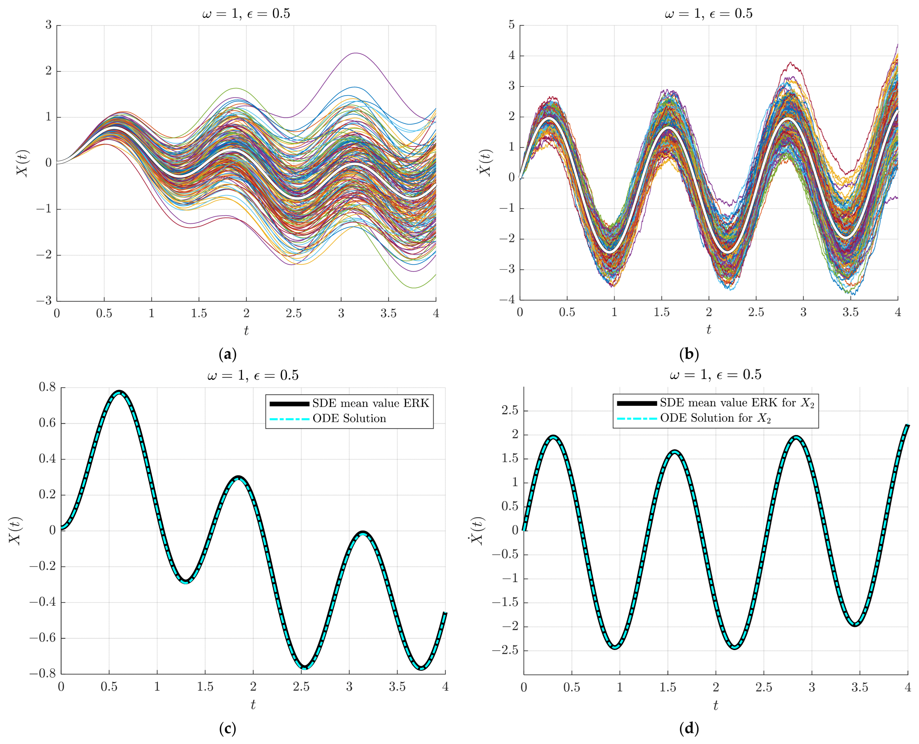
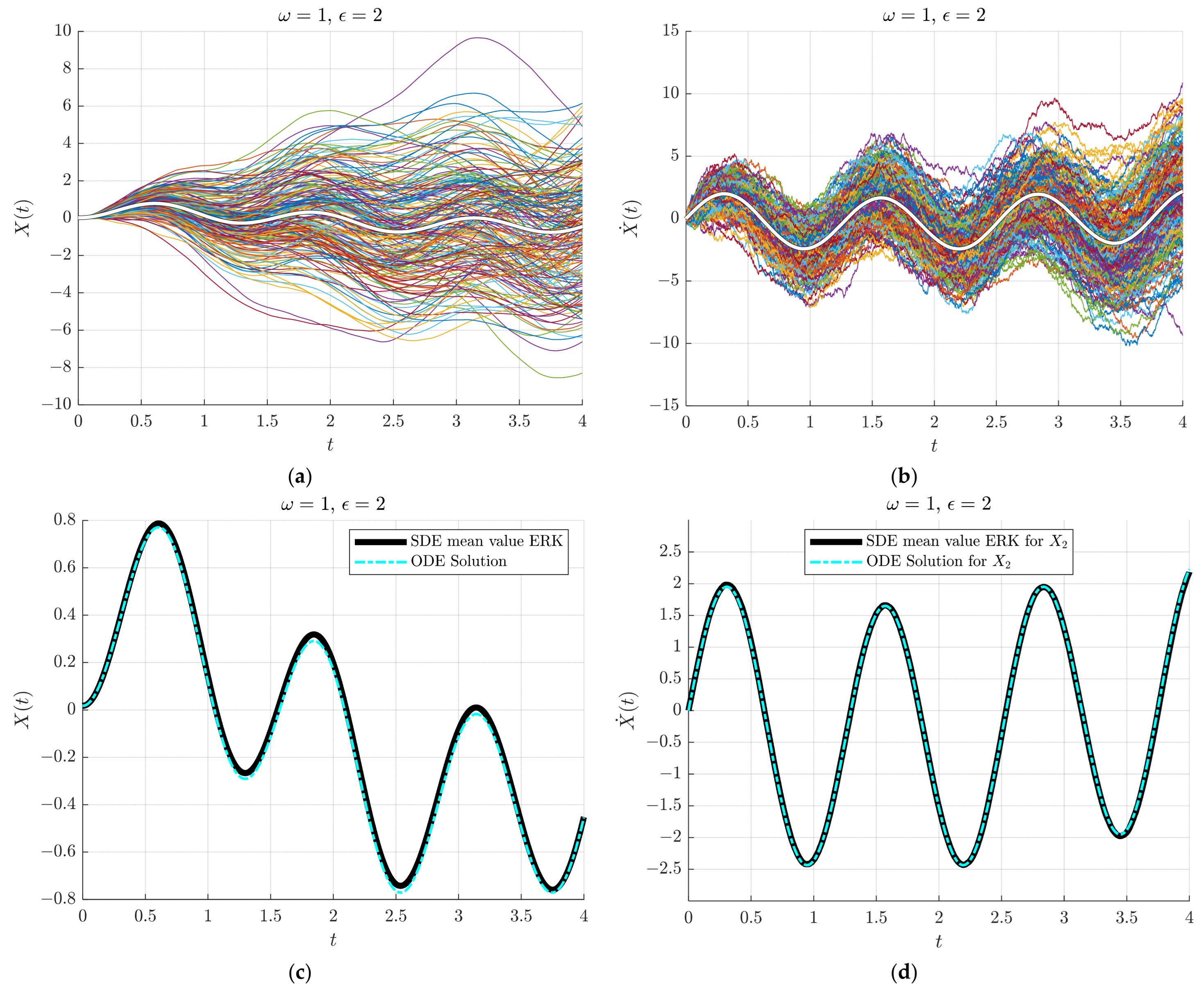
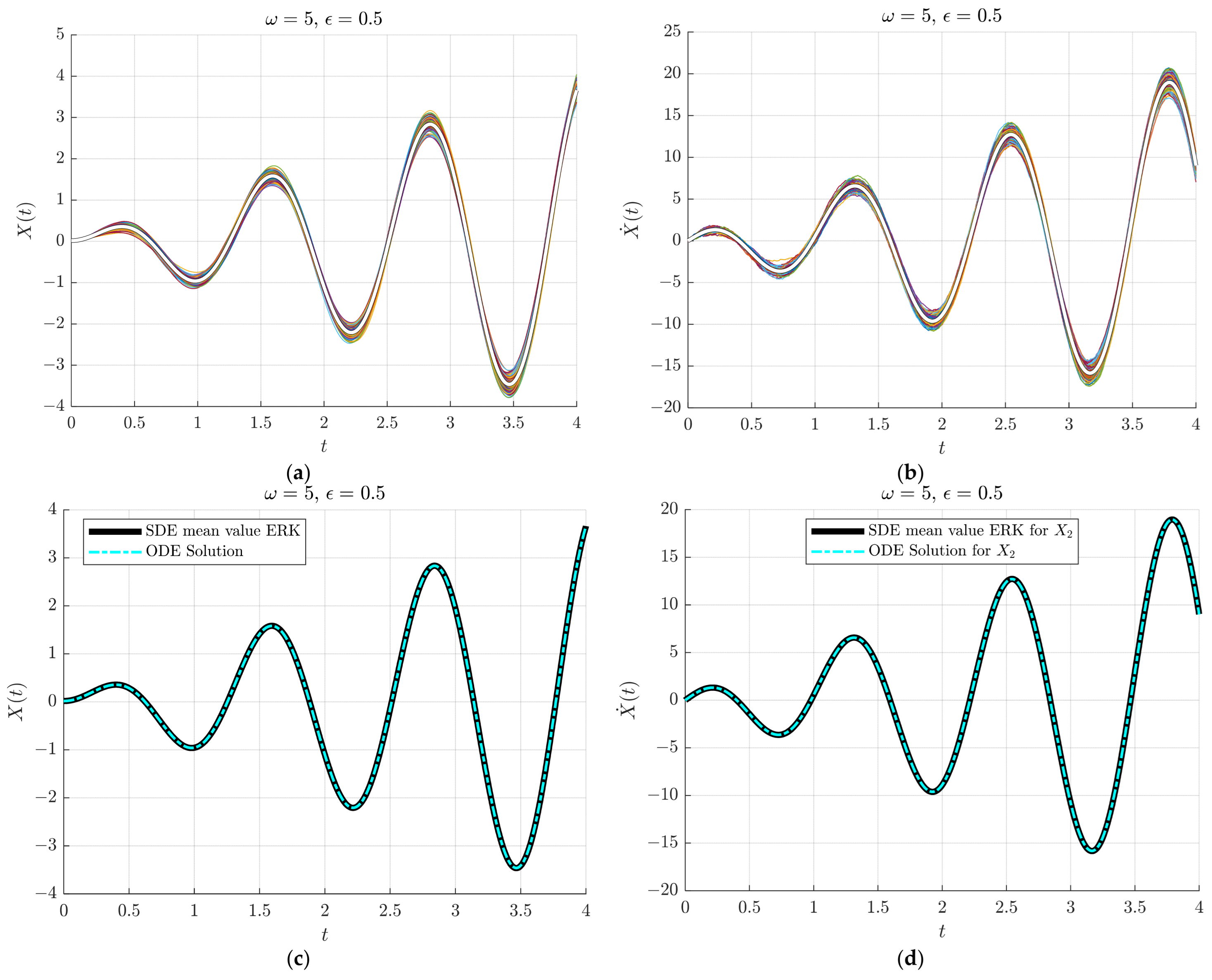
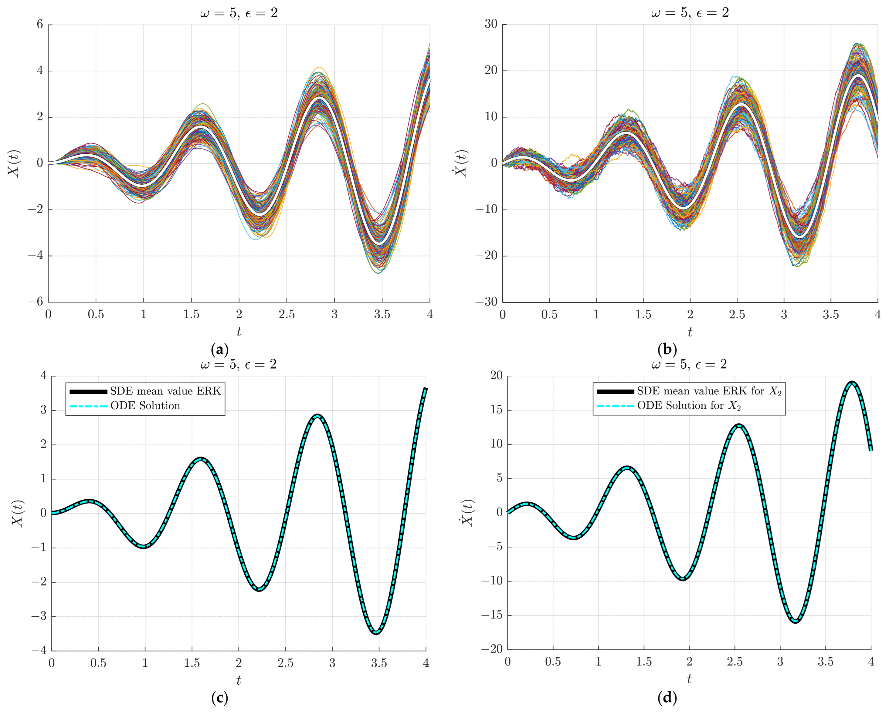
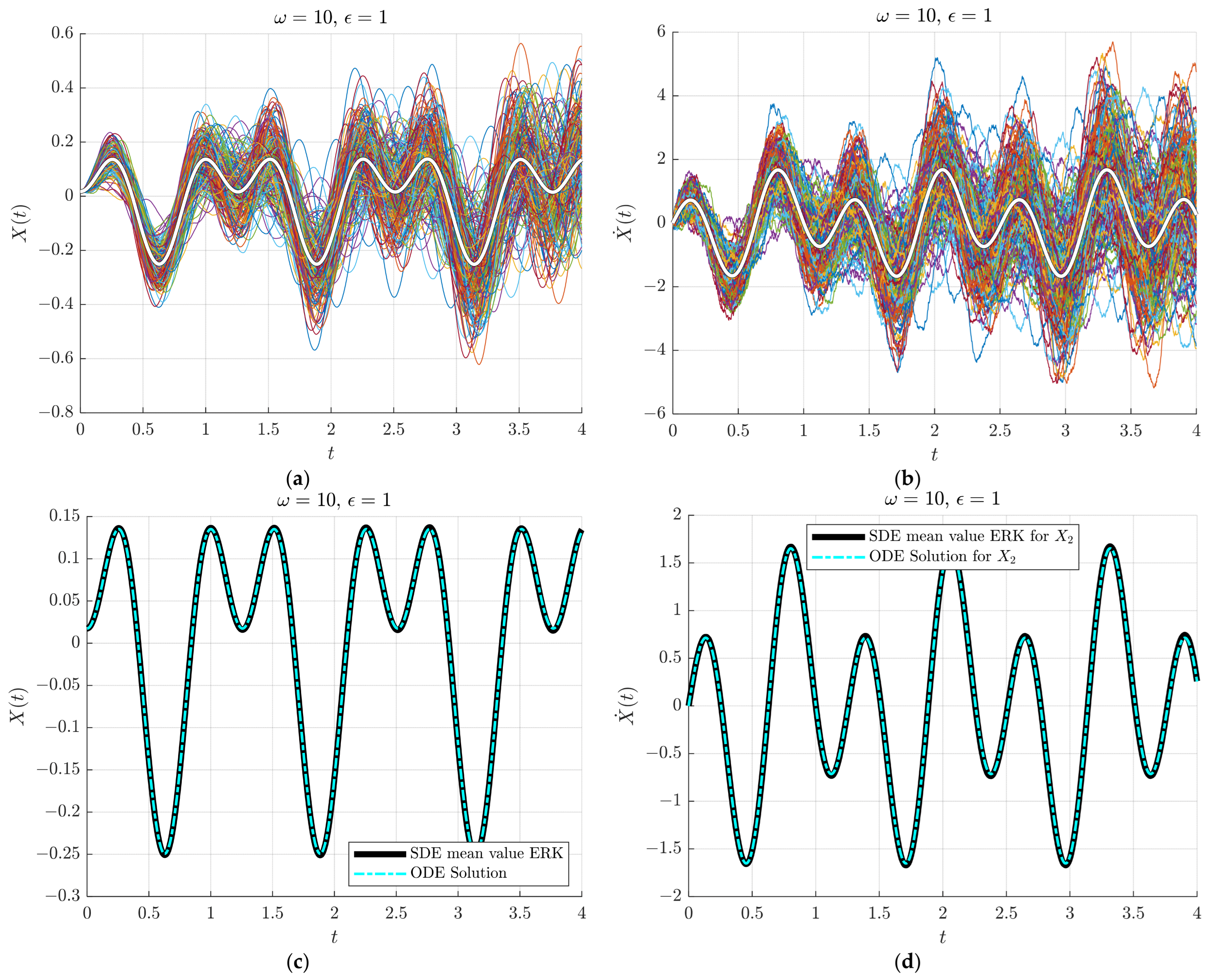
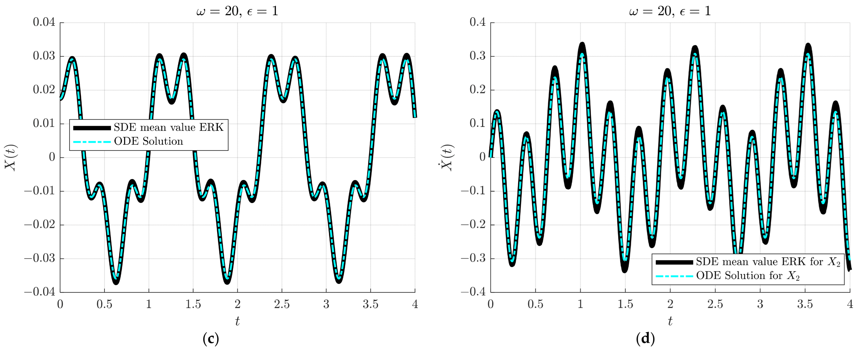
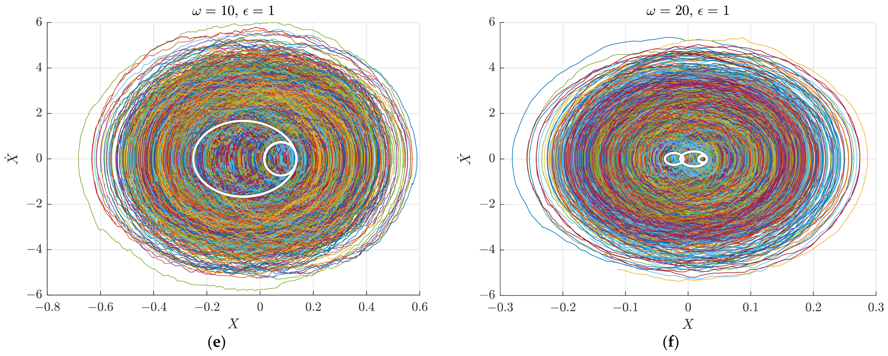
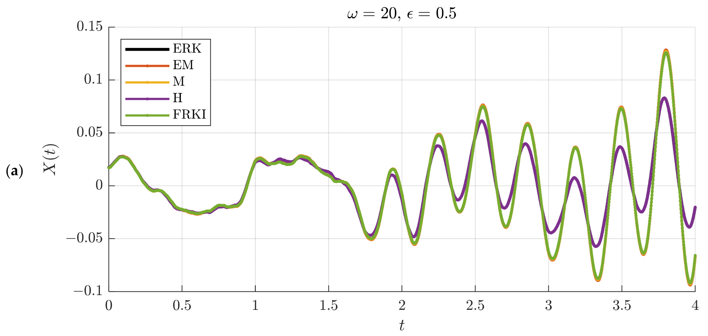
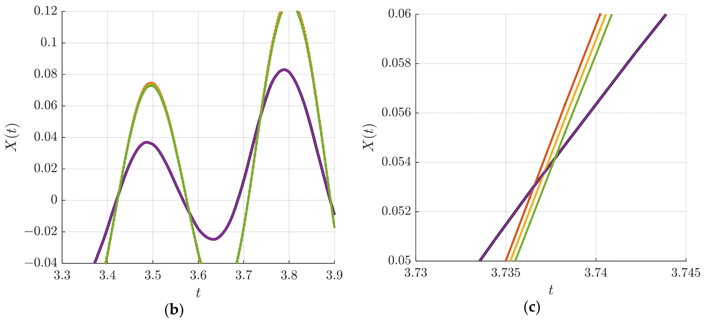
4.1. Test 1. The SDE of a Forced Undamped Oscillator with Exterior Stochastic Disturbance

Starting from the differential equation of the pitch angle of the satellite described previously, considering the simplified case for b = c = 0 and for small pitch angles, and adding a free term with an oscillating function h(t) and a stochastic term described by the constant ε to the equation, the following equation is obtained:

$$\ddot{x}+{\omega }^{2}x=\mathrm{h}\left(t\right)+\epsilon {\displaystyle \frac{\mathrm{dW}}{\mathrm{dt}}},x\left(0\right)={\displaystyle \frac{\pi }{180}},\dot{x}\left(0\right)=0,$$

(31)

in which $\mathrm{h}\left(t\right)={\mathrm{F}}_0\cos \left({\mathrm{\omega }}_{1}t\right)$, ${\mathrm{\omega }}^2=1-2{\mathrm{A}}_0$, and $\epsilon \in \mathbb{R}$. This equation was previously studied by the authors [22], without comparing the behaviour of the numerical schemes applied to this equation. This second-order stochastic differential equation of a forced undamped oscillator with exterior stochastic disturbance can be written as a two-dimensional system of first-order stochastic equation:

$$\mathrm{d}\mathbf{X}\left(t\right)=\mathrm{d}\left(\begin{array}{c}{\mathrm{X}}_1\left(t\right)\\ {\mathrm{X}}_2\left(t\right)\end{array}\right)=\left(\begin{array}{c}{\mathrm{X}}_2\left(t\right)\\ -{\mathrm{\omega }}^2{\mathrm{X}}_1\left(t\right)+\mathrm{h}\left(t\right)\end{array}\right)\mathrm{dt}+\left(\begin{array}{c}0\\ \epsilon \end{array}\right)\mathrm{dW}\left(t\right).$$

(32)

In the absence of an analytical solution for the stochastic differential system, the finite difference schemes can be compared, in the mean value, to the analytical solution of the “normal” differential equation (for ε = 0):

$$\ddot{x}\left(t\right)+{\mathrm{\omega }}^{2}x\left(t\right)={\mathrm{F}}_0\cos \left({\mathrm{\omega }}_{1}t\right),$$

(33)

for which two cases can be distinguished:

A.

Non-resonant case $\mathrm{\omega }\ne {\mathrm{\omega }}_1$.

In this case, the general solution determined by the summation of the homogenous and particular solutions [26,27,28] is as follows:

$$x\left(t\right)=\left(x\left(0\right)-{\displaystyle \frac{{\mathrm{F}}_0}{{\mathrm{\omega }}^2-{\mathrm{\omega }}_1^2}}\right)\cos \left(\mathrm{\omega }t\right)+{\displaystyle \frac{{\mathrm{F}}_0}{{\mathrm{\omega }}^2-{\mathrm{\omega }}_1^2}}\cos \left({\mathrm{\omega }}_{1}t\right).$$

(34)

B.

Resonant case $\mathrm{\omega }={\mathrm{\omega }}_1$.

For this case, the solution is as follows:

$$x\left(t\right)=x\left(0\right) \cos \left(\mathrm{\omega }t\right)+t{\displaystyle \frac{{\mathrm{F}}_0}{2{\mathrm{\omega }}_1}}\sin \left({\mathrm{\omega }}_{1}t\right).$$

(35)

The angular frequency of the perturbations and the amplitude for all the considered cases are ${{\mathrm{\omega }}_1=5,\mathrm{F}}_0=10$. The values of ε and ω were varied in order to see the impact of both white noise and the angular frequency of the stochastic pendulum on the results. The timestep considered for all of the following simulations results is Δt = 0.02, and the number of random paths considered is M = 5000. The time interval of integration is between t⁰ = 0 and T = 4 for the simulations. The relation between the timestep size, integration time, and number of calculation points (N_p) on a uniform grid is as follows:

$$\Delta \mathrm{t}={\displaystyle \frac{\mathrm{T}}{{\mathrm{N}}_{\mathrm{p}}-1}}.$$

(36)

The mean value of all of the 5000 trajectories of the SDE results obtained with the Efficient Runge–Kutta (ERK) method is compared with the result of the ODE in order to highlight the zero-mean property of the white noise and to prove the mean stability of the ERK method compared to the other schemes—Euler–Maruyama (EM), Milshtein (M), Stochastic Heun (H), and First order Runge–Kutta involving the Itô coefficient (FRKI).

In the following test, we want to study the impact of the SDE coefficients on the pitch angle and pitch angular velocity.

A1. This case is for an angular frequency ω = 1 and a small coefficient for the white noise ε = 0.5. Results can be seen in Figure 2.

Figure 2a shows the small disturbing effect of the white noise on both X and dX/dt. In the case of dX/dt (Figure 2b), the white noise has a more visible effect on the trajectories, causing them to look similar to a Wiener process, but maintaining the trend of the mean value (white trendline).

A2. This case is for an angular frequency ω = 1 and a larger coefficient for the white noise ε = 2. Results can be seen in Figure 3.

The growth of the white noise coefficient ε is followed by the growth in amplitude of the trajectories (see the y-axis scale of Figure 3 compared to the scale of the y-axis in Figure 2); there are also trajectories for which X appears to maintain a constant value for short time intervals. However, just like in the previous case, the mean value of the SDE trajectories obtained with the ERK scheme follows the ODE solution closely.

B1. This case is for a resonant angular frequency ω = ω₁ = 5 and a small coefficient for the white noise ε = 0.5. Results can be seen in Figure 4.

For the resonant case, the impact of the white noise is not as visible, as in the previous case, Figure 4. The growth in amplitude caused by the equality between the angular frequency of the stochastic oscillator and the angular frequency of the exterior stochastic perturbing force, which shadows the impact of the white noise. However, in the case of a smaller stochastic coefficient, it can be seen that the 5000 paths are more evenly distributed around the mean path, suggesting the symmetry of the zero-mean Gaussian white noise.

B2. This case is for a resonant angular frequency ω = ω₁ = 5 and a larger coefficient for the white noise ε = 2. Results can be seen in Figure 5.

The smoothness of any of the stochastic trajectories of X function of time, compared to the stochastic trajectories of dX/dt function of time—which look similarly to the Wiener process, with “rough” edges in the curves—is due to the fact that integrating a derivative function (dX/dt) over time is averaging that function (X). Furthermore, in the stochastic differential equation, the white noise only affects the equation of dX/dt, and not that of X itself.

In both of the resonance cases, the mean value of the ERK results follows the ODE solution precisely (Figure 4 and Figure 5).

A3. This case is for an angular frequency ω = 10 and a coefficient for the white noise ε = 2. Results can be seen in Figure 6.

A4. This case is for an angular frequency ω = 20 and a coefficient for the white noise ε = 1. Results can be seen in Figure 7.

All of the results for the different values of the constants are compared in the phase plane in the next figure, Figure 8.

Due to the properties of the Wiener process (normally distributed variable with zero-mean), in the resonant case, the stochastic trajectories are symmetrically distributed around the values of the ODE deterministic solution. The resonant evolution for the stochastic dynamical system can be plotted in a 3D graph (Figure 9).

Considering the fact that the local minima and maxima of the SDE trajectories do not occur at the same locations as the corresponding extrema of the ODE, the roots of the derivative function have different locations for different paths. Thus, another level of symmetry is displayed by the SDE considered: the symmetry of the SDE instantaneous states in the phase plane.

In order to compare the stability of the scheme, a comparison between the mean values of the schemes and ODE solution (Figure 10) and a comparison between each schemes for a random path (Figure 11) are presented below.

It is obvious that, in the mean value, the schemes EM, M, and FRKI display an instability, which is seen in the deviation from the ODE solution (Figure 10). The best performing schemes are Stochastic Heun (H) and Efficient Runge–Kutta (ERK). The locations of the maxima and minima of the mean value of the function X are, however, predicted correctly by all of the schemes, even if their values are not.

In terms of stability in the weak sense (convergence of random trajectories), in the absence of an analytical solution, one can observe, in Figure 11, a similar result as before. The two best performing (H and ERK) schemes maintain a stable trendline, while the other three schemes display the same instability towards the final timestep. The amplitude displayed by the “unstable” schemes has a more rapid growth than the H and ERK schemes. The roots of X and the locations of the maxima and minima are also different between the two categories of schemes: stable and unstable.

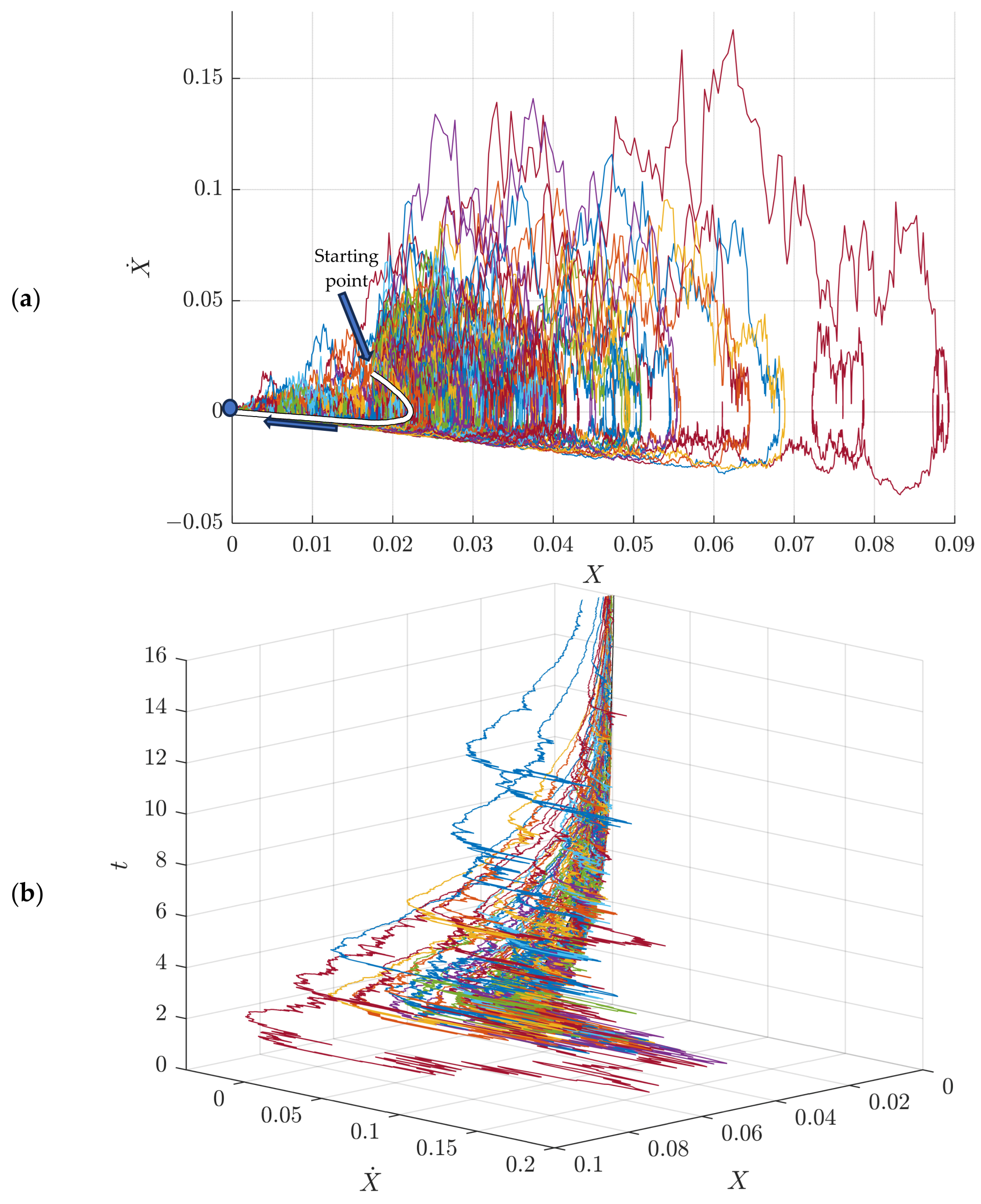
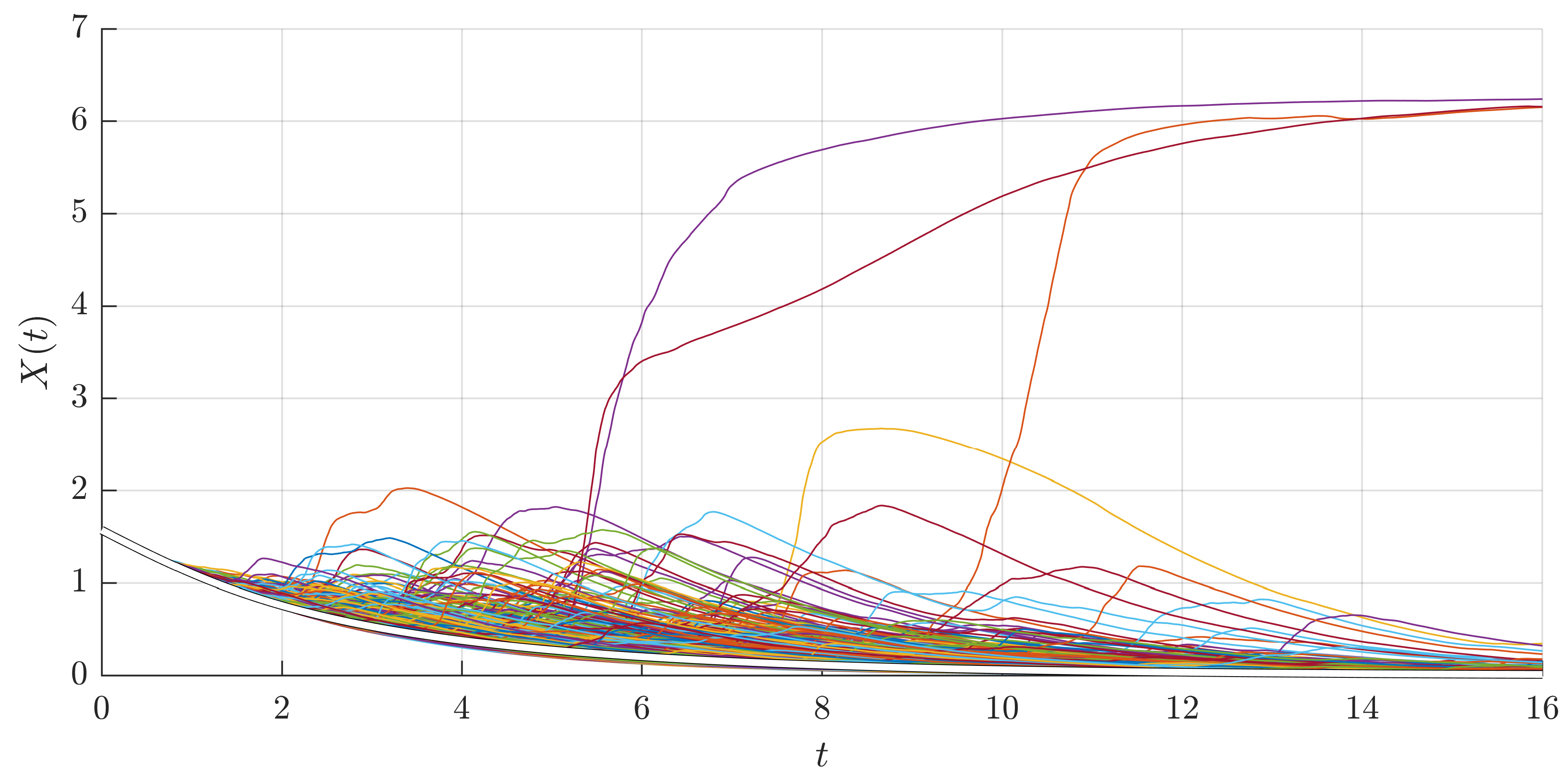
4.2. The Dimensionless SDE of the Pitch Angle of the Satellite

The stability condition for the SDE without the white noise (deterministic stability) is determined by calculating the eigenvalues of the Jacobian matrix of the ODE around the critical points (the roots of the linearized system $\dot{\mathbf{X}}=\mathrm{JX}$). These points are as follows:

$$\left(\mathrm{X},\dot{\mathrm{X}}\right)=\left\{\left(\mathrm{k}\pi ,0\right)\cup \left(\pm \arccos {\displaystyle \frac{1}{2{\mathrm{A}}_0}}+2\mathrm{k}\pi ,0\right)\right\},\mathrm{k}\in \mathrm{Z}.$$

(37)

Out of these roots, the origin (0,0) is the most relevant in this case. To find the eigenvalues, we solve

$$\det \left(\mathbf{J}-\lambda {\mathrm{I}}_3\right)=0,$$

(38)

in which the Jacobian matrix is evaluated at the origin:

$$\mathbf{J}={\left.\left(\begin{array}{cc}0& 1\\ -\cos \left({\mathrm{X}}_1\right)+2{\mathrm{A}}_0\cos \left(2{\mathrm{X}}_1\right)& -\mathrm{b}\end{array}\right)\right|}_{\left({\mathrm{X}}_1,{\mathrm{X}}_2\right)=\left(0,0\right)}=\left(\begin{array}{cc}0& 1\\ 2{\mathrm{A}}_0-1& -\mathrm{b}\end{array}\right).$$

(39)

The characteristic equation is given by the following:

$${\lambda }^2+\lambda \mathrm{b}-\left(2{\mathrm{A}}_0-1\right)=0,$$

(40)

and the corresponding roots are as follows:

$${\lambda }_{\mathrm{1,2}}={\displaystyle \frac{-\mathrm{b}\pm \sqrt{{\mathrm{b}}^2+4\left(2{\mathrm{A}}_0-1\right)}}{2}}.$$

(41)

According to the Stability Criteria for Linearization of 2D Systems stability criterion [29], the critical point of an ODE is an attractor if and only if the eigenvalues of the linearised matrix J have negative real parts. As b is a real positive number, this leads to negative real eigenvalues with the following condition:

$${\mathrm{A}}_0<{\displaystyle \frac{1}{2}}, \forall b\in {\mathbb{R}}_{+},$$

(42)

and to complex eigenvalues with negative real parts:

$${\mathrm{A}}_0<{\displaystyle \frac{4-{\mathrm{b}}^2}{8}}.$$

(43)

The stochastic stability of SDEs was previously studied, theorised, and formulated in various publications [30,31], and the stochastic stability of the pitch angle equation of motion was studied by Sagirow [1], and the relationship between the constants of the SDE which dictates the stability of the equation is the following:

$${\mathrm{A}}_0\le {\displaystyle \frac{1}{2}}\left(1-{\displaystyle \frac{{\mathrm{c}}^2}{2\mathrm{b}-{\mathrm{c}}^2{\mathrm{b}}^2}}\right).$$

(44)

We remark that, for c = 0, we re-obtain the same condition as discussed previously for the deterministic case.

4.2.1. Case 1

The proposed initial conditions are as follows:

$${\mathrm{X}}_0={\dot{\mathrm{X}}}_0=\pi /180,$$

(45)

which are very close from the stability point (0.0). Taking into consideration the previous conditions for stability, the constants considered for this SDE are as follows:

$${\mathrm{A}}_0=0.25, \mathrm{b}=2, \mathrm{c}=0.8.$$

(46)

The graphical results of this SDE are shown in the following figures.

In Figure 12, we represent the phase plane and the evolution in the dimensionless time of the 5000 trajectories. As was previously demonstrated, the pitch angle motion stabilises (or is asymptotically stable [26]) at the origin (0,0) after a short interval of time for all paths. A comparison between the results obtained with the schemes can be seen below in Figure 13.

4.2.2. Case 2

In order to test the other stability points, we can consider the next initial values:

$${\mathrm{X}}_0=\pi /2, {\dot{\mathrm{X}}}_0=-1/2,$$

(47)

for which the results can be seen below.

One can notice that, in Figure 14, although most of the trajectories stabilise at the origin, which is the globally equilibrium point, some of these 5000 cases stabilise at $\mathrm{X}=2\pi$. We are referring to the white noise that has a decisive effect on the stability of the dynamical system.

4.2.3. Case 3

Let us consider another set of initial values:

$${\mathrm{X}}_0=\pi /2, {\dot{\mathrm{X}}}_0=1/2,$$

(48)

for which we obtain the results in Figure 15.

Although the noiseless differential equation will stabilise at the origin, there are certain paths for which stabilisation occurs at different points (for X = 2kπ), highlighting the uncertainty associated with SDEs and the importance of stability conditions.

It is obvious that, for the deterministic case (c = 0), for any initial condition, the trajectory evolution of the system will be stabilised on the closest point of equilibrium, which takes the form of (2kπ,0). One must remark that, although the initials are the same for all of the 5000 paths, there are three distinct points at which groups of these paths are asymptotically stable: (0,0), (2π,0), and (4π,0). In other words, if the system is asymptotically stable, in the present example, stability is achieved on any of the paths, but one cannot anticipate precisely on which of the equilibrium points each path will stabilise, nor can one tell the number of paths which will stabilise at a certain point.

4.2.4. Case 4

Let us consider another set of initial values:

$${\mathrm{X}}_0=20, {\dot{\mathrm{X}}}_0=20.$$

(49)

This last case was considered to show that, depending on the initial conditions for the SDE system, the number of equilibrium points are increased as long as the point ${(\mathrm{X}}_0, {\dot{\mathrm{X}}}_0)$ is farther from the origin of the phase plane. Each of the trajectories is asymptotically stable (as time goes to infinity), as we can see in Figure 16, to numerous equilibrium points, which are multiples of 2π. The number of equilibrium points remains, for the moment, unclear, as we did not find any correlation between the position of the starting point and the points of the type (2kπ,0). In this case, $k\le 41$.

The stabilisation of the stochastic paths in the numerous equilibrium points resembles the first level in a fractal tree. Considering the possibility of another external disturbance occurring on the satellite (such as a collision with a small object) having an effect on the system much like the initial values of the stochastic pitch angle, each of the previous equilibrium points of the system would generate another set of stabilisation points after the disturbance, thus creating another layer in this fractal tree.

5. Conclusions

This work aimed to analyse the stability of a satellite’s orbit around the Earth in the case of a stochastic atmosphere density. Starting from the equations of motion (the equations of the angular momentum of a rigid) and applying simplifying assumptions, a nonlinear, non-homogenous, second-order stochastic differential equation (SDE) was derived.

To support this analysis, elements of probability theory, mathematical statistics, and stochastic calculus were briefly introduced. Five finite difference schemes used in solving the second-order stochastic differential equation were analysed and tested for differences. In total, 5000 random trajectories were considered, from which a path was randomly chosen, for which the results of the schemes were superimposed to estimate their accuracy and stability. From all of the schemes, the ERK (i.e., Efficient Runge–Kutta) gives the best results. The simplified case of the satellite stochastic system was studied starting from the differential equation of the pitch angle obtained from the analysis of the stability of the orbit of a satellite, a second-order system of stochastic differential equations. The stability of the ODE (without white noise) was studied and compared to the stability of the SDE. The behaviour of the stochastic dynamic system was analysed, and stabilisation was confirmed by the results.

The pitch angle stability SDE system is similar to the system one obtained in the case of an undamped forced oscillator with external stochastic disturbance. The analytical solution for the deterministic differential equation (in the absence of white noise) was compared to the average of the 5000 random trajectories. The conclusion reached from this comparison confirmed the convergence in the mean to the solution of the deterministic equation and the zero-mean property of the Wiener process, regardless of ε (the coefficient by which the stochastic noise is multiplied). However, if, in the case of the ideal oscillator with forced movements without a stochastic component, the oscillator is stable for any proper pulsation different from that of the forced movements, oscillating around the equilibrium position, in the case of stochastic (or “noisy”) forced movements, the amplitude of the oscillations is amplified over time, no longer being able to reach stability.

The examples studied and the results obtained in this paper are a first step taken in a very important research direction—the study of the stability of the stochastic orbit of a satellite and, implicitly, also stochastic numerical methods, which, although being a field researched in the international literature, is still subject to scientific debate. The authors believe that there is a need for a greater deepening of theoretical knowledge in stochastic computing, and especially on stochastic systems with larger dimensions and more types of noise (i.e., vector Wiener processes). In the future, the authors intend to analyse physical phenomena that are reduced to stochastic systems with multidimensional noise, implementing other schemes with finite differences in the high-convergence-order Runge–Kutta type in solving them.

As a general conclusion, we can affirm that, if the stability condition is met, the stochastic pitch angle system will stabilise on any of the (2kπ,0) points. Basically, being complete rotations, the satellite is brought to the equilibrium position (attitude).The solution paths of a stochastic differential equation (SDE) can be understood as the trajectories of a dynamical system influenced by stochastic processes. Visualising these trajectories can be achieved by plotting the numerical approximations of multiple sample paths. These visualisations offer a possibility to interpret the behaviour and the dynamics of a stochastic system.

References

1. Sagirow, P. (Ed.) Stochastic Dynamical Systems. In Stochastic Methods in the Dynamics of Satellites: Course Held at the Department for General Mechanics; Springer: Vienna, Austria, 1970; pp. 8–47. [Google Scholar] [CrossRef]
2. Beletskii, V.V. Motion of an Artificial Satellite About Its Center of Mass. In Mechanics of Space Flight; Israel Program for Scientific Translation: Jerusalem, Israel, 1966. [Google Scholar]
3. Toral, R.; Colet, P. Introduction to Stochastic Processes. In Stochastic Numerical Methods; John Wiley & Sons, Ltd.: Hoboken, NJ, USA, 2014; pp. 167–190. [Google Scholar] [CrossRef]
4. Evans, L.C. An Introduction to Stochastic Differential Equations; American Mathematical Society: Providence, RI, USA, 2012; ISBN 1470410540. [Google Scholar]
5. Itô, K. Stochastic integral. Proc. Jpn. Acad. Ser. Math. Sci. 1944, 20, 519–524. [Google Scholar] [CrossRef]
6. Capasso, V.; Bakstein, D. An introduction to continuous-time stochastic processes: Theory, models, and applications to finance, biology, and medicine. In Modeling and Simulation in Science, Engineering and Technology; Birkhäuser: Boston, MA, USA; Basel, Switzerland; Berlin, Germany, 2005. [Google Scholar]
7. Dupačová, J.; Hurt, J.; Štěpán, J. Stochastic modeling in economics and finance. In Applied Optimization; No. 75; Kluwer Academic Publishers: Dordrecht, The Netherlands; Boston, MA, USA; New York, NY, USA; London, UK; Moscow, Russia, 2002. [Google Scholar]
8. Andersson, H.; Britton, T. Stochastic epidemic models and their statistical analysis. In Lecture Notes in Statistics; No. 151; Springer: New York, NY, USA; Berlin/Heidelberg, Germany, 2000. [Google Scholar]
9. Voinea, R.; Stroe, I.V.; Predoi, M.V. Technical Mechanics; Politehnica Press: Bucureşti, Romania, 2010. [Google Scholar]
10. Rao, A.V. Dynamics of Particles and Rigid Bodies: A Systematic Approach; Cambridge University Press: Cambridge, UK; New York, NY, USA, 2006. [Google Scholar]
11. Bogoi, A.; Dănăilă, S.; Isvoranu, D. Ecuații Generale de Transport ale Dinamicii Fluidelor; Monitorul Official: București, Romania, 2021. [Google Scholar]
12. Gillies, G.T. The Newtonian gravitational constant: Recent measurements and related studies. Rep. Prog. Phys. 1997, 60, 151–225. [Google Scholar] [CrossRef]
13. Li, Q.; Xue, C.; Liu, J.-P.; Wu, J.-F.; Yang, S.-Q.; Shao, C.-G.; Quan, L.-D.; Tan, W.-H.; Tu, L.-C.; Liu, Q.; et al. Measurements of the gravitational constant using two independent methods. Nature 2018, 560, 582–588. [Google Scholar] [CrossRef] [PubMed]
14. Goldstein, H. Classical Mechanics, 2nd ed.; Addison-Wesley Series in Physics; Addison-Wesley: Reading, MA, USA; Menlo Park, CA, USA; London, UK, 1981. [Google Scholar]
15. Schrello, D.M. Dynamic Stability of Aerodynamically Responsive Satellites. J. Aerosp. Sci. 1962, 29, 1145–1155. [Google Scholar] [CrossRef]
16. Sheporaitis, L.P. Stochastic stability of a satellite influenced by aerodynamic and gravity gradient torques. AIAA J. 1971, 9, 218–222. [Google Scholar] [CrossRef]
17. Mostaza-Prieto, D. Characterisation and Applications of Aerodynamic Torques on Satellites. Ph.D. Thesis, The University of Manchester, Manchester, UK, 2017. [Google Scholar]
18. Kutiev, I.; Tsagouri, I.; Perrone, L.; Pancheva, D.; Mukhtarov, P.; Mikhailov, A.; Lastovicka, J.; Jakowski, N.; Buresova, D.; Blanch, E.; et al. Solar activity impact on the Earth’s upper atmosphere. J. Space Weather Space Clim. 2013, 3, A06. [Google Scholar] [CrossRef]
19. Kloeden, P.E.; Platen, E. Numerical Solution of Stochastic Differential Equations; Springer: Berlin/Heidelberg, Germany, 1992. [Google Scholar] [CrossRef]
20. Durrett, R. Probability: Theory and Examples, 5th ed.; Cambridge University Press: Cambridge, UK, 2019. [Google Scholar]
21. Mörters, P.; Peres, Y.; Schramm, O.; Werner, W. Brownian motion. In Cambridge Series in Statistical and Probabilistic Mathematics; No. 30; Cambridge University Press: Cambridge, UK, 2010. [Google Scholar]
22. Bogoi, A.; Dan, C.-I.; Strătilă, S.; Cican, G.; Crunteanu, D.-E. Assessment of Stochastic Numerical Schemes for Stochastic Differential Equations with “White Noise” Using Ito’s Integral’. Symmetry 2023, 15, 2038. [Google Scholar] [CrossRef]
23. Saito, Y.; Mitsui, T. Stability Analysis of Numerical Schemes for Stochastic Differential Equations. SIAM J. Numer. Anal. 1996, 33, 2254–2267. [Google Scholar] [CrossRef]
24. Milʹshteĭn, G.N. Numerical Integration of Stochastic Differential Equations; Springer: Dordrecht, The Netherlands, 2011. [Google Scholar]
25. Saito, Y.; Mitsui, T. Discrete approximations for stochastic differential equations. Trans. Jpn. SIAM 1992, 746, 1–16. [Google Scholar]
26. Bogoi, A.; Cican, G.; Daniel-Eugeniu, C. Fundamentals of Acoustics; Lecture Notes for Engineers; Editura Monitorul Official: Bucureşti, Romania, 2024. [Google Scholar]
27. Bacalu, I.; Şerbănescu, C. Ecuaţii Diferenţiale: Culegere de Probleme: Compendiu; Printech: Bucureşti, Romania, 2013. [Google Scholar]
28. Boyce, W.E.; DiPrima, R.C. Elementary Differential Equations and Boundary Value Problems, 8th ed.; Wiley: Hoboken, NJ, USA, 2005. [Google Scholar]
29. Leipholz, H. Stability Theory, 2nd ed.; Vieweg+Teubner Verlag: Weisbaden, Germany, 1987. [Google Scholar]
30. Tunç, O.; Tunç, C. On the asymptotic stability of solutions of stochastic differential delay equations of second order. J. Taibah Univ. Sci. 2019, 13, 875–882. [Google Scholar] [CrossRef]
31. Zouine, A.; Imzegouan, C.; Bouzahir, H.; Tunç, C. General decay stability of nonlinear delayed hybrid stochastic system with switched noises. Appl. Set-Valued Anal. Optim. 2024, 6, 157–177. [Google Scholar] [CrossRef]
Figure 1. The Euler angles of the satellite and the angular speed vectors—the pitch angular velocity (red), the yaw angular velocity (green), the roll angular velocity (blue) and the angular velocity of the satellite mass centre around the centre of The Earth (orange).
Symmetry 17 00402 g001
Figure 2. A1 test case (ω = 1, ε = 0.5), (a) mean value of X (white) and all trajectories (the coloured lines), (b) mean value of dX/dt (white) and all trajectories, and comparison between the ODE solution and the mean value of the ERK scheme for (c) X and (d) dX/dt.
Symmetry 17 00402 g002
Figure 3. A2 test case (ω = 1, ε = 2), (a) mean value of X (white) and all trajectories (the coloured lines), (b) mean value of dX/dt (white) and all trajectories, and comparison between the ODE solution and the mean value of the ERK scheme for (c) X and (d) dX/dt.
Symmetry 17 00402 g003
Figure 4. B1 resonant test case (ω = 5, ε = 0.5), (a) mean value of X (white) and all trajectories (the coloured lines), (b) mean value of dX/dt (white) and all trajectories, and comparison between the ODE solution and the mean value of the ERK scheme for (c) X and (d) dX/dt.
Symmetry 17 00402 g004
Figure 5. B2 resonant test case (ω = 5, ε = 2), (a) mean value of X (white) and all trajectories (the coloured lines), (b) mean value of dX/dt (white) and all trajectories, and comparison between the ODE solution and the mean value of the ERK scheme for (c) X and (d) dX/dt.
Symmetry 17 00402 g005
Figure 6. A3 test case (ω = 10, ε = 1), (a) mean value of X (white) and all trajectories (the coloured lines), (b) mean value of dX/dt (white) and all trajectories, and comparison between the ODE solution and the mean value of the ERK scheme for (c) X and (d) dX/dt.
Symmetry 17 00402 g006
Figure 7. A4 test case (ω = 20, ε = 1), (a) mean value of X (white) and all trajectories (the coloured lines), (b) mean value of dX/dt (white) and all trajectories, and comparison between the ODE solution and the mean value of the ERK scheme for (c) X and (d) dX/dt.
Symmetry 17 00402 g007aSymmetry 17 00402 g007b
Figure 8. Result comparison for the ERK Scheme in the phase plane between the 5000 trajectories (the coloured lines) and the mean trajectory (white).
Symmetry 17 00402 g008aSymmetry 17 00402 g008b
Figure 9. Results of the SDE for the 5000 trajectories (the coloured lines) obtained using the ERK Scheme for its evolution in dimensionless time for ω = 5, ε = 0.5 (a) and ω = 5, ε = 2 (b).
Symmetry 17 00402 g009
Figure 10. (a) Comparison between the schemes in the mean value and the ODE solution, (b,c) zoomed regions (the legend is shown in (a)).
Symmetry 17 00402 g010
Figure 11. (a) Comparison between the schemes for a random path, (b,c) zoomed regions (the legend is shown in (a)).
Symmetry 17 00402 g011aSymmetry 17 00402 g011b
Figure 12. Results of the SDE for the 5000 trajectories (the coloured lines) and the mean value (white) obtained using the ERK Scheme for (a) the phase plane and (b) its evolution in dimensionless time.
Symmetry 17 00402 g012
Figure 13. Comparison between the five schemes for (a) the evolution of mean value in time (b) zoomed region and (c) a random path of the pitch angle (d) zoomed region.
Symmetry 17 00402 g013
Figure 14. Stability analysis displaying two different stabilisation tendencies for the 5000 trajectories (the coloured lines) and the mean value (white).
Symmetry 17 00402 g014
Figure 15. Stability analysis displaying two different stabilisation tendencies for the 5000 trajectories (the coloured lines) and the mean value (white).
Symmetry 17 00402 g015
Figure 16. Stability analysis displaying many different stabilisation tendencies for the 5000 trajectories (the coloured lines) and the mean value (white).
Symmetry 17 00402 g016