Joint Prediction of Li-Ion Battery Cycle Life and Knee Point Based on Early Charging Performance

Abstract

With the rapid development of lithium-ion batteries, predicting battery life is critical to the safe operation of devices such as electric ships, electric vehicles, and energy storage systems. Given the complexity of the internal aging mechanism of batteries, their aging process exhibits prominent nonlinear characteristics. Knee point, as a distinctive sign of this nonlinear aging process, plays a crucial role in predicting the battery’s lifetime. In this paper, the cycle life and cycle to the knee point of the battery are firstly predicted using the time dimension and space dimension features of the early external characteristics of the battery, respectively. Then, to capture the aging characteristics of batteries more comprehensively, we innovatively propose a joint prediction method of battery cycle life and knee point. Knee point features are incorporated into the battery cycle life prediction model in this method to fully account for the nonlinear aging characteristics of batteries. The experimental validation results show that the TECAN model, which combines time series features and knee point information, performs well, with a root mean square error (RMSE) of 106 cycles and a mean absolute percentage error (MAPE) of only 12%.

1. Introduction

With the increase of global environmental awareness and the transformation of energy structures, electric ships, as an important part of green shipping, are gradually becoming a new trend in the development of the shipping industry [1,2]. The research on modern hybrid energy ships covers various aspects, such as optimized scheduling [3] and battery power [4]. In this context, the performance and lifetime of lithium-ion batteries (LIBs), as the core energy storage devices of electric ships, are directly related to the range, operational efficiency, and safety of ships. Therefore, accurately predicting the life of new marine LIB energy storage systems is of great significance for optimizing battery management, improving battery usage efficiency, and ensuring safe ship operation [5].

Lithium-ion batteries have been widely used in many fields, such as electric vehicles, energy storage systems, and electric ships, due to their high energy density and long cycle life [6]. Taking electric ships as an example, with the prolongation of the battery usage time, its performance will gradually decay, and the battery will undergo a nonlinear aging process until it cannot meet the standard operation requirements of the ship. The nonlinear aging process is mainly reflected in the battery capacity decreasing slowly before the knee point and accelerating after the knee point [7]. The end-of-life (EOL) is reached when the remaining capacity is less than 80% of the nominal capacity. Therefore, early battery cycling characteristics and cycle to the knee (CTK) are utilized to predict cycle life (CL) to facilitate the timely detection of trends in battery performance. It provides a scientific basis for battery maintenance, replacement, and ship scheduling, thus avoiding the safety hazards and economic losses caused by battery failure.

Researchers have used various methods to predict the CL of Li-ion batteries effectively. Model-based techniques, such as electrochemical, thermal, and aging models, predict battery life by describing the battery’s reaction processes and aging rates [8,9]. However, these methods require precise battery parameters and complex computational processes. Another approach is based on data-driven prediction; methods such as recurrent neural networks (RNNs), long short-term memory (LSTM), multi-head attention mechanisms, and temporal convolutional networks (TCNs) have shown good predictive ability. RNN-based frameworks can predict capacity trajectories using only a small amount of historical data. However, the method suffers from the problem of forgetting early information when the time series is too long [10]. LSTM, as a time-series model that retains all the sequence information, is commonly used for battery capacity prediction [11,12]. However, it has limitations in regard to efficient feature extraction, especially when dealing with complex patterns and small datasets. Ge et al. employed a multi-head attention mechanism to predict battery life accurately [13]. 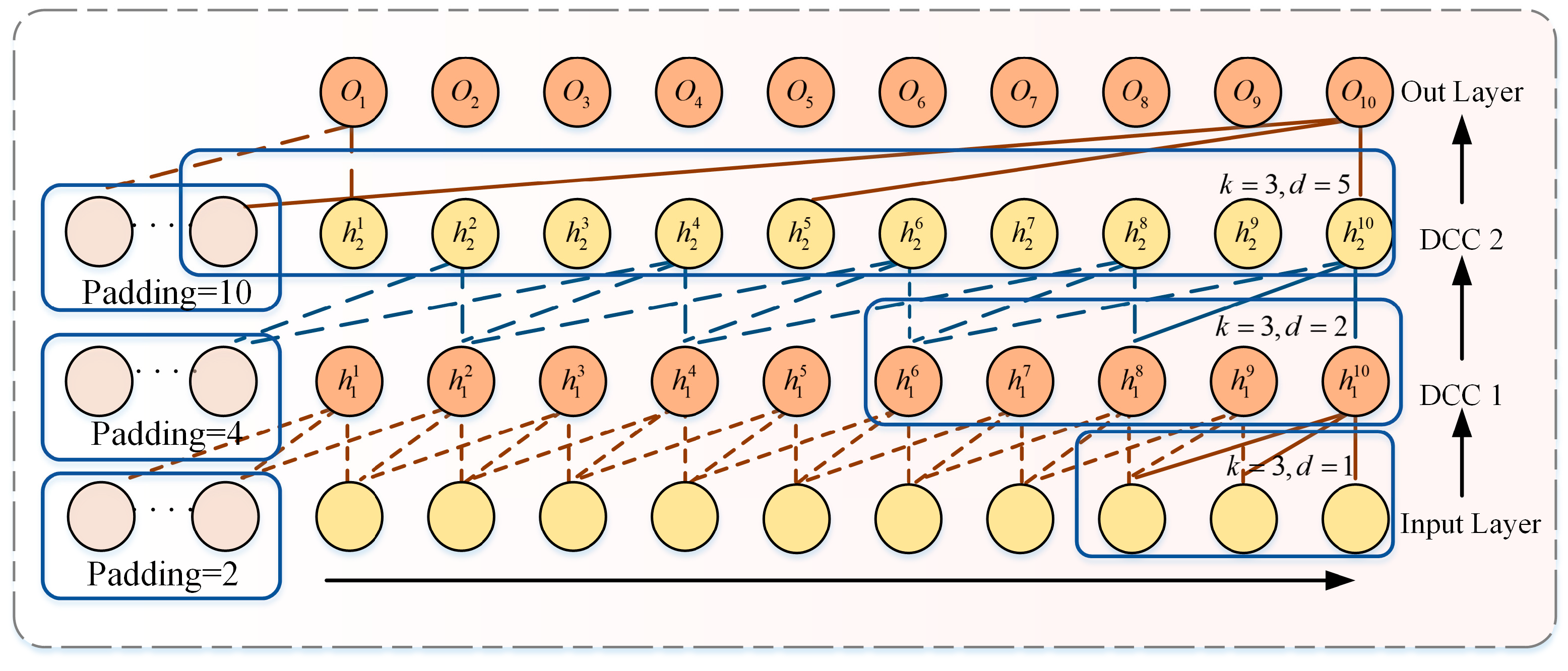This mechanism captures the complex relationships between different parts of the input data for efficient feature extraction. However, it is worth noting that a high computational cost accompanies the multi-head attention mechanism, while sufficient input data are usually required to ensure the prediction accuracy. On the other hand, TCNs are known for their parallel computing capabilities and efficient processing of long time-series data but may fail to highlight important features in deep structures [14]. 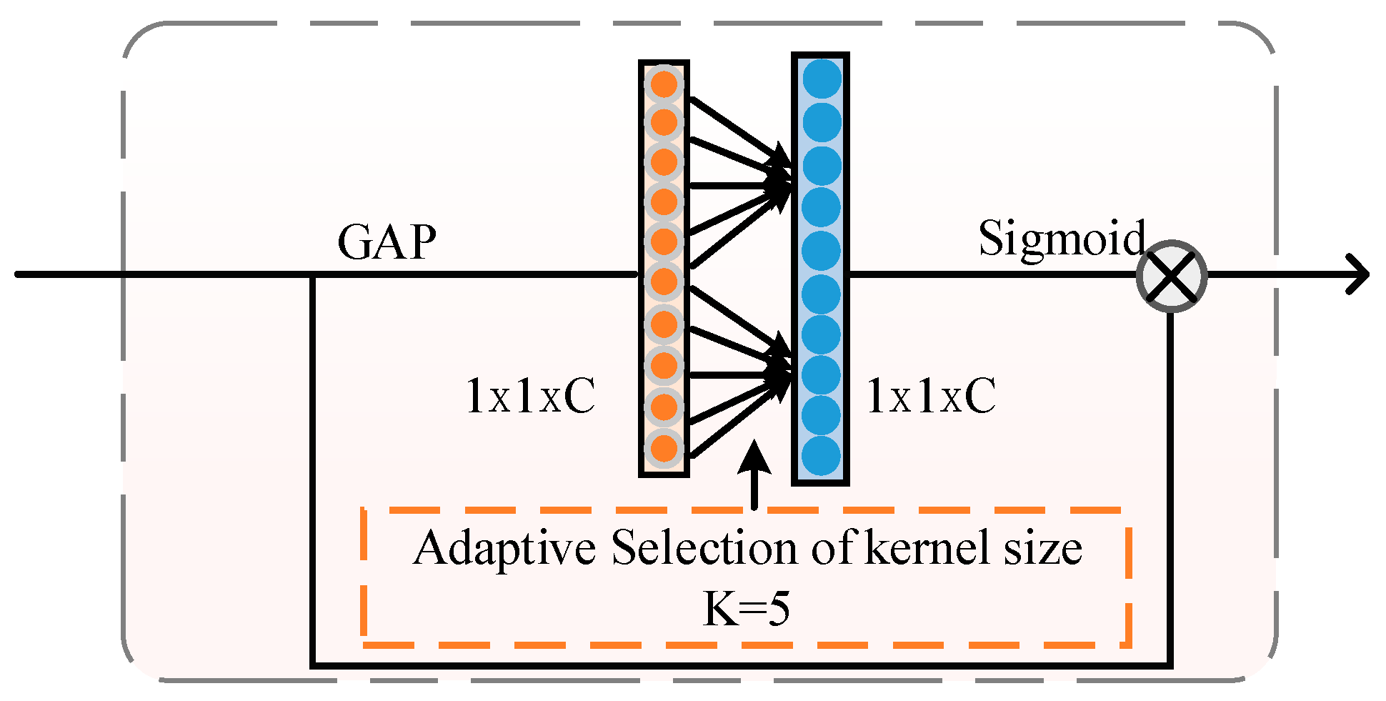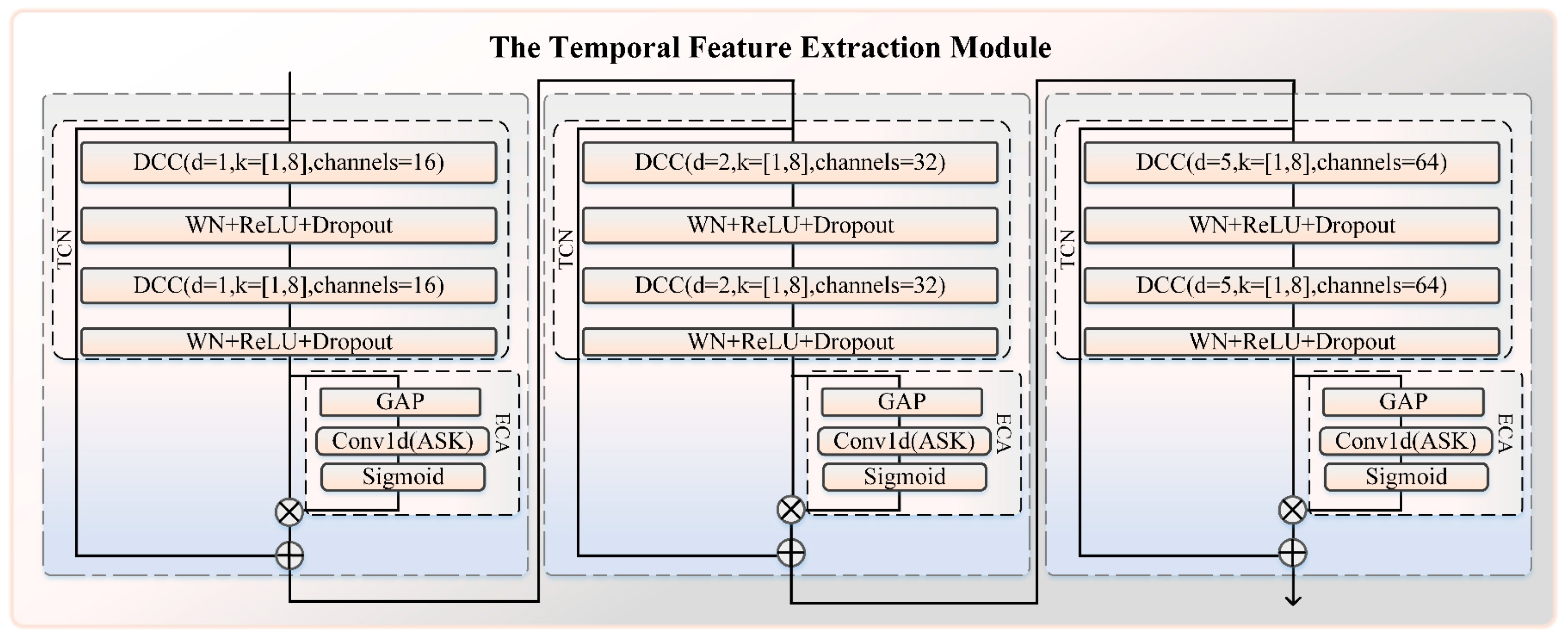Given this, this paper innovatively incorporates the efficient channel attention (ECA) mechanism into TCN, aiming to remedy this deficiency. ECA enhances TCN’s ability to capture key features, which not only optimizes the highlighting of information in focus but also improves the sensitivity and accuracy of the model in dealing with battery capacity prediction, especially in the face of multi-level feature interactions and nonlinear variations.

In addition, fusion models are also commonly used in battery life prediction to improve the accuracy and robustness of the prediction by integrating the advantages of different models. Xue and Chen used the combination of an adaptive untraceable Kalman filter (AUKF), support vector regression (SVR), a graphical neural network (GNN), and a particle filter (PF), respectively. However, the latter has the limitation of dynamic updating [15,16,17]. Li used the synergy of SVR and PF to optimize the bi-exponential model and enhance the accuracy of the capacity prediction [18]. Ma proposed combining the physical model with a deep neural network (DNN), emphasizing the accuracy of prediction and model interpretability [19]. Additionally, LSTM is often combined with other algorithms. Safitri et al. aimed to balance data simplification and feature preservation by optimizing the structure by combining gated recurrent units (GRU) with LSTM [20]. Further, scholars integrated LSTM with vibration modal decomposition (VMD) and Gaussian process regression (GPR) algorithms, first utilizing VMD to perform fine frequency splitting of the data and then LSTM, focusing on the prediction of the residual components, while GPR is responsible for the capacity regeneration part, in order to achieve accurate prediction of the capacity of lithium-ion batteries [21]. To address the challenges of insufficient feature extraction and the dependence of prediction accuracy on data strength, the study proposes a framework that combines a generalized learning system (BLS) with LSTM. The BLS is used for high-level feature extraction, and subsequently, LSTM handles the time series [22]. An augmented architecture is formed to improve the overall predictive relevance and accuracy. However, these approaches generally focus on processing the input data to enhance model prediction accuracy and computational efficiency but inevitably lead to the loss of key data features. This study aims to overcome this limitation by employing two models for in-depth mining of the spatial dimension and time series features of the raw battery data, respectively, to comprehensively capture and utilize the potential features in the early battery data that are closely related to the lifespan, thus exploiting the intrinsic information of the data more systematically.

Additionally, in the field of battery life prediction, single-cell trajectory prediction and multi-cell CL point prediction have attracted much attention as mainstream methods. For single-cell trajectory tracking, researchers have extensively employed advanced statistical and machine learning models such as Gaussian process regression [23,24], support vector machines [25,26,27], and correlation vector machines [28,29,30]. The accurate prediction of battery performance degradation is achieved through data processing and the feature extraction of battery capacity sequences. With more battery capacity data, the model can thoroughly learn and predict future capacity values close to the actual battery capacity. However, the prediction of a single battery capacity sequence often fails to fully capture the complex features in the charge/discharge cycle, which in turn may limit the accuracy of the prediction. To address this challenge, researchers have proposed a strategy to extract highly correlated degradation features from a battery’s early charging and discharging stages. The CL of the battery and its degradation trajectory are predicted by processing the initial data and feature extraction [31]. Despite the improvement of this method, it is still insufficient in reflecting the nonlinear aging characteristics of batteries, especially the critical turning points such as the knee point.

For the multi-cell CL prediction task, Ma et al. used a convolutional neural network (CNN) and GPR for battery life prediction; a CNN was used for the initial estimation of cycle life and extraction of discharge capacity features, after which a double exponential model (DEM) was used for identification [32]. Chen et al. proposed an innovative joint prediction framework, which combines a multi-objective Gaussian process (MOGP) with LSTM [33]. The MOGP is responsible for predicting the early aging endpoints of the cells, while the LSTM effectively captures and predicts the aging trajectories of the cells. The experimental results show that the joint model exhibits efficiency and accuracy with significantly lower errors in CL prediction compared to the benchmark method. However, the method is still deficient in utilizing information from CTK, a key turning point in the nonlinear aging process of cells. Traditional approaches tend to treat CL and CTK prediction as independent tasks [34], ignoring their intrinsic connection. This limits the ability of the model to fully understand and accurately predict the whole process of nonlinear battery aging.

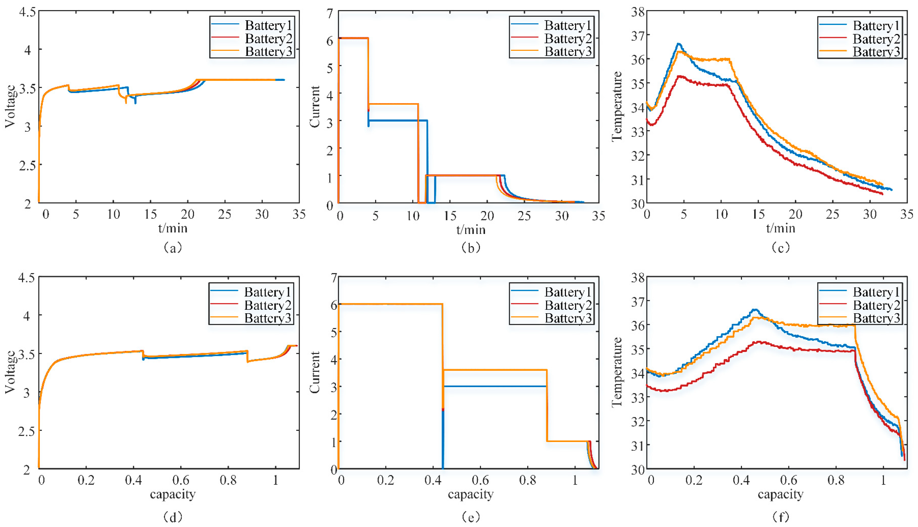
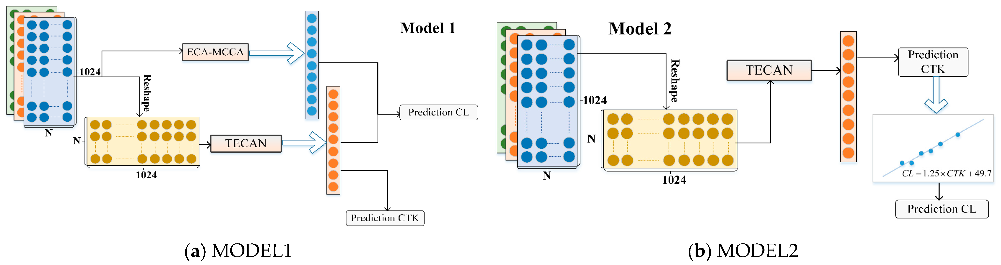
In this study, innovative research is conducted to construct more accurate lifetime prediction models by utilizing the spatial and temporal characteristics of multi-dimensional data parameters such as voltage (V), current (I), and temperature (T). A joint prediction architecture is proposed by systematically integrating TCN and ECA. At the feature extraction level, the ECA module is introduced to enhance the dynamic sensing capability of the TCN network for temporal features. At the prediction mechanism level, a CL-CTK collaborative prediction framework is innovatively constructed to effectively enhance the model’s ability to characterize the complex nonlinear relationships in the battery degradation process. This fusion strategy accurately captures the dynamic evolution law during battery aging through the synergistic optimization of multi-dimensional features. It demonstrates a significant improvement in prediction accuracy over the traditional single-model approach. The primary contributions of this paper are summarized as follows:

1. This paper designs and implements a spatial feature extraction module and a temporal feature extraction module, a framework that can efficiently extract key spatial and temporal features from the early V/I/T data of batteries, laying the foundation for subsequent prediction.

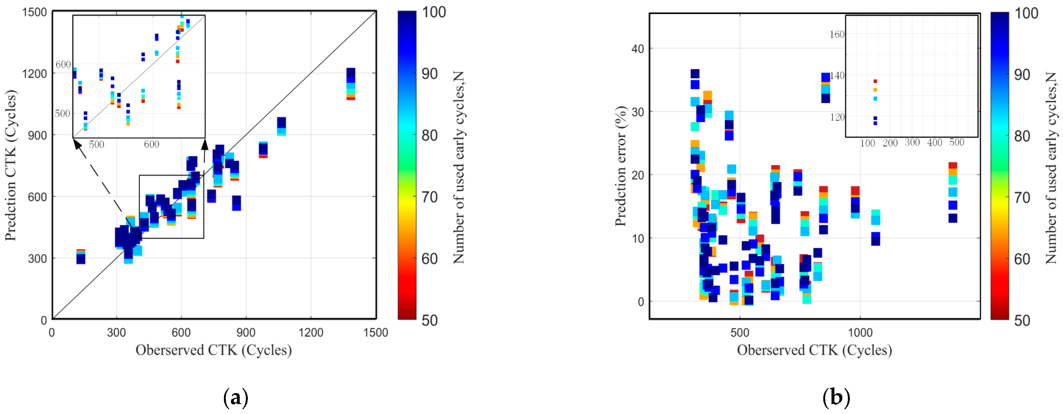
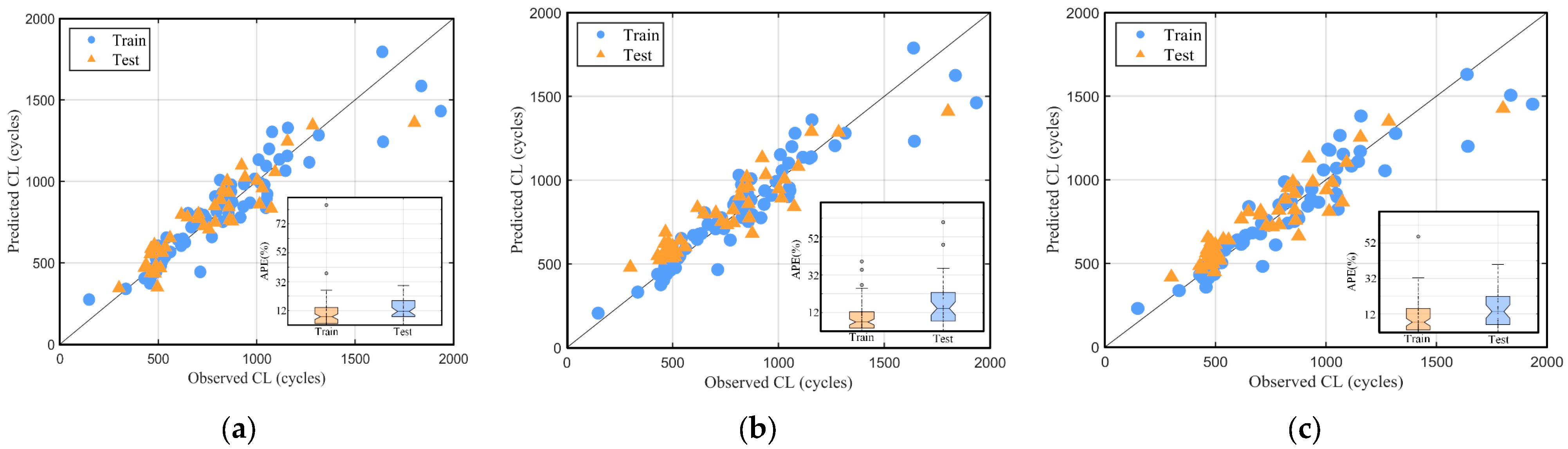
2. By integrating CTK prediction into the CL prediction process, this model effectively accounts for the nonlinear aging characteristics of the battery, significantly improving prediction accuracy. The experimental results indicate that the RMSE of the model on CL prediction is reduced to an error level of 106 cycles when utilizing data from the first 100 cycles of the battery.

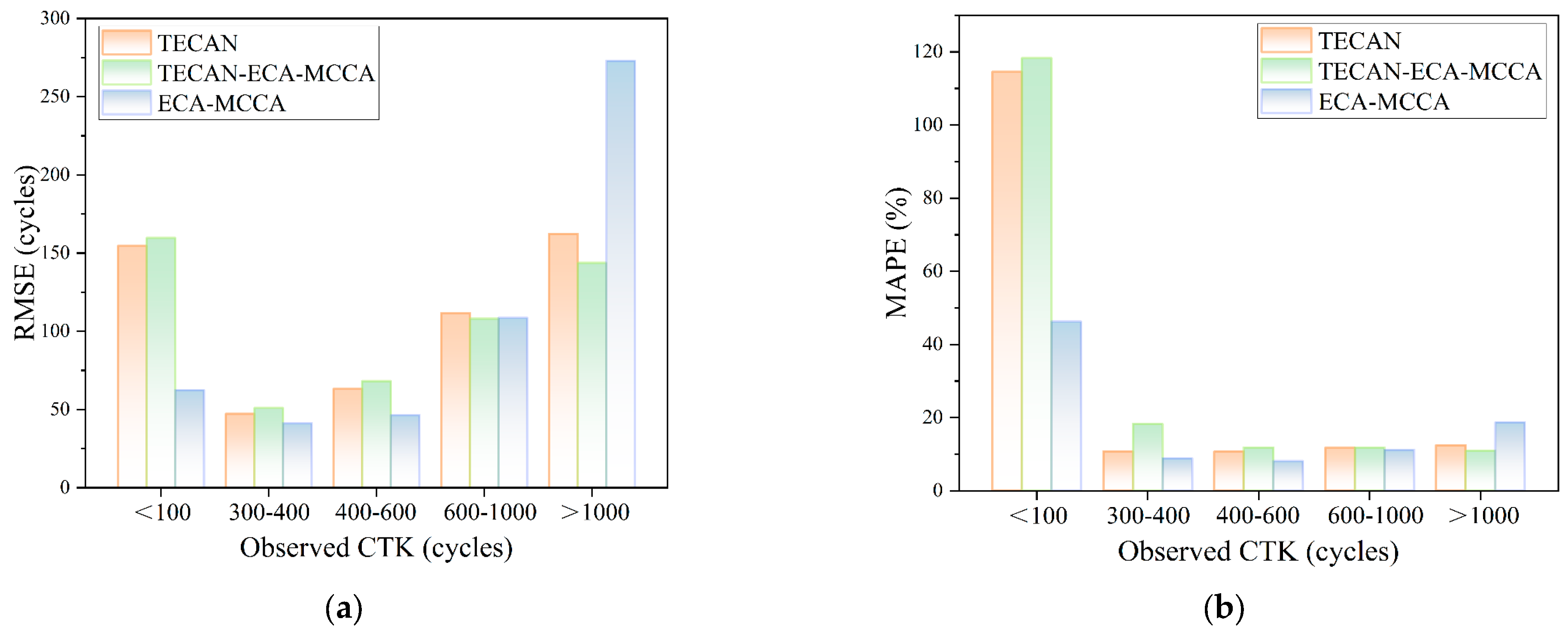
3. In this study, a joint prediction model is used and rigorously validated on the Stanford dataset. The experimental results show that combining TCN with ECA enhances the feature extraction capability of the model. Further, when this combined model is used for joint prediction with CTK, the predictive ability of the model is further improved.

The rest of the paper is organized as follows: Section 2 describes the relevant modules used in this paper. Section 3 discusses the dataset used in this paper and the model architecture used for battery CTK prediction and CL prediction. Section 4 includes evaluation metrics, experimental details, and experimental results, discussing the prediction results for CL and CTK, respectively. Finally, Section 5 includes conclusions.

2. Introduction of Related Modules

2.1. Efficient Channel Attention (ECA)

The efficient channel attention (ECA) module serves as a weight extraction mechanism for this study’s spatial and temporal feature extraction components [35]. This module was presented by Wang in 2019. Its primary function is to augment the model’s focus on critical features, thereby enhancing its capability to capture the battery’s early-stage spatial and temporal characteristics accurately. The detailed architecture of the ECA module is illustrated in Figure 1, which enhances the channel information without dimensionality reduction in the channels. Firstly, it goes through a global average pooling layer (GAP) to extract the comprehensive information of each channel, then applies a 1D convolutional layer to extract the information of local cross-channel interactions. Furthermore, ECA applies a dynamic convolutional kernel in the 1D convolutional layer to adjust the interactive coverage and reasonably capture the neighboring channel information. The convolution kernel size $k$ is calculated as follows:

$$k=\psi (C)={\left|{\displaystyle \frac{{\log }_2(C)}{\gamma }}+{\displaystyle \frac{b}{\gamma }}\right|}_{odd}$$

(1)

where $C$ is the number of channels in the one-dimensional convolutional layer in the ECA model, whose size has been scaled to 64 before the ECA model. $\gamma$ and $b$ are hyperparameters in the model, where $\gamma$ is set to 2 and $b$ is set to 1, whose sizes are determined based on previous experimental results. After convolution, the sigmoid layer is used to fix the values between [0, 1]. The weights corresponding to each channel are obtained and later multiplied with the original input feature map to achieve feature enhancement.

Figure 1. Efficient channel attention module framework.

2.2. Multi-Scale Charge Cycle Attention with Efficient Channel Attention Module (ECA-MCCA)

ECA-MCCA, as the spatial feature extraction module in this paper, is mainly used to extract the spatial features of the early charging cycle of the battery. Its structure is shown in Figure 2. The features extracted by this module can reflect the relationship between different battery cycles in the early stage and the relationship between charging voltage, charging current, and charging temperature in the same cycle. The feature extractor structure mainly consists of ECA and multi-scale charge cycle concern (MCCA). The data are first expanded using a 2D convolutional layer to fully extract the complex information implied by V/I/T. In this model, the formula for the 2D convolutional layer is shown in Equation (2) as follows:

$${{\displaystyle u}}_{i,j}={\displaystyle \sum _{m=0}^{\mathrm{k}\_h-1}{\displaystyle \sum _{n=0}^{\mathrm{k}\_w-1}{\displaystyle \sum _{c=0}^{in\_ch-1}{I}_{i+m,j+n,c}\cdot W_{m,n,c}+B}}}$$

(2)

where ${{\displaystyle u}}_{i,j}$ denotes the value of position $(i,j)$ on the output feature map. $k\_h$ and $k\_w$ are the height and width of the convolution kernel, respectively. $in\_ch$ denotes the number of channels of the input feature map. $I_{i+m,j+n,c}$ denotes the value of position $(i+m,j+n)$ on the input feature map, and the channel is $c$. $W_{m,n,c}$ denotes the weight on the convolution kernel at position $(m,n)$ and corresponding to channel $c$ of the input feature map. $B$ denotes the bias term, which is a learnable parameter used to adjust the range of values of the output feature map.

Figure 2. Architecture of the spatial feature extraction module ECA-MCCA.

As shown in Figure 2, to obtain the relationship between voltage, current, and temperature at the same charging capacity point, the ECA is applied after the 2D convolutional layer. ECA not only gives higher weights to the channels with higher correlation but also applies a 1D convolutional layer to extract the local cross-channel interaction information, effectively extracting the interaction features between voltage, current, and temperature.

The right side of Figure 2 details the architecture of the MCCA, which consists of three uniformly constructed combinatorial modules, and the ECA-processed data are fed into each module in parallel to extract spatial features at different scales. Each module contains an inflated convolutional layer, a criss-cross attention block (CC Block), and two activation functions. The key difference between these three modules is the different expansion coefficients used in their expansion convolutional layers, specifically [1, 2, 5]. These differentiated expansion coefficients enable multi-scale perceptual fields, which capture multi-scale information from the battery’s charge-cycle-to-capacity ratio.

Such multi-scale features can reveal the intrinsic connection between different capacity points, thus effectively extracting the spatial characteristics of the early data from the capacity ratio curves. After the data are processed through the inflated convolutional layer, they enter a criss-cross attention block (CC Block) responsible for capturing the global information. This block not only extracts the correlation information between capacity points and cycles but also superimposes features containing neighboring information on the original feature map, facilitating feature gain between related features and achieving effective feature enhancement.

Then, in order to estimate the correlation between the multi-scale information and the battery life prediction results, a two-layer perceptron is used to model the multi-scale charging cycle attention score $S_n$, which is calculated as shown in Equation (3):

$$S_n=f\left({\displaystyle \sum _{j=1}^{n_{CA}}{v}_n^{j}g\left({\displaystyle \sum _{i=1}^{I_n}{z}_n^{i,j}{O}_n^i+b_n^j}\right)+c_n}\right),n=1,2,3.$$

(3)

where $I_n$ is the number of elements of the inflated convolutional feature map after global average pooling, and $z_n$ and $b_n$ are the weights and biases of the first perceptron layer, respectively. $v_n$ and $c_n$ are the weights and biases of the second perceptron, respectively. Here, $n_{CA}$ is a hyperparameter that is the dimension of the intermediate representation of the transformation. $g(-)$ and $f(-)$ are the hyperbolic tangent function and S-shaped function, which are used to perceive the battery aging information implied by the feature map at different scales.

Next, in order to compare the importance of the aging information at different scales, the multi-scale charging cycle attention score $S_n$ that has passed through the two layers of perceptron will be normalized to obtain its importance score ${\omega }_{S_n}$. After that, as shown in Equation (4), the data $O_n$ after the CC Block will be multiplied with ${\omega }_{S_n}$ to obtain the final spatial feature extraction data $P_n$.

$$P_n={\omega }_{S_n}\cdot O_n={\displaystyle \frac{S_n}{{\displaystyle {\sum }_{l=1}^3{S}_l}}}\cdot O_n,n=1,2,3.$$

(4)

In this way, spatial information at different scales will contain corresponding weights in the final result. Finally, as shown in Equation (5), at the output of the MCCA module, we employ the concatenate operation to integrate the multi-scale features and obtain the spatial features of the early data.

$$SC=concatenate((P_1,P_2,P_3),axis=0)$$

(5)

2.3. Temporal Efficient Channel Attention Network (TECAN)

This paper’s temporal feature extraction module employs a temporal efficient channel attention network (TECAN). As shown in Figure 3, this module is derived from the temporal convolutional network (TCN) and achieves a more efficient capture of temporal information by incorporating the ECA weighting module [14]. TCN is a new type of temporal convolutional network distinguished from RNN and LSTM. It employs dilated causal convolution (DCC) and residual networks to overcome the limitations of traditional CNN in capturing long-term temporal dependencies from time series data. Specifically, DCC leverages the parallel training capabilities of CNNs to enhance the efficiency of TCN in processing historical information. As illustrated in Figure 4, it utilizes causal convolution to capture historical data, although the size of the convolution kernel constrains the extent of pure causal convolution for this purpose. To capture more historical information, it is necessary to stack multiple layers of causal convolution. In order to efficiently obtain more receptive fields without adding causal convolutional layers, TCN employs sequentially incremental inflated convolutional coefficients to expand the receptive field, thereby progressively obtaining more extended history information. Furthermore, to ensure that the dimensions of the inputs and outputs remain constant, the sequence is expanded using padding, which grows in size as dilation grows, as shown in the Equation (6) as follows:

$$Padding=(k-1)\ast d$$

(6)

Figure 3. The architecture of the temporal feature extraction module TECAN.

Figure 4. A stack of dilated causal convolutions with convolution kernel size k = 3 and dilation factors d = 1, 2, 5.

The specific operation of convolution is shown in Equation (7) as follows:

$$F\left(s\right)=\left(X\ast {}_{d}f\right)(s)={\displaystyle \sum _{i=0}^{k-1}f(i)\cdot X_{s-d\cdot i}}$$

(7)

where $k$ is the size of the convolution kernel, in this study the size is [1, 8], and $\ast$ is the convolution operator. The subscript $s-d\cdot i$ stands for the direction of the past, and $d$ is the dilated factor.

In this paper, in order to make sure that TCN can adaptively highlight the compelling features, we design TECAN as shown in Figure 3, and the ECA module calculates the corresponding weights for each channel. Then, the weight values are multiplied with the deep features extracted by the two layers of DCC, effectively making the module adaptive to focus on information containing more aged features. Finally, the enhanced features are then summed with the input features to obtain the final output features, which are calculated as shown below

$${\tilde{F}}_T=F_T\oplus \left({\widehat{F}}_T\otimes {\omega }_T\right)$$

(8)

where $F_T$ is the input feature and ${\widehat{F}}_T$ is the depth feature extracted by the two-layer DCC. ${\omega }_T$ denotes the weight parameter of all the channels learned by the ECA. ${\tilde{F}}_T$ is the final output feature. $\otimes$ denotes the multiplication of the channel direction, and $\oplus$ denotes the addition of the channel direction. From the above analysis, it can be seen that TECAN is not only effective in extracting historical information but also improves the feature enhancement capability, which is not available in TCN.

3. Data Processing and Simulation Verification

3.1. Dataset and Label

3.1.1. Dataset Description

The battery dataset in this paper comes from accelerated aging tests conducted by Severson [36]. It comprises 124 lithium-ion phosphate (LFP)/graphite cells manufactured by A123 Systems (APR18650M1A). All the batteries involved in the test were in the same initial state before the test, and all were tested under the same temperature conditions. Their specific conditions are shown in Table 1. Five of the batteries had problems with capacity increase due to storage time, so only the remaining 119 batteries were used as input data for the model.

Table 1. Technical specifications of experimental LIBs.

Manufacturer	A123 Systems
Type	APR18650M1A
Cathode/Anode	LiFePO4/Graphite
Rated capacity/Rated voltage	1.1 Ah/3.3 V
Upper voltages/Cut-off voltages	3.6 V/2 V
Environmental temperature	30 °C
Charging mode	C1(Q1)-C2-CV
Discharging current	4 C (4.4 A)

A total of 72 different charging strategies were used for the batteries in this study. All batteries followed a constant current–constant voltage (CC-CV) charging pattern. Specifically, the constant current charging stage is categorized into a one-step or two-step fast charging method, denoted as C1(Q1)-C2. In this denotation, C1 stands for the current multiplication rate of the first charging step, and C2 stands for the current multiplication rate of the second charging step. Both of them take values ranging from 3.6 C to 6 C. Q1, indicating the state-of-charge of the batteries when they are switched from the first charging step to the second charging step. It is worth noting that the second step of the constant current charging process will be terminated when the battery reaches 80%, after which the battery will rest for one minute.

After the rest, the battery enters the CC stage at a 1 C times rate until its voltage reaches the preset upper cut-off voltage of 3.6 V. After reaching this voltage, the charging mode is switched to constant voltage charging, i.e., charging at a constant voltage of 3.6 V until the charging current decays to zero.

During the discharge cycle phase, each battery is discharged at a constant current of 4 A until the battery voltage drops to 2 V. Subsequently, the discharge mode is changed to discharge at a constant voltage of 2 V until the discharge current decreases to 0.02 C, marking the end of the discharge process.

Cycle life (CL) is the number of charge and discharge cycles performed when the battery reaches an 80% state of health (i.e., 0.88 Ah). As shown in Figure 5, the CL in this dataset ranges from 150 to 2000 cycles. Eighty-five percent of the total dataset has a CL between 400 and 1000 cycles, and 400 to 600 cycles account for about 35%. Only one battery in this dataset has a CL of less than 200 cycles.

Figure 5. CL distribution of LIBs.

3.1.2. Input Data Generation

In Figure 6, parts (a) through (c) show the relationship between battery charging time and charging voltage (V), charging current (I), and temperature (T) when time is used as the independent variable. It can be observed that when time is used as the independent variable and the V/I/T values of the battery are input into the model, it is difficult to avoid the potential influence of time on the predicted results due to the charging strategy. Specifically, during constant current charging, different charging strategies result in differences in charging time, which may influence the charging strategy’s predicted battery results.

Figure 6. Charging V, I, and T of three batteries with different charging strategies. (a) Time–charge voltage; (b) Time–charge current; (c) Time–temperature; (d) Charging capacity–charge voltage; (e) Charging capacity–charge current; (f) Charging capacity–temperature.

To overcome this limitation, we used input data with charging quantity as the independent variable. As shown in Figure 6dȓf, this approach effectively avoids potential effects due to timing issues. By using the charging amount as the independent variable, we can more directly reflect the battery’s performance changes, thus reducing the interference of different charging strategies on the prediction results. This approach improves the accuracy of the prediction and enhances the reliability of the prediction results.

In this prediction model, the first N cycles are used as input data for the model. Data cleaning should be required first. The charged V/I/T data with the exact dimension of 1024 sampling points were extracted from the original data using nearest neighbor interpolation, and the data were normalized using 0–1 normalization. In this way, the characteristics of the battery state over cycles and all the features hidden in the V/I/T curve can be fed into the model in a more standardized form. The N cycles of the battery are fused into a matrix to extract the temporal characteristics and multi-scale features of the battery.

When extracting features from battery spatial characteristics, the input data should be of dimensionality (76, 3, N, 1024), where the first dimension represents the number of batteries, the second dimension encompasses early battery features such as V/I/T, the third dimension denotes the number of early cycles for each battery, and the fourth dimension indicates the number of sampling points per charge cycle. In the temporal feature module, the V/I/T are simultaneously fused, transforming the input data scale to (76, 1, 1024, N). Here, the first dimension still represents the number of batteries; the second dimension now represents the fused feature; the third dimension indicates the number of sampling points per charge cycle; and the fourth dimension denotes the number of early cycles for each battery.

3.1.3. Linear Relationship Between Knee Point and Life Prediction

As shown in Figure 7a, it is generally accepted that the knee point is the turning point in the battery’s aging process from a smooth decline to rapid aging [37]. Many methods have been proposed to perform recognition calculations on knee points. The commonly used methods are the needle model [38], the Bacon–Watts model [39], the tangent-ratio model [40], and the bisector model [41].

Figure 7. Battery cycling data of the dataset. (a) The capacity fade trajectories of the selected batteries; (b) The knee point identification based on the bisector model on a capacity fade trajectory of one cell; (c) CTK and EOL distribution of the batteries.

This paper uses the bisector model to obtain the CTK, as shown in Figure 7b. Firstly, a fifth-degree polynomial is defined as

$$y=p_0+p_{1}x+p_2{x}^2+p_3{x}^3+p_4{x}^4+p_5{x}^5$$

(9)

which is used to fit the relationship between the number of battery cycles and its discharge capacity. Two straight lines with different slopes from the Bacon–Watts model are then used to fit the decay trajectories at the start and end points of the battery life, namely

$$Y=a_0+a_1\left(x-x_0\right)+a_2\left(x-x_0\right)\tanh \left\{{\displaystyle \frac{\left(x-x_0\right)}{\eta }}\right\}+Z$$

(10)

where $\eta =1\times {10}^{-8}$, $Z$ is a normally distributed residual value, $(x_0,a_0)$ is the intersection of the two lines, and $a_1$ and $a_2$ are used to control the slopes of the two lines to obtain a better fit. Then, we calculate the equation of the angle bisector of the two lines as follows:

$$y=k(x-x_0)+a_0$$

(11)

$$k=\left\{\left(1-{\beta }_1{\beta }_2\right)-\sqrt{{({\beta }_1{\beta }_2-1)}^2+{({\beta }_1+{\beta }_2)}^2}\right\}/({\beta }_1+{\beta }_2)$$

(12)

$${\beta }_1=a_1-a_2$$

(13)

$${\beta }_2=a_1+a_2$$

(14)

where ${\beta }_1,{\beta }_2$ are the slopes of the two lines, respectively. Finally, the coordinates of the knee point $(x,y)$ obtained by the joint solution of Equations (9) and (11), where $x$ denotes the CL when the knee point is reached, and $y$ denotes the discharge capacity corresponding to the knee point.

From Figure 7c, it can be seen that CL and CTK have a strong linear relationship; its Pearson’s correlation coefficient is 0.9931, which can be seen by fitting CL and CTK with a linear fitter as follows:

$$CL=1.25\times CTK+49.7$$

(15)

The high correlation between CTK and CL is an important basis for the joint prediction model in this paper. Therefore, CTK can be considered a critical and reliable basis for making predictions about CL.

3.2. Joint Modeling of Early Prediction of Knee Point and Cycle Life

To validate our model’s predictive capabilities, we thoroughly trained it and tested it on 43 batteries exhibiting diverse CL and charging strategies. Initially, we independently employed the ECA-MCCA temporal and TECAN spatial modules to forecast CL and CTK. Concurrently, we explored the synergistic effects of combining these modules to enhance prediction accuracy. Building upon this, we innovatively introduced two hybrid models, MODEL1 and MODEL2, designed explicitly for joint CL and CTK forecasting. Notably, by integrating CTK prediction as an intermediary step, we harnessed the nonlinear aging characteristics of batteries to refine CL predictions further. Effectively capturing the nonlinear aging feature means that the models in this paper can further improve their ability to predict the lifetime by making a good prediction of the CTK. Our experiments varied the initial number of cycles, N, to examine its impact on forecasting outcomes. The performance of the combined model was validated by comparing it with other models.

When adjusting the hyperparameters, the dynamic convolution kernel of the ECA module is set to 5, and the three dilated convolution layers of the MCCA have convolution coefficients of [1, 2, 5]. In the temporal feature extractor species, the one-dimensional convolutional layer of TCN is changed to a two-dimensional convolutional layer to feed the four-dimensional data into TECAN for training reasonably. The number of channels of each expansion convolutional layer is set to [16, 32, 64], the convolutional kernel size is set to [1, 8], the step size is set to [1, 1], and the padding is set to [0, padding]. In addition, the kernel size and step size for each convolutional or maximum pooling layer were chosen empirically. The slope of the ReLU activation function was set to 0.1 by default. The maximum number of training periods was set to 450. An Adam optimizer with a learning rate of 1 × 10⁻⁵ was used to update the weights.

Models with Nonlinear Aging Features

The primary focus of this paper is to accurately predict battery life by utilizing CTK, which reflects the nonlinear aging characteristics of batteries. The primary focus is on optimizing and improving the TECAN module. Specifically:

In MODEL1, shown in Figure 8a, we adopt the innovative ECA-MCCA-TECAN framework, which combines the spatial and temporal features of early data. The ECA-MCCA component extracts spatial features, while TECAN extracts temporal attributes. The novelty of this design is the integration of CTK as a label into the TECAN framework, which enhances TECAN’s ability to learn the nonlinear aging characteristics of batteries.

Figure 8. CL prediction model with the addition of CTK prediction (a) MODEL1: ECA-MCCA model with CTK prediction; (b) MODEL2: TECAN model with CTK prediction.

In MODEL2, as depicted in Figure 8b, the prediction is solely performed using the TECAN module, focusing on utilizing temporal features. The model first precisely predicts the CTK through the TECAN module. Subsequently, the CL is further derived based on the established mathematical relationship between the CL and CTK, as shown in Equation (15). This approach not only simplifies the prediction process but also makes full use of the intrinsic link between the CTK and the battery life, aiming to achieve more accurate predictions.

4. Experimental Verification and Comparative Analysis

4.1. Evaluation Metrics

In this model, the mean square error (MSE) of the prediction result is used as the loss function, and the Adam optimizer is applied to adaptively adjust the learning rate to find the minimum value of the loss function. In evaluating the performance of the model as well as its predictive effectiveness, the root mean square error (RMSE), mean absolute error (MAE), mean absolute percentage error (MAPE), symmetric mean absolute percentage error (SMAPE), coefficient of determination ($R^2$), and absolute error (AE) are applied to evaluate the predictive performance of the model. The formulas are shown below:

$$MSE={\displaystyle \frac{1}{n}}{\displaystyle \sum _{i=1}^n{({\widehat{y}}_i-y_i)}^2}$$

(16)

$$RMSE=\sqrt{{\displaystyle \frac{1}{n}}{\displaystyle \sum _{i=1}^n{({\widehat{y}}_i-y_i)}^2}}$$

(17)

$$MAE={\displaystyle \frac{1}{n}}{\displaystyle \sum _{i=1}^n\left|{\widehat{y}}_i-y_i\right|}$$

(18)

$$MAPE={\displaystyle \frac{100\%}{n}}{\displaystyle \sum _{i=1}^n\left|\frac{{\widehat{y}}_i-y_i}{y_i}\right|}$$

(19)

$$AP{E}_i={\displaystyle \frac{\left|y_i-{\widehat{y}}_i\right|}{y_i}}\times 100$$

(20)

$$R^2=1-{\displaystyle \frac{{\displaystyle {\sum }_{i=1}^n{(y_i-{\widehat{y}}_i)}^2}}{{\displaystyle {\sum }_{i=1}^n{(y_i-{\overline{y}}_i)}^2}}}$$

(21)

where ${\widehat{y}}_i$ is the predicted value, ${\overline{y}}_i$ is the average of the true values, $y_i$ is the true value, and $n$ is the number of samples.

4.2. Result and Discussion

4.2.1. Results of Timing and Spatial Characteristics for CTK Prediction

In order to more accurately predict battery life using the battery knee point, this paper pioneers the introduction of the temporal model TECAN, the spatial model ECA-MCCA, and the spatiotemporal fusion of the two, TECAN-ECA-MCCA. By employing the three aforementioned models to predict CTK, an optimal model combination strategy is determined for correlating battery knee points with aging lifespan. The specific results of CTK prediction are detailed in Table 2, and the data clearly show that in terms of prediction accuracy, the TECAN model, which is good at capturing temporal features, as well as the TECAN-ECA-MCCA model, which fuses temporal and spatial information, have lower RMSE than the ECA-MCCA model.

Table 2. CTK prediction results for temporal, spatial, and spatiotemporal models.

MODEL	RMSE (Cycles)	MAE (Cycles)	MAPE (%)	${\mathit{R}}^2$ (%)
TECAN	88.25	66.18	13.57%	86.56%
TECAN-ECA-MCCA	89.52	68.22	14.35%	86.93%
ECA-MCCA	93.58	61.66	10.88%	84.88%

Considering the wide range of values between CL and CTK in the sample of batteries used in this study, coupled with the high sensitivity of MAPE to slight differences, this property may inadvertently amplify the effect of errors on smaller actual values. Therefore, RMSE was chosen as the primary assessment metric in this study. This choice is further substantiated by an exhaustive comparative analysis of battery datasets spanning various magnitudes, illustrated in Figure 9b; except for individual abnormal data points with CTK less than 100, all standard data showed good predictive accuracy.

Figure 9. Comparison of results of TECAN, TECAN-ECA-MCCA, and ECA-MCCA models for different battery CL. (a) Comparison of root mean square errors; (b) Comparison of mean absolute percentage errors.

This paper innovatively proposes incorporating knee point features into the time-series model TECAN to optimize battery life prediction. Finally, prediction models MODEL1 and MODEL2 based on the knee joint are constructed.

As can be seen in Figure 10, Figure 10a is a comparison plot when using the TECAN model to predict CTK, Figure 10b is a comparison plot when using the TECAN-ECA-MCCA model to predict CTK, and Figure 10c is a comparison plot when using the ECA-MCCA model to predict CTK. It can be found that the ECA-MCCA model exhibits high prediction accuracy when the number of battery cycles is below 1000 cycles. However, when the number of cycles exceeds 1000, the prediction effect is significantly lower than that of the TECAN model. Based on this finding, CTK prediction using the TECAN model prior to CL prediction can be more effective in classifying and predicting CL. This approach not only improves prediction accuracy but also provides more accurate and timely guidance for battery management.

Figure 10. Observed CTK and predicted CTK for the training and test sets. (a) TECAN model CTK prediction results; (b) TECAN-ECA-MCCA model CTK prediction results; (c) ECA-MCCA model CTK prediction results. The inset shows the APE distribution for the training and test data.

The data in Table 3 show the prediction performance of the TECAN model for CTK under different N conditions, and the prediction effect is better as N increases. Figure 11 shows the TECAN model’s performance for each cell’s prediction ability in the test set. In Figure 11b, we have presented it separately as an inset to avoid significant errors in one cell interfering with the clear presentation of data from other cells. Therefore, in practical applications, the model can gradually improve the prediction accuracy by increasing the cyclic data in the running process.

Table 3. Prediction results for CTK using the TECAN model have a certain N.

N	RMSE (Cycles)	MAE (Cycles)	MAPE (%)	${\mathit{R}}^2$ (%)
50	100.26	72.63	14.84%	83.15%
60	97.94	70.61	14.51%	83.77%
70	96.53	70.04	14.54%	84.26%
80	93.28	69.86	14.51%	85.02%
90	91.50	69.17	14.42%	85.59%
100	86.92	67.83	14.27%	86.33%

Figure 11. Predictions of CTK using the TECAN model with some N. (a) Comparison of root-mean-square error; (b) Comparison of mean absolute percentage error.

4.2.2. Results of Predicting CL Based on Temporal and Spatial Characteristics

Table 4 comprehensively presents the performance of three models—ECA-MCCA, TECAN, and TECAN-ECA-MCCA—for CL prediction with N = 100. The analysis reveals that both spatial and temporal features of early battery characteristics play a crucial role in CL prediction, demonstrating that the effective utilization of these early data can lead to accurate estimations of CL. Based on the data analysis presented in Table 4, it can be observed that only the ECA-MCCA model is used for prediction; the RMSE is 118.83 cycles; in contrast, the RMSE of the TECAN model is 130 cycles. Further, when we combine the ECA-MCCA model with the TECAN model to form the TECAN-ECA -MCCA fusion model, the fusion model significantly improves prediction performance compared to the original TECAN model. This result indicates that the spatial features of the battery exhibit superior prediction capability compared to the temporal features in the scenario of CL prediction using the early data. Notably, despite integrating both spatial and temporal features aiming to harness their combined strengths, the TECAN-ECA-MCCA model does not achieve the anticipated substantial improvement in predictive performance. In addition, due to the significant increase in model complexity, the time cost required for each round of training rises significantly accordingly. This phenomenon suggests that the relationship between model complexity and performance improvement does not show a desirable linear relationship under the existing framework.

Table 4. Comparison of the results of ECA-MCCA, TECAN, and TECAN-ECA-MCCA for CL prediction.

	ECA-MCCA	TECAN	TECAN-ECA-MCCA
RMSE (cycles)	118.83	130.40	120.85
MAE (cycles)	93.02	106.29	97.25
MAPE (%)	13.27	16.54	14.32
$R^2$ (%)	83.01	79.54	82.42
Time (s)	3.7	3.4	6.7

Figure 12 compares the training and testing sets’ observed CL and predicted CL for the three models listed in Table 4. Overall, the prediction performance shows a linear relationship. Batteries with CL values ranging from 400 to 1000 exhibit better predictive performance. In contrast, batteries with fewer training samples and CL values greater than 1500 demonstrate inferior predictive performance compared to those within the 400–1000 range. However, they can still be effectively distinguished from other batteries with CL values less than 1000.

Figure 12. Observed CL and predicted CL for the train sets and test sets. (a) ECA-MCCA model CL prediction results; (b) TECAN model CL prediction results; (c) TECAN-ECA-MCCA model CL prediction results. The inset shows the APE distribution of the training and test data.

4.2.3. Impact of Nonlinear Aging Characteristics on CL Prediction

The results from Table 4 indicate that early battery temporal characteristics are insufficient for accurately predicting CL, as they fail to effectively capture batteries’ inherent nonlinear aging properties. To address this limitation, this study introduces two models, MODEL1 and MODEL2, designed for the joint prediction of CL and CTK.

In order to verify the effectiveness of the model proposed in this paper, the prediction effectiveness of the model without CTK was compared with MODEL1 and MODEL2, and the comparison results are shown in Table 5. Table 5 illustrates that incorporating CTK prediction enhances model performance at N = 100. Specifically, in the TECAN, the RMSE without CTK prediction stands at 130 cycles, whereas it reduces to 106 cycles when CTK prediction is integrated into MODEL1. Furthermore, MODEL2 substantially enhances predictive accuracy when contrasted with MODEL1. This result further reveals that the nonlinear aging characteristics play a more central and significant role in predicting battery life. The predictive performances of MODEL1 and MODEL2 across varying N values are detailed in Table 6, respectively.

Table 5. Comparative results of CL prediction by models with and without CTK prediction added.

	RMSE	MAPE (%)	Time (s)
MODEL1	116.20	13.19	6.7
TECAN-ECA-MCCA	120.85	14.32	6.4
MODEL2	106.57	12.52	3.4
TECAN	130.40	16.54	3.4

Table 6. RMSE and MAPE for MODEL1 and MODEL2 for different ranges of battery CL for certain N.

Observed CL			50	60	70	80	90	100
<400	MODEL1	RMSE	145.38	140.58	126.55	125.91	78.67	76.54
		MAPE	48.46	46.86	42.18	41.97	26.22	25.51
	MODEL2	RMSE	149.18	142.28	134.51	135.23	115.05	119.18
		MAPE	49.73	47.42	44.84	45.08	38.35	39.73
400–500	MODEL1	RMSE	129.39	120.92	109.37	107.54	98.93	93.17
		MAPE	26.44	24.58	20.28	19.92	19.12	17.89
	MODEL2	RMSE	71.66	71.96	74.33	80.20	71.42	75.92
		MAPE	13.09	12.80	13.75	15.25	13.35	14.38
500–800	MODEL1	RMSE	116.69	107.16	93.60	92.47	81.17	73.56
		MAPE	15.30	14.04	12.14	11.99	10.88	9.77
	MODEL2	RMSE	84.79	86.04	84.30	86.70	70.00	74.33
		MAPE	11.80	11.91	11.75	11.90	8.95	9.86
800–1000	MODEL1	RMSE	134.35	123.32	135.7	134.05	124.89	117.74
		MAPE	14.31	12.75	13.77	13.60	13.12	12.15
	MODEL2	RMSE	86.10	89.15	85.09	89.75	112.00	117.74
		MAPE	7.44	8.10	7.69	8.26	11.60	12.51
1000–1300	MODEL1	RMSE	110.98	116.86	118.36	119.12	117.20	121.49
		MAPE	8.14	8.33	8.89	9.00	8.48	8.55
	MODEL2	RMSE	172.55	166.42	167.85	154.95	161.53	144.41
		MAPE	13.80	12.97	13.00	11.62	11.62	10.06
>1300	MODEL1	RMSE	299.00	335.15	325.28	336.12	388.76	410.96
		MAPE	16.6	18.61	18.06	18.66	21.58	22.82
	MODEL2	RMSE	389.25	371.70	352.87	320.42	284.50	248.63
		MAPE	21.61	20.64	19.59	17.80	15.80	13.80
TEST SET	MODEL1	RMSE	131.20	126.90	122.59	122.27	118.14	116.20
		MAPE	18.10	16.90	15.25	15.09	14.06	13.19
	MODEL2	RMSE	118.31	116.13	114.33	111.58	109.42	106.57
		MAPE	12.61	12.50	12.56	12.90	12.05	12.52

Based on the data analysis from Table 6, both models exhibit a significant reduction in RMSE with an increase in N, reflecting a notable improvement in predictive performance. Regarding evaluating prediction stability, the MAPE of MODEL1 decreases progressively as N increases, whereas MODEL2 remains relatively stable at approximately 12%, indicating better predictive consistency for MODEL2. Both models demonstrate effective feature extraction and learning capabilities for batteries with observed CL ranging from 400 to 1000. Specifically, within the CL range of 400 to 800, MODEL1’s predictive performance improves significantly with increasing N. In contrast, MODEL2 maintains more stable predictive outcomes, with its RMSE staying around 75 cycles, largely unaffected by changes in N. When considering batteries with CL exceeding 1300, the data reveal the impact of scarce training samples on predictive performance. Although neither model achieves optimal predictions for these highly aged batteries, they can effectively differentiate them from those with CL between 400 and 1000.

Comparative analysis of Figure 13a,c demonstrates the battery performance predictions of MODEL1 and MODEL2 under different N. Both models exhibit a significant linear correlation between the predicted CL and observed CL, with the prediction accuracy improving as N increases. Figure 13b,d illustrates the MAPE for individual batteries in the test set for MODEL1 and MODEL2, respectively. Notably, MODEL2 demonstrates superior stability in its predictions compared to MODEL1, as shown in Figure 13d.

Figure 13. Prediction results of CL using MODEL1 and MODEL2 with some N. (a) Comparison of RMSE of prediction results of MODEL1 on test set of 43 batteries; (b) Comparison of MAPE of prediction results of MODEL1 for the test set of 43 batteries; (c) Comparison of RMSE of prediction results of MODEL2 on test set of 43 batteries; (d) Comparison of MAPE of prediction results of MODEL2 for the test set of 43 batteries.

4.2.4. Comparative Experiment

To validate the model’s effectiveness further in this paper, we compared it with two existing models and four different neural network architectures, and the results are shown in Table 7. Among the two existing models, Zhang and Chen predicted the aging endpoint and aging trajectory of the battery using a MOGP and LSTM joint model, with an RMSE of 134 cycles at N = 100 [33]. Ma predicted the battery life using CNNs, with an average RMSE value of 127 cycles for both primary and secondary tests on the same dataset [32]. In contrast, after model training and testing using the same dataset, the results of the four neural network architectures are significantly inferior at N = 100, and the prediction results are shown in Table 7. In this paper, the proposed MODEL1 achieves an RMSE of 116 cycles at N = 100, and the RMSE of MODEL2 is even as low as 106 cycles, which shows higher prediction accuracy. In addition, the time required for each round of training for MODEL2 has increased compared to the base TCN network. However, its training time is significantly shorter than that of TIMESNET and Bi-LSTM networks. This result indicates that the models proposed in this paper achieve a better balance between prediction accuracy and computational efficiency and have high practical value.

Table 7. Comparison of battery life prediction methods.

	MSE (%)	RMSE (Cycles)	MAE (Cycles)	MAPE (%)	${\mathit{R}}^2$ (%)	Time (s)
MODEL2	0.50%	106.57	86.43	12.52%	86.33%	3.4
MOGP-LSTM [33]	-	134	-	7.87%	-	-
CNN [32]	-	127	-	5.1%	-	-
Bi-LSTM	1.19%	163.99	116.09	18.77%	67.64%	3.5
TCN	0.74%	128.93	105.89	17.47%	80%	3.2
TIMESNET	1.21%	164.65	135.61	20.93%	67.38%	3.7
LSTM	0.87%	140.27	114.49	18.72%	76.32%	3.4

5. Conclusions

By comparing the spatial and temporal characteristics of batteries in terms of prediction performance, we effectively evaluated the effectiveness of different models for battery life prediction. Experimental data revealed that using only early external temporal information for CL prediction fails to fully capture the complex nonlinear aging behaviors of batteries. To address this issue, our study introduced knee point features as a supplement, significantly enhancing the model’s ability to capture battery aging characteristics. Comparative analysis showed that combining CTK predictions with temporal features outperformed those based solely on early external temporal features in terms of accuracy and stability for battery life prediction. Notably, the TECAN temporal prediction model, after integrating CTK predictions, demonstrated the best prediction performance, with a significant improvement in prediction accuracy compared to other models.

References

1. Yuan, Y.; Yang, Q.; Ren, J.; Mu, X.; Wang, Z.; Shen, Q.; Wu, Z. Attack-defense strategy assisted osprey optimization algorithm for PEMFC parameters identification. Renew. Energy 2024, 225, 120211. [Google Scholar] [CrossRef]
2. Iqbal, R.; Liu, Y.; Zeng, Y.; Zhang, Q.; Zeeshan, M. Comparative study based on techno-economics analysis of different shipboard microgrid systems comprising PV/wind/fuel cell/battery/diesel generator with two battery technologies: A step toward green maritime transportation. Renew. Energy 2024, 221, 119670. [Google Scholar] [CrossRef]
3. Wang, X.; Zhu, H.; Luo, X.; Chang, S.; Guan, X. A novel optimal dispatch strategy for hybrid energy ship power system based on the improved NSGA-II algorithm. Electr. Power Syst. Res. 2024, 232, 110385. [Google Scholar] [CrossRef]
4. Qiu, Y.; Wen, S.; Zhao, Q.; Zhang, B.; Wu, G.; Zhu, M. Multi-model deep learning-based state of charge estimation for shipboard lithium batteries with feature extraction and Spatio-temporal dependency. J. Power Sources 2025, 629, 235983. [Google Scholar] [CrossRef]
5. Nwesaty, J.; Bratcu, A.L.; Ravey, A.; Bouquain, D.; Sename, O. Robust Energy Management System for Multi-Source DC Energy Systems—Real-Time Setup and Validation. IEEE Trans. Control Syst. Technol. 2020, 28, 2591–2599. [Google Scholar] [CrossRef]
6. Argyrou, M.C.; Christodoulides, P.; Kalogirou, S.A. Energy storage for electricity generation and related processes: Technologies appraisal and grid scale applications. Renew. Sustain. Energy Rev. 2018, 94, 804–821. [Google Scholar] [CrossRef]
7. Harris, S.J.; Harris, D.J.; Li, C. Failure statistics for commercial lithium-ion batteries: A study of 24 pouch cells. J. Power Sources 2017, 342, 589–597. [Google Scholar] [CrossRef]
8. Vennam, G.; Sahoo, A. A Dynamic SOH-Coupled Lithium-Ion Cell Model for State and Parameter Estimation. IEEE Trans. Energy Convers. 2023, 38, 1186–1196. [Google Scholar] [CrossRef]
9. Kim, T.; Adhikaree, A.; Pandey, R.; Kang, D.; Kim, M.; Oh, C. An On-Board Model-Based Condition Monitoring for Lithium-Ion Batteries. IEEE Trans. Ind. Appl. 2019, 55, 1835–1843. [Google Scholar] [CrossRef]
10. Lu, J.; Xiong, R.; Tian, J.; Wang, C.; Hsu, C.; Tsou, N.; Sun, F.; Li, J. Battery degradation prediction against uncertain future conditions with recurrent neural network enabled deep learning. Energy Storage Mater. 2022, 50, 139–151. [Google Scholar] [CrossRef]
11. Ma, G.; Zhang, Y.; Cheng, C.; Zhou, B.; Hu, P.; Yuan, Y. Remaining useful life prediction of lithium-ion batteries based on false nearest neighbors and a hybrid neural network. Appl. Energy 2019, 253, 113626. [Google Scholar] [CrossRef]
12. Zhang, Y.; Xiong, R.; He, H.; Pecht, M.G. Long short-term memory recurrent neural network for remaining useful life prediction of lithium-ion batteries. IEEE Trans. Veh. Technol. 2018, 67, 5695–5705. [Google Scholar] [CrossRef]
13. Ge, Y.; Ma, J.; Sun, G. A structural pruning method for lithium-ion batteries remaining useful life prediction model with multi-head attention mechanism. J. Energy Storage 2024, 86, 111396. [Google Scholar] [CrossRef]
14. Bai, S.; Kolter, J.Z.; Koltun, V. An Empirical Evaluation of Generic Convolutional and Recurrent Networks for Sequence Modeling. arXiv 2018, arXiv:1803.01271. [Google Scholar]
15. Tan, X.; Zhan, D.; Lyu, P.; Rao, J.; Fan, Y. Online state-of-health estimation of lithium-ion battery based on dynamic parameter identification at multi timescale and support vector regression. J. Power Sources 2021, 484, 229233. [Google Scholar] [CrossRef]
16. Xue, Z.; Zhang, Y.; Cheng, C.; Ma, G. Remaining useful life prediction of lithium-ion batteries with adaptive unscented kalman filter and optimized support vector regression. Neurocomputing 2020, 376, 95–102. [Google Scholar] [CrossRef]
17. Chen, L.; Ding, Y.; Liu, B.; Wu, S.; Wang, Y.; Pan, H. Remaining useful life prediction of lithium-ion battery using a novel particle filter framework with grey neural network. Energy 2022, 244, 122581. [Google Scholar] [CrossRef]
18. Li, S.; Fang, H.; Shi, B. Remaining useful life estimation of Lithium-ion battery based on interacting multiple model particle filter and support vector regression. Reliab. Eng. Syst. Saf. 2021, 210, 107542. [Google Scholar] [CrossRef]
19. Ma, L.; Tian, J.; Zhang, T.; Guo, Q.; Hu, C. Accurate and efficient remaining useful life prediction of batteries enabled by physics-informed machine learning. J. Energy Chem. 2024, 91, 512–521. [Google Scholar] [CrossRef]
20. Safitri, M.; Adji, T.B.; Cahyadi, A.I. Enhanced early prediction of Li-ion battery degradation using multicycle features and an ensemble deep learning model. Results Eng. 2025, 25, 104235. [Google Scholar] [CrossRef]
21. Sun, C.; Qu, A.; Zhang, J.; Shi, Q.; Jia, Z. Remaining Useful Life Prediction for Lithium-Ion Batteries Based on Improved Variational Mode Decomposition and Machine Learning Algorithm. Energies 2023, 16, 313. [Google Scholar] [CrossRef]
22. Wang, X.; Huang, T.; Zhu, K.; Zhao, X. LSTM-Based Broad Learning System for Remaining Useful Life Prediction. Mathematics 2022, 10, 2066. [Google Scholar] [CrossRef]
23. Goebel, K.; Saha, B.; Saxena, A.; Celaya, J.R.; Christophersen, J.P. Prognostics in Battery Health Management. IEEE Instrum. Meas. Mag. 2008, 11, 33–40. [Google Scholar] [CrossRef]
24. Li, F.; Xu, J. A new prognostics method for state of health estimation of lithium-ion batteries based on a mixture of Gaussian process models and particle filter. Microelectron. Reliab. 2015, 55, 1035–1045. [Google Scholar] [CrossRef]
25. Patil, M.A.; Tagade, P.; Hariharan, K.S.; Kolake, M.K.; Song, T.; Yeo, T.; Doo, S. A novel multistage support vector machine based approach for li-ion battery remaining useful life estimation. Appl. Energy 2015, 159, 285–297. [Google Scholar] [CrossRef]
26. Wang, D.; Miao, Q.; Pecht, M. Prognostics of lithium-ion batteries based on relevance vectors and a conditional three-parameter capacity degradation model. J. Power Sources 2013, 239, 253–264. [Google Scholar] [CrossRef]
27. Zhang, Y.; Xiong, R.; He, H.; Pecht, M. Validation and verification of a hybrid method for remaining useful life prediction of lithium-ion batteries. J. Clean. Prod. 2019, 212, 240–249. [Google Scholar] [CrossRef]
28. Chang, Y.; Fang, H.; Zhang, Y. A new hybrid method for the prediction of the remaining useful life of a lithium-ion battery. Appl. Energy 2017, 206, 1564–1578. [Google Scholar] [CrossRef]
29. Liu, D.; Zhou, J.; Pan, D.; Peng, Y.; Peng, X. Lithium-ion battery remaining useful life estimation with an optimized Relevance Vector Machine algorithm with incremental learning. Measurment 2015, 63, 143–151. [Google Scholar] [CrossRef]
30. Zheng, X.; Fang, H. An integrated unscented kalman filter and relevance vector regression approach for lithium-ion battery remaining useful life and short-term capacity prediction. Reliab. Eng. Syst. Saf. 2015, 144, 74–82. [Google Scholar] [CrossRef]
31. Zhang, F.; Shen, Z.; Xu, M.; Xie, Q.; Fu, Q.; Ma, R. Remaining useful life prediction of lithium-ion batteries based on TCN-DCN fusion model combined with IRRS filtering. J. Energy Storage 2023, 72, 108586. [Google Scholar] [CrossRef]
32. Ma, G.; Wang, Z.; Liu, W.; Fang, J.; Zhang, Y.; Ding, H.; Yuan, Y. A two-stage integrated method for early prediction of remaining useful life of lithium-ion batteries. Knowl. Based Syst. 2023, 259, 110012. [Google Scholar] [CrossRef]
33. Chen, Z.; Chen, L.; Ma, Z.; Xu, K.; Zhou, Y.; Shen, W. Joint modeling for early predictions of Li-ion battery cycle life and degradation trajectory. Energy 2023, 277, 127633. [Google Scholar] [CrossRef]
34. Yang, Y. A machine-learning prediction method of lithium-ion battery life based on charge process for different applications. Appl. Energy 2021, 292, 116897. [Google Scholar] [CrossRef]
35. Wang, Q.; Wu, B.; Zhu, P.; Li, P.; Zuo, W.; Hu, Q. ECA-Net: Efficient Channel Attention for Deep Convolutional Neural Networks. arXiv 2019, arXiv:1910.03151. [Google Scholar]
36. Severson, K.A.; Attia, P.M.; Jin, N.; Perkins, N.; Jiang, B.; Yang, Z.; Chen, M.H.; Aykol, M.; Herring, P.K.; Fraggedakis, D.; et al. Data-driven prediction of battery cycle life before capacity degradation. Nat. Energy 2019, 4, 383–391. [Google Scholar] [CrossRef]
37. IEEE Std 485-2020; IEEE Recommended Practice for Sizing Lead-Acid Batteries for Stationary Applications—Redline. Revision of IEEE Std 485-2010; IEEE: New York, NY, USA, 2020; pp. 1–99.
38. Satopaa, V.; Albrecht, J.; Lrwin, D.; Raghavan, B. Finding a “kneedle” in a haystack: Detecting knee points in system behavior. In Proceedings of the 2011 31st International Conference on Distributed Computing Systems Workshops (ICDCSW), Minneapolis, MN, USA, 25 July 2011. [Google Scholar] [CrossRef]
39. Fermín-Cueto, P.; McTurk, E.; Allerhand, M.; Medina-Lopez, E.; Anjos, M.F.; Sylvester, J.; Reis, G.D. Identification and machine learning prediction of knee-point and knee-onset in capacity degradation curves of lithium-ion cells. Energy AI 2020, 1, 10006. [Google Scholar] [CrossRef]
40. Diao, W.; Saxena, S.; Han, B.; Pecht, M. Algorithm to determine the knee point on capacity fade curves of lithium-ion cells. Energies 2019, 12, 2910. [Google Scholar] [CrossRef]
41. Greenbank, S.; Howey, D. Automated feature extraction and selection for data-driven models of rapid battery capacity fade and end of life. IEEE Trans. Ind. Inform. 2022, 18, 2965–2973. [Google Scholar] [CrossRef]
Disclaimer/Publisher’s Note: The statements, opinions and data contained in all publications are solely those of the individual author(s) and contributor(s) and not of MDPI and/or the editor(s). MDPI and/or the editor(s) disclaim responsibility for any injury to people or property resulting from any ideas, methods, instructions or products referred to in the content.
Article Metrics
Citations
Article Access Statistics
Multiple requests from the same IP address are counted as one view.