Abstract
The Wind Wall is a symmetric multi-VAWT system designed for efficient wind energy harvesting using Ugrinsky-type blades that are arranged in a compact, geometrically balanced layout to improve flow uniformity and torque stability and reduce pulsating loads. This study uses CFD simulations to determine the optimal helix angle and turbine spacing by analyzing the aerodynamic moment coefficient (), effective velocity (), and corresponding pressure-induced torque trends for stationary turbine configurations and proposes a simplified correlation linking , turbine diameter, and spacing. The results show that a helix angle of 20–30° and symmetric spacing yield the highest performance, with the optimal angle increasing the time-averaged by approximately 831% compared to the closest-packed case. These findings address the critical impact of improper spacing and sub-optimal twist angles in compact multi-turbine systems and provide the first combined CFD-based assessment of the helix angle and spacing for a symmetric Ugrinsky-blade Wind Wall, contributing a practical spacing–velocity relationship for future design and deployment.
1. Introduction
Energy is the main driving force behind the progress of humanity. The transition from muscle power to fire, then to coal, and from fossil fuels to electricity in the industrial age were the biggest turning points in human history [1,2,3,4,5,6]. Through energy, societies industrialize, living standards improve, and technology expands. However, the dependence on extinguishable sources of energy has caused numerous economic and environmental consequences. Air pollution, greenhouse gas released, and also global warming have always been the direct results of prolonged reliance on these sources [7,8,9]. Additionally, the limited nature of fossil-fuel available has raised concerns about providing energy in the long run and the sustainability of global development. Wind energy is one of the many ways in which we can extract clean energy from our surroundings. It is the process in which the kinetic energy in the wind particles flowing over a turbine is converted into mechanical energy by rotating the turbine blades, thus rotating the generator connected to them and producing electrical energy [1,10,11]. The generation of wind energy is primarily achieved through wind turbines, which are normally categorized into the horizontal-axis wind turbines or HAWTs and the vertical-axis wind turbines or VAWTs, as shown in Figure 1.
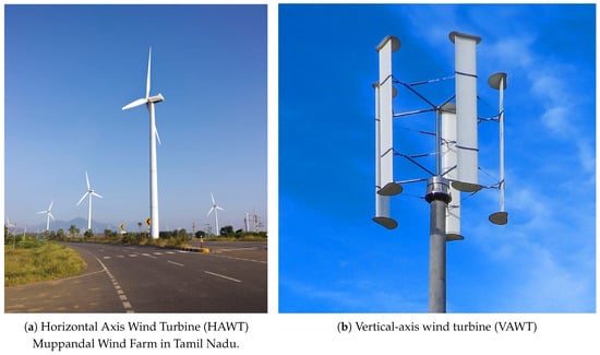
Figure 1.
Horizontal-axis and vertical-axis wind turbines.
The horizontal-axis wind turbines or ‘HAWTs’ are the most common type and are deployed in large-scale wind farms. Their blades rotate around a horizontal axis and must be aligned with the wind direction to function [12,13,14,15]. Although efficient in large-scale projects, they require tall towers, complex yaw systems, and considerable land area. Their main disadvantages are sensitivity to forecasted conditions, noise generated by the blades, and their visual and ecological impact (especially on birds) [1,16,17,18]. This issue, however, can be mitigated by decentralizing the production of wind power by using vertical-axis wind turbines (VAWTs), where the blades are arranged around a vertical axis. They capture wind from any direction without the need for orientation mechanisms. Their design allows for installation in urban areas and smaller spaces, often closer to places where energy is consumed. Their ability to function effectively in turbulent winds and operate at lower heights makes VAWTs a practical solution for decentralized energy production [19,20,21,22], allowing households, communities, and small enterprises to meet a portion of their energy needs sustainably.
Building upon these advantages of VAWTs, a design is proposed in this paper to maximize their performance and adaptability. This concept is the “Wind Wall,” which utilizes multiple vertical-axis turbines which are arranged in a series formation and put together in a compact frame to optimize energy capture. Unlike traditional stand-alone turbines, this configuration allows multiple VAWTs to work collectively, enhancing efficiency while minimizing land usage [19,23,24]. More recent studies have further investigated VAWT array aerodynamics and spacing-induced performance changes, particularly under turbulent and confined-flow conditions [25,26,27]. These works provide updated insights into turbine–turbine interaction mechanisms that directly relate to the Wind Wall configuration. The following section outlines the structural and functional aspects of this design.
The Wind Wall is a combination of Vertical-Axis Wind Turbines or VAWTs that are arranged in a frame that resembles a wall-like fence, as shown in Figure 2. It is designed in a way to extract the kinetic energy from the incoming wind and convert it into electrical energy. For our Wind Wall, the blade has a profile of the Ugrinsky type with a helical twist to enable operation at low wind speeds and reduced dependence on wind direction [28,29,30]. The Ugrinsky type of wind turbine falls under the group of drag-type turbines. These turbines operate by using the difference in drag on the two sides of the blade; one side of the turbine experiences less drag, while the other experiences more, creating an uneven force along the axis of the turbine. This force spins the blades and hence rotates the generator attached to it and produces power. By grouping the VAWTs in a frame, efficiency and power generation are increased, while the overall usage of available space is reduced.
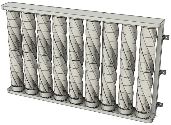
Figure 2.
Three-dimensional model of the turbines in a frame.
Symmetry plays an valuable role in the aerodynamic behavior of the Wind Wall. The Ugrinsky blade profile used in this study is geometrically symmetrical, ensuring that drag forces are distributed evenly along the rotating surface. Likewise, the turbines are arranged in a symmetric pattern inside the frame, allowing for uniform flow acceleration and balanced torque production among the neighboring turbines. This combination of blade symmetry and spatial symmetry contributes to smoother overall rotation, reduced vibration, and improved energy extraction compared to non-symmetric turbine arrays.
A vertical-axis wind turbine (VAWT) without a helical twist in its blades tends to experience torque fluctuations. For example, in a Savonius-type turbine with two or more blades, one blade may face the incoming wind, while the other faces in the opposite direction. This configuration produces alternating torque peaks, leading to a ripple-like variation in rotational motion, which prevents smooth operation. By introducing a helical twist to the turbine blades, the torque is distributed more evenly along the turbine height. The opposing aerodynamic forces acting on different sections of the blade are no longer directly in opposition, thereby producing a more constant torque and smoother rotation with fewer vibrations [28,31]. Increasing the helical twist improves torque uniformity; however, beyond a certain angle, the effective torque decreases, because the wind tends to deflect past the blades rather than applying useful momentum, thus reducing energy capture efficiency. Recent studies, including Reddy et al. (2023), have also emphasized the sensitivity of helical VAWT performance to both the twist angle and inter-turbine spacing, highlighting the importance of optimizing both parameters in clustered turbine configurations.
The blade profile used in this research is the Ugrinsky type as shown in Figure 3 and Figure 4, developed in the Soviet Union by Professor Ugrinsky and his team. This turbine design offers a balance between efficiency and starting capability, with reported power coefficients in the range of 0.25–0.35 [29,30]. The efficiency is greater than that of a pure Savonius-type turbine and comparable to certain Darrieus-type turbines. The Ugrinsky turbine therefore combines the self-starting ability of drag-based designs with the improved efficiency that is typically observed in lift-based turbines.
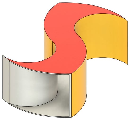
Figure 3.
Ugrinsky blade.
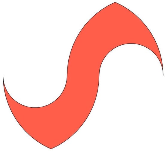
Figure 4.
Top view of the Ugrinsky blade profile.
In this study, the optimum helical twist (helix angle, as shown in Figure 5) is determined through Computational Fluid Dynamics (CFD) simulations by analyzing the torque generated at different twist angles under a constant wind speed. Once the optimum twist is identified, the ideal spacing between adjacent turbines in the Wind Wall is calculated. When turbines are positioned close together, the airflow between them accelerates due to the Venturi-like effect, as the same volume of air is forced through a narrower spacing. This acceleration is consistent with Bernoulli’s principle and results in higher effective wind speeds acting on the turbines [25,26,32,33]. Such acceleration phenomena and wake–wake interactions have also been observed experimentally in recent VAWT array studies, reinforcing the importance of spacing optimization for maximizing power extraction. The results of this work are later compared with relevant experimental and numerical studies in the literature to contextualize the aerodynamic behavior of the proposed Wind Wall system.
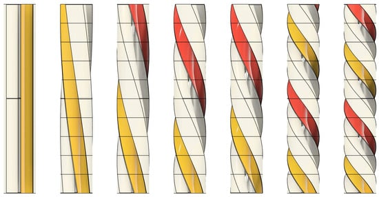
Figure 5.
Turbines with different helix angles; from left to right, the angles are 0°, 10°, 20°, 30°, 40°, 50°, and 60°.
It is important to note that the present study focuses exclusively on the aerodynamic behaviour of the Wind Wall, with particular attention to the torque–helix–spacing relationship obtained through CFD simulations. Structural considerations such as stress concentrations at blade–hub interfaces, fatigue behaviour under cyclic loading, manufacturability of helical Ugrinsky blades, and large-scale deployment constraints are not evaluated within this work. These aspects, while critical for practical implementation, require a dedicated structural and material analysis and will be investigated in future studies.
2. Problem Statement
The overall efficiency of the vertical-axis wind turbines can be significantly influenced by their blade geometry and the aerodynamic interference between adjacent units. Therefore, optimizing the helix angle and turbine spacing is crucial for improving energy capture and ensuring stable operation in compact wind wall arrays. The primary main goals of this research are given below:
- To determine the optimum helical twist(angle) of a single VAWT [12,34].
- To identify the optimum spacing between turbines arranged within the wind wall frame [19,35].
- To establish a correlation between the effective velocity of airflow through adjacent turbines and the spacing between them. This correlation is explained through the Venturi-like effect, in which airflow accelerates between narrow spacing according to the Bernoulli’s principle [36].
The helical twist of the turbine blades plays a central role in this investigation. As previously discussed, the introduction of a twist reduces torque fluctuations and produces smoother rotation [37]. Identifying the most effective helix angle is therefore critical, as it directly affects turbine efficiency and the consistency of power generation [38].
The computational study is thereby conducted using the Computational Fluid Dynamics (CFD) simulations [39]. A single turbine with measured height of 1 m and diameter of 0.17 m was modeled. The performance was evaluated at a constant wind speed of 8 m/s for helix angles of 0°, 10°, 20°, 30°, 40°, 50°, and 60°. Once the optimum helix angle was identified, a multi-turbine configuration was simulated to analyze the effect of spacing [40]. The spacing between turbines were varied as 0 cm, 0.5 cm, 1.66 cm, 4 cm, 7 cm, 11 cm, and 16 cm. These values were selected to cover both closely spaced and widely separated configurations, allowing the effect of turbine interaction to be captured effectively.
3. Numerical Methodology
3.1. Mathematical Formulations
This computational analysis for this research was carried out using the Reynolds-Averaged Navier–Stokes (RANS) equations in combination with standard wall functions of the turbulence model k-, and the mesh was generated to maintain values of in the range of 30 to 100, which is within the recommended log-layer region for turbine flows with high Reynolds numbers [41]. This approach is widely adopted for simulating incompressible and mildly compressible turbulent flows due to its balance between accuracy and computational efficiency [41,42,43]. Together, these equations establish the mathematical framework that is required to capture the mean flow characteristics also turbulence behavior in the computational domain.
- Continuity equation:
- Momentum equation:
- Turbulent kinetic energy (k) equation:
- Turbulent dissipation rate () equation:
Here, is velocity vector, is eddy viscosity, is fluid density, and is turbulence production term. The standard model constants used here are , , , and [41,43]. In the standard k- model also the eddy viscosity was calculated as such: , with .
3.2. Simulation Details for Finding the Optimal Blade Twist
The computational simulations were carried out in a wind tunnel domain. A total of two materials were used in the setup: air for the flow medium and ABS plastic for the turbine. The solver was configured with 100 time steps and a reference temperature of 33 °C, and the standard ‘k–’ turbulence model was employed [41]. The flow was defined as turbulent and compressible. Boundary conditions were specified with one velocity inlet of 8 m/s and one pressure outlet (of 0 Pa gauge pressure), positioned directly opposite to the inlet face.
Figures of the computational domain and wind tunnel geometry are provided for clarity in Figure 6. The tunnel walls, as shown in Table 1, were perpendicular to the inlet and outlet faces—namely, the top, bottom, and side boundaries—and modeled as slip surfaces. This assumption allowed air to pass without boundary layer formation on these walls, thereby avoiding artificial wall effects that could distort the velocity distribution around the turbine. The inlet and outlet walls, in contrast, were maintained as velocity and pressure boundaries, respectively.
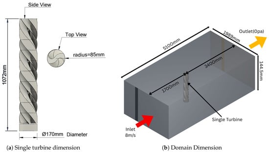
Figure 6.
Images showing (a) dimension of the single turbine, (b) the dimension of the wind tunnel, and inlet and outlet (0 Pa) boundary conditions for testing the single turbine.

Table 1.
Boundary conditions of the simulated model domain.
For the single-turbine simulations, which were conducted to identify the optimal helix angle, the computational domain was defined as follows (with turbine diameter ):
- Inlet is located at a distance of upstream of the turbine;
- Outlet located at a distance of downstream;
- Domain height of ;
- Domain width of .
To evaluate the turbine performance, the torque coefficient () was used as a key parameter. The torque coefficient is defined as follows [12,36]:
where
- T = torque acting on the turbine (Nm);
- = density of air (kg/m3);
- A = frontal area of the turbine (m2);
- R = radius of the turbine (m);
- V = incoming velocity of air (m/s).
The torque coefficient provides a dimensionless representation of the turbine performance, allowing results to be normalized and compared across varying conditions. Torque (T) is directly related to through the above relation, meaning that higher torque values correspond to higher torque coefficients for given flow conditions.
3.3. Simulation Details for Finding the Optimal Distance Between the Blades of the VAWTs
The simulations were again carried out in a three-dimensional wind tunnel domain. Two materials were employed in the model: air as the working fluid and (ABS) plastic as the solid part for the turbine blades. The turbine geometry used in all spacing cases corresponded to the single-turbine geometry described previously (height H = 1.00 m, diameter D = 0.17 m). All boundary conditions were prescribed (0 unknowns). The following solver and boundary settings were used:
- Flow regime: Turbulent, compressible flow (compressible solver option was enabled).
- Turbulence model: Standard k-epsilon.
- Inlet: One velocity inlet with free-stream velocity V = 8 m/s.
- Outlet: One pressure outlet located on the wall opposite the inlet, with gauge pressure set to 0 Pa.
- Room temperature: 33 °C.
- Solver time-marching: 100 steps; each step was run with 1 iteration.
Although compressibility was enabled in the solver, the flow remained in the low-Mach regime (Mach « 0.3), making compressibility effects negligible; however, solver settings were kept consistent across all cases. The global mesh statistics for the model were as follows: total nodes = 994,196 and total elements = 3,966,264. The spacing cases were selected to span a wide range, from closely coupled to weakly interacting configurations, with inter-turbine edge-to-edge spacings of 0 cm, 0.5 cm, 1.66 cm, 4 cm, 7 cm, 11 cm, and 16 cm. Corresponding non-dimensional spacings, normalized using the rotor diameter (D = 17), were Sp/D = [0, 0.029, 0.094, 0.23, 0.41, 0.64, 0.94]. Presenting spacing non-dimensionally allows the results to be generalized across different rotor sizes.
As shown in Figure 7 and Table 2, all lateral tunnel walls that were perpendicular to the inlet–outlet direction (top, bottom, and side walls) were modeled as slip surfaces so that boundary layer formation on those walls was suppressed and artificial wall effects were minimized. The front (inlet) and back (outlet) faces of the tunnel were prescribed as the velocity inlet and the pressure outlet, respectively. The rotor surfaces were treated as non-slip ABS solid surfaces, with the appropriate material properties being assigned for force/torque extraction.
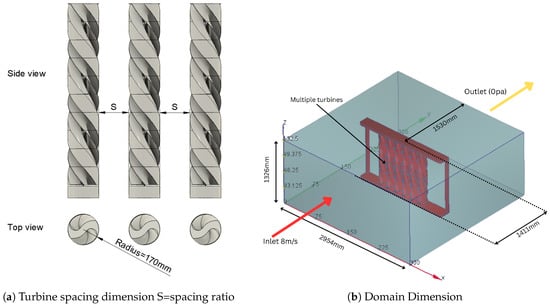
Figure 7.
Images showing (a) dimension of the spacing of turbines, (b) dimension of the wind tunnel, and inlet and outlet (0 Pa) boundary conditions for testing of multiple turbines.
Table 2.
Boundary conditions of the simulated model domain.
For the multiple-turbine simulations, which were performed to evaluate inter-turbine spacing effects, the domain dimensions were as follows:
- Inlet located at upstream;
- Outlet located at downstream;
- Domain height of ;
- Domain width of .
4. Grid Independence Test
A grid independence test for this study was conducted, employing the maximum spacing ratio of 16 and a helix angle of 60 degrees, to ascertain the optimal mesh size required for our computational analysis. A series of mesh configurations ranging from 0.2 to 0.5 million cells were developed and assessed. Table 3 presents a comprehensive summary of the torque and moment coefficients calculated for each mesh size. The data indicates that the mesh labeled as , comprising 3,966,264 cells, exhibits the least relative error, rendering it the most suitable mesh size for subsequent simulations.
Table 3.
Grid independence test: torque and coefficient of moment (Cm) for helix angle of 60 and spacing ratio of 16. The color highlight is for showing that is the best suited Mesh size.
A typical mesh used for the three-blade VAWT configuration is shown in Figure 8.
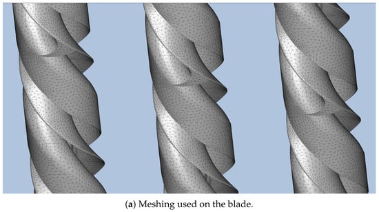
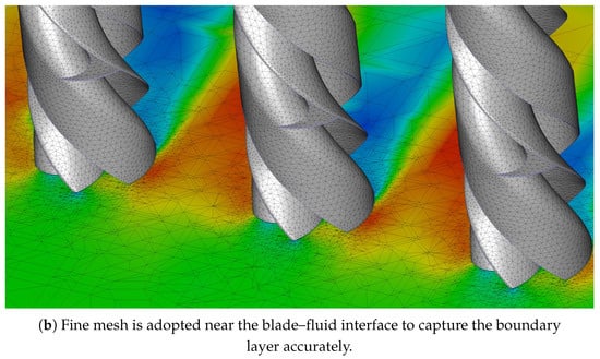
Figure 8.
A typical mesh used for the 3-blade VAWT configuration.
5. Error Analysis and Uncertainty
A comprehensive error and uncertainty analysis was done to ensure the reliability of the CFD predictions. Spatial discretization uncertainty was quantified using a six-level grid refinement study and the Grid Convergence Index (GCI). The fine-grid GCI for the key output variable was found to be 3%, indicating that the numerical solution is grid-independent. Iterative uncertainty was minimized by reducing residuals below and verifying that monitored quantities changed by less than 0.2% with additional iterations. Turbulence model uncertainty was evaluated by comparing the baseline k– model with the k– SST model, resulting in a variation of 7%. Boundary condition sensitivity tests (±10% inlet turbulence intensity) led to variations of 3%. The values along walls were maintained within 30–100, consistent with wall function requirements. The combined CFD uncertainty, calculated using the root-sum-square method, is estimated at ±8.2%. This uncertainty level is acceptable for engineering design and consistent with values reported in the literature.
6. Validation of the Numerical Algorithm
To make sure that the correctness and reliability of the numerical model employed in this research is reliable, we utilized the experimental data provided by McLaren [44], as well as the findings of Divakar et al. [31]. In the experimental investigations, a vertical-axis wind turbine (VAWT) with a 420 mm chord and three blades arranged in a straight configuration was examined and subjected to wind tunnel testing. Similarly, Divakar et al. [31] conducted their numerical analysis with equivalent dimensional parameters and under the same conditions. In this work, we replicated this scenario using our current computational code, maintaining identical boundary and initial conditions to those applied in the referenced studies. Figure 9 presents a comparative analysis of the outcomes achieved through our numerical scheme with McLaren’s experimental results and the computational findings from Divakar et al. This comparison distinctly illustrates the substantial concordance between our numerical code and the pre-existing methodologies, with observed discrepancies not exceeding 5%. Such findings provide a robust foundation of confidence in the numerical model configurations adopted for this study, underscoring their validity and applicability to the problem at hand.
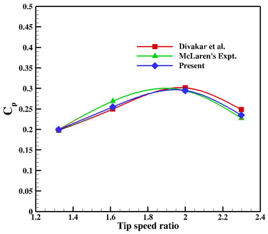
Figure 9.
Validation: Comparison of the results obtained from the present simulation with McLaren’s experimental data [44] and Divakar et al. [31].
7. Results and Discussions
Comprehensive simulations were performed using the software ‘Autodesk CFD’ (version 2024) to thoroughly investigate the impact of varying the helix angle and the spacing ratio on the aerodynamic efficiency of the proposed blade design. The input values for these parameters are listed in Table 4. The evaluation of the blade’s capabilities was conducted using specific performance metrics, namely the torque generation and the moment coefficient associated with the blade, to provide a detailed understanding of its performance characteristics. The subsequent sections provide an in-depth examination and discussion of these various aspects.
Table 4.
The input values for spacing between the blades and the helix angles used.
7.1. Effect of the Helix Angle on the Torque and Moment Coefficient
Table 5 presents the variation in torque and moment coefficient (Cm) with the helix angle. Each case corresponds to a specific twist angle of the turbine blade, with the resulting torque (in Nm) and corresponding Cm values being listed. It can be observed that torque and Cm increase significantly from (0°) by 471% at just 20° of helical twist, reaching peak values at 50–60°(around 831%), (both with reference to 0°). In contrast, the untwisted case (0°) shows minimal performance, highlighting the importance of blade twist in enhancing turbine efficiency to a substantial degree.
Table 5.
Variation in torque and coefficient of moment (Cm) for different helix angles.
From the simulations, it was observed (form Figure 10) that the introduction of a slight helical twist (approximately 10°, and below 20°) increased the torque produced by the turbine to nearly twice that of a turbine without any twist [37,45]. Further increases in the twist angle (beyond 20°) resulted in torque values that were up to five times higher than those of the untwisted configuration [34]. Between 20° and 40°, the increase in torque became less pronounced, with values stabilizing around a near-optimum range [46]. At approximately 50°, a further rise in torque was noted, although subsequent increases in twist produced only marginal improvements. The simulations were limited to a maximum twist of 60° due to the increasing complexity associated with modeling and manufacturing highly twisted blades. In practice, fabricating a turbine with a Ugrinsky profile and high helical twist presents significant design and cost challenges [12].
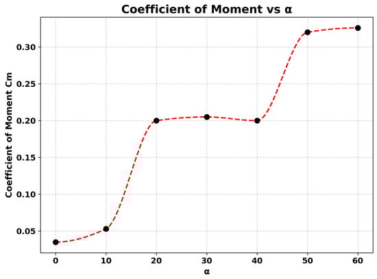
Figure 10.
Variation in coefficient of moment with change in helix angle.
The results can also be stated in terms of the coefficient of moment (Cm). A similar trend was observed, where Cm increased sharply at lower twist angles, nearly doubling at 10° (from 0.035 to 0.053) and reaching up to five times the untwisted value between 20° and 30° (from 0.035 to 0.2) [37,45]. Beyond this range, the growth in Cm began to plateau, showing only incremental improvements until approximately 50° [34]. At this point, a secondary increase was observed (from 0.2 to 0.32), after which further twisting produced negligible gains. This curve indicates that the aerodynamical performance of the turbine is highly sensitive to small twists at low angles but becomes less responsive at higher twists, as the blades begin to shed or deflect airflow rather than capturing it efficiently [46].
The analysis indicates that an optimum helix angle for the Wind Wall lies within the range of 20–30° [37,45]. In this range, the torque output and coefficient of moment are significantly improved compared to the 0-degree helix case, while the structural design and manufacturing process remain manageable. Although higher angles (50–60°) demonstrated higher torque coefficients, the added benefit is offset by the greater complexity and expense of blade fabrication in real applications [12]. From a practical perspective, an increase in the coefficient of moment alone does not justify the higher production costs, as the primary goal is to maximize the net energy output while maintaining economic feasibility.
Figure 11 illustrates static pressure contours and velocity vectors at the turbine’s midplane, perpendicular to its axis, for three different helix angles: 0, 20, and 40 degrees. The contours indicate a continuous rise in front stagnation pressure as the helix angle increases from 0 to 40 degrees. Similarly, the negative pressure region behind the blade increases, and the chaotic nature of the wake intensifies (observed from velocity vectors) with a greater helix angle. The pressure differential between the turbine’s front and back generates torque and on the blade, which escalates with the helix angle.
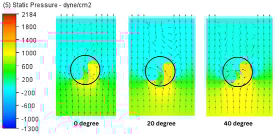
Figure 11.
Static pressure contours and velocity vectors plotted at the midplane of the turbine perpendicular to its axis for different turbine helical twists. The black circles represent the surface of the turbine.
The turbine’s performance assessment traditionally relies on the torque and moment coefficient (). However, the drag force is another significant parameter impacting the performance of the turbine, attributed to flow separation that is induced by adverse pressure gradients on the turbine’s surface. This creates a trade-off between these factors and the drag force. As shown in Figure 11 of this manuscript, increased helix angles lead to adverse pressure gradients, prompting premature flow separation and heightened drag. Hence, evaluating turbine performance purely through torque or is insufficient without considering drag. We introduce two parameters, T/ and /, providing a more comprehensive performance metric, where T denotes the generated torque and is the drag coefficient. Figure 12 illustrates torque, , T/, and / variations with the helix angle, highlighting enhanced performance at 20-30 degrees, with subsequent declines due to rising . Therefore, the optimum helix angle is defined not only by aerodynamic performance but by a balance between torque enhancement, coefficient of moment behavior, drag behaviour, manufacturability, and cost-effectiveness [34,37,45]. This trade-off ensures that the Wind Wall remains both technically efficient and economically feasible, thus fulfilling its purpose of delivering reliable electricity generation in a scalable and practical form.
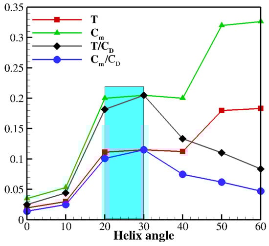
Figure 12.
Variation in torque (T), , T/, and / with helix angle. The performance parameters T/ and / show better performance in the range of 20–30 degrees for the helix angle.
7.2. Effect of Spacing Between the Blades on the Torque and Moment Coefficient
The spacing between turbine blades plays an important role in aerodynamic performance of the blades. This section delves into a detailed analysis of how variations in blade spacing influence both the torque and the coefficient of moment (Cm) across a range of helix angles associated with the blades. By examining these dynamics, the study aims to elucidate the complex interplay between blade arrangement and overall turbine performance, thus providing deeper insights into the aerodynamic optimization of turbine systems.
Figure 13 represents contours of velocity magnitude and velocity vectors at the turbine’s midplane, perpendicular to its axis, for three different gaps, 0.5 cm, 7 cm, and 16 cm, which will substantiate the physical interpretation of the acceleration mechanisms occurring between closely spaced turbines. These visualizations clearly show a progressive trend: when the turbines are placed very close to each other—almost at zero spacing—the airflow between them is heavily restricted, causing the inter-turbine velocity to remain low. As the spacing gradually increases toward the optimum value, the flow is able to accelerate more freely, resulting in a noticeable increase in air velocity between the turbines.
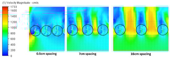
Figure 13.
Contours of magnitude of velocity and velocity vectors, plotted at the midplane of the turbine perpendicular to its axis for different turbine helical twists. The black circles represent the surface of the turbine.
However, once the spacing goes beyond this optimum point, the beneficial interaction between the turbines diminishes. The accelerated flow effect weakens, and the inter-turbine velocity begins to decline. Eventually, at sufficiently large spacings, the airflow between the turbines behaves almost as if the turbines were isolated, and the velocity returns to roughly the same value as the incoming free-stream wind.
- Optimal spacing for 0-degree helix turbines:The results as show in in Table 6 and Figure 14 for the 0-degree helix configuration show a clear dependence of the coefficient of moment (Cm) on the spacing between adjacent turbines. At zero spacing, the torque and Cm values are relatively low (T = 0.052 Nm, Cm = 0.092) due to strong wake interference. As the spacing increases slightly to 0.5–1.6 cm, both the torque and Cm increase significantly, reaching Cm = 0.158. The maximum performance is observed at a spacing of 4 cm (Cm = 0.22), where constructive flow acceleration through the narrowed passage appears to enhance the effective velocity on the turbine. Beyond this optimum spacing, a rapid decline in performance is observed, with Cm dropping back to near baseline levels at 7 cm (0.096) and further diminishing to very low values at 11–16 cm (0.027).
Table 6. Variation in torque and coefficient of moment (Cm) for different spacings at helix angle of 0°.
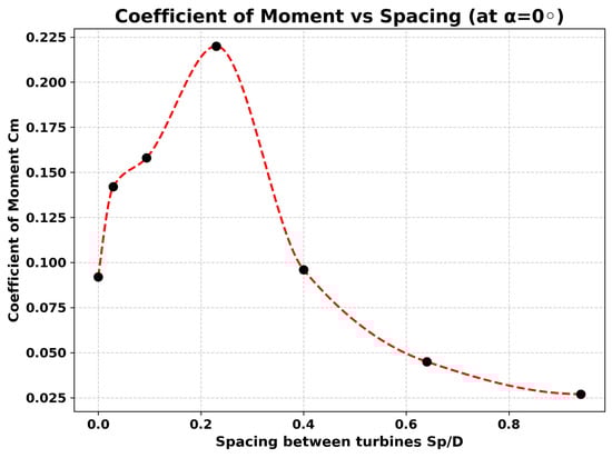 Figure 14. Variation in coefficient of moment with change in distance between the turbines ().
 - Optimal spacing for 10 degrees helix turbines:For the 10-degree helix configuration as show in in Table 7 and Figure 15, the variation in torque and coefficient of moment (Cm) with turbine spacing demonstrates a distinct performance profile. At zero spacing, the initial Cm is slightly higher than the 0° case (Cm = 0.107), reflecting the stabilizing effect of the helical twist in reducing destructive interference. A gradual increase is observed at a spacing of 0.5 cm (Cm = 0.119), followed by a sharp rise to the peak value of Cm = 0.217 at 1.6 cm. This indicates that the helical twist enables stronger constructive aerodynamic interactions at relatively closer spacings than in the untwisted configuration, likely due to smoother flow redirection and reduced pulsations in the torque.
Table 7. Variation in torque and coefficient of moment (Cm) for different distances at helix angle of 10°.
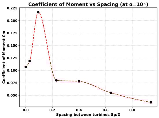 Figure 15. Variation in coefficient of moment with change in distance between the turbines ().
 - Optimal spacing for 20-degree helix turbines:This results as show in in Table 8 and Figure 16 shows us that the turbine interaction is highly spacing-dependent, with maximum aerodynamic benefit occurring at smaller separations. Starting from a baseline Cm = 0.092 at zero spacing, performance rises sharply to a peak of Cm = 0.35 (torque 0.196 Nm) at 1.6 cm, nearly quadrupling the baseline due to strong constructive flow interactions and a Venturi-like effect that boosts the effective velocity. Beyond this optimum range (0.5–1.6 cm), the moment coefficient declines rapidly, dropping to 0.1 by 11 cm, although a minor recovery to 0.138 at 16 cm suggests residual flow re-alignment. Overall, these findings highlight that close turbine spacing strongly enhances aerodynamic performance, while larger spacings diminish interactions and cause the turbines to behave more independently.
Table 8. Variation in torque and coefficient of moment (Cm) for different distances at helix angle of 20°.
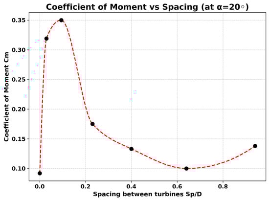 Figure 16. Variation in coefficient of moment with change in distance between the turbines ().
 - Optimal spacing for 30-degree helix turbines:In this scenario as show in in Table 9 and Figure 17, the turbine’s performance shows a more gradual and sustained enhancement compared to the previous case. Starting from a baseline of Cm = 0.151 at zero spacing, the coefficient increases steadily with separation, peaking at Cm = 0.215 (torque 0.115 Nm) at 7 cm. Unlike the sharp optimum observed earlier, this setup exhibits a broader effective range, with relatively high values being maintained between 4 and 7 cm before declining moderately at larger spacings (Cm = 0.18 at 11 cm and 0.17 at 16 cm). This trend suggests that the aerodynamic interaction is less dependent on very close spacing and instead benefits from a wider spacing window, where flow stabilization and smoother energy exchange between turbines sustain improved performance due to the change in the helix angle.
Table 9. Variation in torque and coefficient of moment (Cm) for different distances at helix angle of 30°.
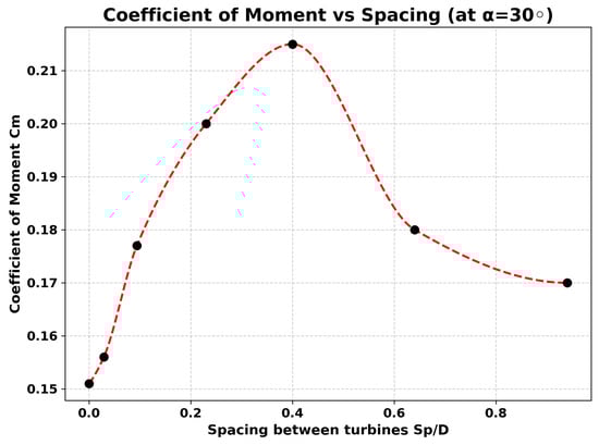 Figure 17. Variation in coefficient of moment with change in distance between the turbines ().
 - Optimal spacing for 40-degree helix turbines:In this case as show in in Table 10 and Figure 18, turbine interaction peaks at a very small spacing before rapidly diminishing. The baseline performance at zero spacing is already strong (Cm = 0.197), rising slightly to its maximum of Cm = 0.218 (torque 0.122 Nm) at 0.5 cm. However, unlike previous configurations, the performance drops sharply at 1.6 cm (Cm = 0.144) and only partially recovers at 4–11 cm, where values stabilize around Cm = 0.171–0.172. At the largest spacing of 16 cm, the coefficient decreases further to 0.14. Furthermore, for this helix angle, there is a plateauing effect of the Cm from a distance coefficient of 0.2–0.638 and then a further decrease.
Table 10. Variation in torque and coefficient of moment (Cm) for different distances at helix angle of 40°.
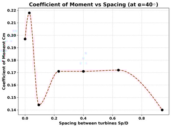 Figure 18. Variation in coefficient of moment with change in distance between the turbines ().
 - Optimal spacing for 50-degree helix turbines:At 50 degrees as show in in Table 11 and Figure 19, the turbine displays a distinctive interaction pattern with both strong initial performance and an unusually late surge. At zero spacing, the turbines already achieve a high Cm = 0.257, which remains nearly unchanged at 0.5 cm before gradually declining to 0.21 at 1.6 cm. A partial recovery occurs at 4 cm (Cm = 0.242), followed by another dip at 7 cm. Interestingly, performance rises again at 11 cm (Cm = 0.22) and then shows an anomalously high spike at 16 cm, where Cm jumps to 0.358 despite a very low torque value (0.02 Nm). This suggests that while the turbines maintain relatively strong interactions across small-to-moderate spacings, the unexpected efficiency spike at a large separation may indicate unique flow reorganization or measurement sensitivity at extreme spacings.
Table 11. Variation in torque and coefficient of moment (Cm) for different distances at helix angle of 50°.
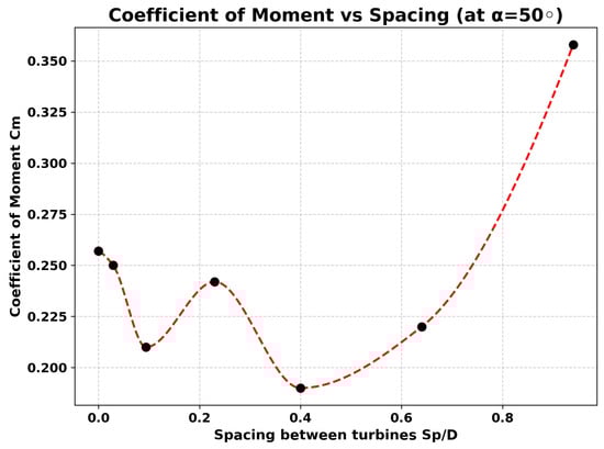 Figure 19. Variation in coefficient of moment with change in distance between the turbines ().
 - Optimal spacing for 60-degree helix turbines:At 60 degrees as show in in Table 12 and Figure 20, the turbines show relatively stable and moderate spacing sensitivity: the baseline at zero spacing is Cm = 0.206 (torque 0.115 Nm), and values only fluctuate mildly with separation, rising slightly to a local peak of Cm = 0.216 (torque 0.121 Nm) at 4 cm and reaching the overall maximum Cm = 0.239 (torque 0.134 Nm) at 11 cm. Intermediate spacings (0.5–7 cm) produce nearly constant performance, with Cm around 0.20–0.213, while the largest spacing (16 cm) shows a modest drop to Cm = 0.189. Overall, this configuration suggests more robust, less spacing-sensitive aerodynamic coupling compared with earlier cases, with a clear mid-to-large spacing optimum near 11 cm.
Table 12. Variation in torque and coefficient of moment (Cm) for different distances at helix angle of 60°.
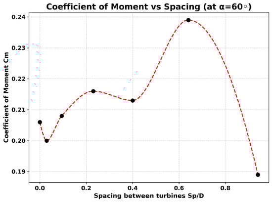 Figure 20. Variation in coefficient of moment with change in distance between the turbines ().
Analysis of Results
The experimental results demonstrate that the inter-turbine spacing and helix angle jointly govern aerodynamic coupling between adjacent VAWT units. Normalizing spacing by rotor diameter (s = spacing/D) reveals that some helix angles produce strong, narrow peaks in the moment coefficient at small s (e.g., 10 degrees and 20 degrees at s = 0.094), while other angles (30 degrees and 60 degrees) show broader mid-spacing optima (s = 0.412–0.647). As in the Figure 21 we can interpret sharp small-spacing maxima as the result of local flow acceleration through a constricted passage, combined with constructive phase alignment of shed vortical structures that augment blade loading. In contrast, larger helix angles introduce axial flow components and smoother temporal loading, giving more performance over a wider spacing window. It is seen that at higher helix angles, the maximum of Cm is reached at a larger spacing between the turbines. Taken together, these results indicate a trade-off between the peak achievable moment coefficient and spacing tolerance: angles that produce very large peaks are highly sensitive to spacing, whereas angles with modest maxima but broad plateaus (30 degrees–60 degrees) are preferable for practical, mass-produced Wind Wall installations if the complexity of manufacturing a highly twisted blade can be reduced.
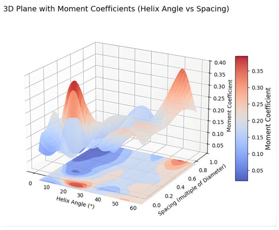
Figure 21.
Three-dimensional plot showing various moment coefficients for different helix angles at different spacings.
7.3. Correlation Between the Effective Velocity and Distance Coefficient
In a Wind Wall configuration, the VAWTs are positioned in series, which causes the incoming wind to undergo a Venturi effect due to the presence of adjacent turbines. This aerodynamic phenomenon accelerates the airflow between the turbines, thereby increasing the effective velocity () experienced by each turbine [19,31,32]. As a result, the torque that is generated on the turbine blades rises significantly.
The torque (T) on a turbine can be expressed as follows [12,36]:
A simplified inverse-spacing model is often used to describe the acceleration between closely spaced rotors:
where is the non-dimensional spacing, and characterizes the aerodynamic interaction strength [19,31]. While this form captures the qualitative increase in at small S values, it cannot reproduce the non-monotonic behavior observed in turbine arrays.
However, the CFD results of the present study show that the relationship between and S is non-monotonic, with a clear peak occurring at a moderate spacing (–). This makes the expression unsuitable for quantitative prediction. To obtain a physically consistent and dimensionally correct relationship, a multiplicative exponential interaction model was adopted:
where c, a, b, and n are dimensionless parameters obtained from nonlinear least-squares fitting of the CFD data. For the present turbine geometry and helix angle, the fitted values are as follows:
This form reproduces the peak in , matches the observed CFD trend with high accuracy (RMSE = 0.1367), and satisfies the correct physical limit as , reflecting the blockage-dominated region at very small spacings.
The trend predicted by the improved correlation is consistent with observations reported in the literature. Dabiri [19] and Jodai & Hara [25,26] reported Venturi-induced flow acceleration between closely spaced VAWTs, while numerical studies [27,47] observed spacing-dependent peaks in inter-turbine velocity. Although the present work evaluates blade spacing effects arising from helical geometry rather than inter-turbine spacing, the underlying aerodynamic mechanisms are analogous, and the predicted spacing range aligns well with these studies.
For the present study, the incoming wind speed (V) is fixed at 8 m/s. Using the above correlation and CFD-derived parameters, the optimal spacing can be determined to maximize the effective velocity and, consequently, the torque generation of the Wind Wall system.
The relationship between Ve, Ve from correlation, and S is shown in the graph below (Figure 22).
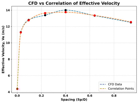
Figure 22.
Graph showing the effective velocity(Ve) for different turbine spacings.
8. Conclusions
The present work employed Computational Fluid Dynamics to investigate the aerodynamic behavior of a vertical-axis wind turbine (VAWT) system based on a symmetrical Ugrinsky blade profile. Using Autodesk CFD, the study focused on determining the optimal helix angle–spacing combinations and establishing a correlation between effective velocity and blade spacing. The results demonstrate that integrating helical twists and appropriate spacing configurations can significantly enhance torque generation and broaden the design flexibility of Wind Wall systems.
8.1. Findings and Observations
- Helix angle optimization: A moderate helix angle (10–30°) improves torque uniformity and reduces pulsations, with an angle of approximately 20° being identified as the most practical balance between aerodynamic efficiency and manufacturability.
- Effect of larger twists: Larger helix angles can yield additional torque gains, but the associated fabrication complexities increase disproportionately, limiting their feasibility for real-world use.
- Influence of blade spacing: Inter-blade spacing strongly affects turbine performance due to Venturi-like flow acceleration between blades. Appropriate spacing enhances the effective velocity and, consequently, the torque output.
- Velocity–spacing correlation: A predictive relationship between effective velocity and spacing has been established, enabling more efficient Wind Wall design without relying solely on iterative trial-based configurations.
- Advantages of Ugrinsky blades: The combination of Ugrinsky-profile blades and a helical twist improves energy capture at low wind speeds and enhances adaptability to varying wind directions.
- Application potential: The Wind Wall configuration is well-suited for compact or constrained environments such as beach boardwalks, airport boundaries, rooftop installations, inter-building corridors, and coastal promenades where wind funneling naturally enhances flow.
- Alignment with the literature: The trends observed in this study agree with established experimental and numerical findings reported in prior works [19,28,29,31,32].
- Structural and Deployment Considerations: Beyond aerodynamic optimization, practical deployment of the Wind Wall requires evaluation of structural robustness, material selection, and manufacturability. Turbines that are subjected to fluctuating aerodynamic loads necessitate fatigue-resistant materials and joints, while the support frames must withstand both static and dynamic stresses originating from wind-induced oscillations. Lightweight alloys, fiber-reinforced polymers, or modular steel assemblies offer favorable strength–weight trade-offs for large-scale implementation. Manufacturing factors such as blade forming tolerances, twist accuracy, and assembly repeatability also influence performance consistency. Furthermore, real-world deployment demands modular installation strategies, maintainability, and cost-efficient scaling, enabling the Wind Wall to function reliably in diverse and harsh environments.
8.2. Future Research Directions
- Investigate the aerodynamic and structural implications of larger helix angles beyond the moderate range.
- Conduct dynamic and transient simulations under variable wind conditions to capture unsteady effects.
- Employ multivariable optimization to identify interaction effects between helix angle and inter-turbine spacing.
- Extend the proposed velocity–spacing correlation using larger datasets and experimental validation to improve generality and predictive capability.
- Evaluate long-term performance, fatigue behaviour, and the scalability of the Wind Wall concept for real-world deployment.
Author Contributions
Conceptualization, P.L. and A.K.S.; methodology, P.L. and A.K.S.; software, P.L.; validation, P.L. and A.K.S.; formal analysis, P.L.; investigation, P.L., S.M. and A.K.S.; resources, P.L. and A.K.S.; data curation, P.L.; writing—original draft preparation, P.L.; writing—review and editing, P.L., S.M. and A.K.S.; visualization, P.L.; supervision, S.M. and A.K.S.; project administration, S.M. and A.K.S.; funding acquisition, S.M. and A.K.S. All authors have read and agreed to the published version of the manuscript.
Funding
This research received no external funding.
Data Availability Statement
The original contributions presented in this study are included in the article. Further inquiries can be directed to the corresponding authors.
Conflicts of Interest
The authors declare no conflicts of interest. The funders had no role in the design of the study; in the collection, analyses, or interpretation of data; in the writing of the manuscript; or in the decision to publish the results.
Nomenclature
| Latin Symbols | |
| A | Frontal area of turbine (m2) |
| Moment coefficient | |
| D | Turbine diameter (m) |
| H | Turbine height (m) |
| Aerodynamic interaction coefficient | |
| R | Turbine radius (m) |
| S | Spacing ratio () |
| Edge-to-edge turbine spacing (m) | |
| T | Torque acting on turbine (N·m) |
| Velocity component in direction j (m/s) | |
| V | Free-stream velocity (m/s) |
| Effective velocity between turbines (m/s) | |
| Greek Symbols | |
| Density of air (kg/m3) | |
| Dynamic viscosity (Pa·s) | |
| Turbulent eddy viscosity (Pa·s) | |
| Turbulent dissipation rate (m2/s3) | |
| k | Turbulent kinetic energy (m2/s2) |
| Helix angle (°) | |
| Subscripts | |
| e | Effective value |
| ∞ | Free-stream or far-field value |
References
- Boyle, G. Renewable Energy: Power for a Sustainable Future, 3rd ed.; Oxford University Press: Oxford, UK, 2012. [Google Scholar]
- Murali, D.; Ajith Kumar, R.; Ajith Kumar, S. On the laminar wake of curved plates. Phys. Fluids 2024, 36, 4. [Google Scholar] [CrossRef]
- Smil, V. Energy and Civilization: A History; MIT Press: Cambridge, MA, USA, 2017. [Google Scholar]
- Smil, V. Energy Transitions: History, Requirements, Prospects; Praeger: Santa Barbara, CA, USA, 2010. [Google Scholar]
- Fouquet, R. The slow search for solutions: Lessons from historical energy transitions by sector and service. Energy Policy 2010, 38, 6586–6596. [Google Scholar] [CrossRef]
- Grübler, A. Transitions in energy use. In Encyclopedia of Energy; Cleveland, C.J., Ed.; Elsevier: Amsterdam, The Netherlands, 2004; Volume 6, pp. 163–177. [Google Scholar]
- Perkins, J.H. Energy Transitions: Linking Energy and Climate Change; Springer Nature: Cham, Switzerland, 2019; pp. 87–106. [Google Scholar] [CrossRef]
- Connor, M.; Berners-Lee, M.; Davies, M.; Gilbert, P.; Saklar, N. Effects of fossil fuel and total anthropogenic emission removal on public health and climate. Proc. Natl. Acad. Sci. USA 2019, 116, 7192–7197. [Google Scholar]
- Smith, J.; Lee, E.; Martinez, C. Air pollution from fossil fuel use accounts for over 5 million excess deaths per year globally. Br. Med J. (BMJ) 2024, 380, e072567. [Google Scholar]
- Manwell, J.F.; McGowan, J.G.; Rogers, A.L. Wind Energy Explained: Theory, Design and Application, 2nd ed.; John Wiley & Sons: Hoboken, NJ, USA, 2010. [Google Scholar]
- Burton, T.; Jenkins, N.; Sharpe, D.; Bossanyi, E. Wind Energy Handbook, 2nd ed.; John Wiley & Sons: Hoboken, NJ, USA, 2011. [Google Scholar]
- Paraschivoiu, I. Wind Turbine Design: With Emphasis on Darrieus Concept; Polytechnic International Press: Hong Kong, China, 2002. [Google Scholar]
- Rott, A.; Schmidt, M.; Marten, D.; Peinke, J.; Hölling, M. Wind vane correction during yaw misalignment for horizontal-axis wind turbines. Wind Energy Sci. 2023, 8, 1755–1768. [Google Scholar] [CrossRef]
- Mittelmeier, N.; Kühn, M. Determination of Optimal Wind Turbine Alignment with SCADA Data. Wind Energy Sci. 2018, 3, 395–408. [Google Scholar] [CrossRef]
- AIS Wind Energy. Advantages and Disadvantages of Horizontal Axis and Vertical Axis Wind Turbines, 2023. Available online: https://aiswindenergy.co.uk/advantages-and-disadvantages-of-horizontal-axis-and-vertical-axis-wind-turbines/ (accessed on 8 June 2025).
- Ajith Kumar, S.; Anil Lal, S. Effects of Prandtl Number on Three Dimensional Coherent Structures in the Wake behind a Heated Cylinder. J. Appl. Fluid Mech. 2020, 14, 515–526. [Google Scholar] [CrossRef]
- Saidur, R.; Rahim, N.A.; Islam, M.R.; Solangi, K.H. Environmental impact of wind energy. Renew. Sustain. Energy Rev. 2011, 15, 2423–2430. [Google Scholar] [CrossRef]
- Leung, D.Y.C.; Yang, Y. Wind energy development and its environmental impact: A review. Renew. Sustain. Energy Rev. 2012, 16, 1031–1039. [Google Scholar] [CrossRef]
- Dabiri, J.O. Potential Order-of-Magnitude Enhancement of Wind Farm Power Density via Counter-Rotating Vertical-Axis Wind Turbine Arrays. J. Renew. Sustain. Energy 2011, 3, 043104. [Google Scholar] [CrossRef]
- Zamre, P.; Lutz, T. Computational-fluid-dynamics analysis of a Darrieus vertical-axis wind turbine installation on the rooftop of buildings under turbulent-inflow conditions. Wind Energy Sci. 2022, 7, 1661–1680. [Google Scholar] [CrossRef]
- Srinivasan, L.; Ram, N.; Rengarajan, S.B.; Divakaran, U.; Mohammad, A.; Velamati, R.K. Effect of Macroscopic Turbulent Gust on the Aerodynamic Performance of Vertical Axis Wind Turbine. Energies 2023, 16, 2250. [Google Scholar] [CrossRef]
- U.S. Department of Energy. Vertical-Axis Wind Turbines: Applications, Advantages, and Urban Performance, 2023. Search|Department of Energy. Available online: https://www.energy.gov/search?keywords=vertical+axis+wind+turbines&page=0 (accessed on 21 August 2025).
- Hezaveh, S.H.; Bou-Zeid, E.; Dabiri, J.; Kinzel, M.; Cortina, G.; Martinelli, L. Increasing the Power Production of Vertical-Axis Wind-Turbine Farms Using Synergistic Clustering. Bound.-Layer Meteorol. 2018, 169, 275–296. [Google Scholar] [CrossRef]
- Whittlesey, R.W.; Liska, S.; Dabiri, J.O. Fish schooling as a basis for vertical axis wind turbine farm design. arXiv 2010, arXiv:1002.2250. [Google Scholar] [CrossRef]
- Jodai, Y.; Hara, Y. Wind Tunnel Experiments on Interaction between Two Closely Spaced Vertical-Axis Wind Turbines in Side-by-Side Arrangement. Energies 2021, 14, 7874. [Google Scholar] [CrossRef]
- Jodai, Y.; Hara, Y. Wind-Tunnel Experiments on the Interactions among a Pair/Trio of Closely Spaced Vertical-Axis Wind Turbines. Energies 2023, 16, 1088. [Google Scholar] [CrossRef]
- Malge, A.U. Effect of inter turbine spacing in omnidirectional wind for Vertical Axis Wind Turbines. Civ. Eng. (OUP J.) 2025, 9, 94. [Google Scholar] [CrossRef]
- Shahriar, E.; Sagar, M.M.; Alam, M.R.; Rahman, K.A. Design and Fabrication of a Helical Vertical Axis Wind Turbine for Electricity Supply. World J. Adv. Eng. Technol. Sci. 2024, 12, 201–217. [Google Scholar] [CrossRef]
- Sakamoto, L.; Fukui, T.; Morinishi, K. Numerical Study on the Performance of 2-D Ugrinsky Wind Turbine Model. In WIT Transactions on Ecology and the Environment; WIT Press: Southampton, UK, 2021; Volume 254, pp. 113–124. [Google Scholar] [CrossRef]
- Sakamoto, L.; Fukui, T.; Morinishi, K. Blade Dimension Optimization and Performance Analysis of the 2-D Ugrinsky Wind Turbine. Energies 2022, 15, 2478. [Google Scholar] [CrossRef]
- Unnikrishnan, D.; Ajith, R.; Mohammad, A.; Velamati, R.K. Effect of Helix Angle on the Performance of Helical Vertical Axis Wind Turbines. Energies 2021, 14, 393. [Google Scholar] [CrossRef]
- Qin, R.; Duan, C. The Principle and Applications of Bernoulli Equation. In Proceedings of the Journal of Physics: Conference Series, International Conference on Fluid Mechanics and Industrial Applications (FMIA 2017), Taiyuan, China, 21–22 October 2017; Volume 916, p. 012038. [Google Scholar] [CrossRef]
- Biswal, P.; Singh, K.; Ahmed, S.; Saha, U.K. A Review of Augmentation Methods to Enhance the Performance of Vertical Axis Wind Turbine. Sustain. Energy Technol. Assess. 2022, 53, 102469. [Google Scholar] [CrossRef]
- Islam, M.; Ting, D.S.K.; Fartaj, A. Aerodynamic Models for Darrieus-Type Straight-Bladed Vertical Axis Wind Turbines. Renew. Sustain. Energy Rev. 2008, 12, 1087–1109. [Google Scholar] [CrossRef]
- Howell, R.; Qin, N.; Edwards, J.; Durrani, N. Wind Tunnel and Numerical Study of a Small Vertical Axis Wind Turbine. Renew. Energy 2010, 35, 412–422. [Google Scholar] [CrossRef]
- Munson, B.R.; Young, D.F.; Okiishi, T.H. Fundamentals of Fluid Mechanics, 7th ed.; Wiley: Hoboken, NJ, USA, 2013. [Google Scholar]
- Bhutta, M.M.A.; Hayat, N.; Farooq, A.U.; Ali, Z.; Jamil, S.R.; Hussain, Z. Vertical Axis Wind Turbine—A Review of Various Configurations and Design Techniques. Renew. Sustain. Energy Rev. 2012, 16, 1926–1939. [Google Scholar] [CrossRef]
- Castelli, M.R.; Englaro, A.; Benini, E. The Darrieus Wind Turbine: Proposal for a New Performance Prediction Model Based on CFD. Energy 2012, 36, 4919–4934. [Google Scholar] [CrossRef]
- Ferziger, J.H.; Peric, M. Computational Methods for Fluid Dynamics, 3rd ed.; Springer: Berlin/Heidelberg, Germany, 2002. [Google Scholar]
- Reyes, R.; Araya, D.B.; Dabiri, J.O. Effects of Spacing and Alignment on the Performance of Vertical-Axis Wind Turbine Arrays. J. Renew. Sustain. Energy 2020, 12, 023301. [Google Scholar] [CrossRef]
- Launder, B.E.; Spalding, D.B. The numerical computation of turbulent flows. Comput. Methods Appl. Mech. Eng. 1974, 3, 269–289. [Google Scholar] [CrossRef]
- Ajith Kumar, S.; Murali, D.; Sethuraman, V.R.P. Flow control using hot splitter plates in the wake of a circular cylinder: A hybrid strategy. Phys. Fluids 2024, 36, 013624. [Google Scholar] [CrossRef]
- Versteeg, H.K.; Malalasekera, W. An Introduction to Computational Fluid Dynamics: The Finite Volume Method, 2nd ed.; Pearson Education Limited: London, UK, 2007. [Google Scholar]
- McLaren, K.W. A Numerical and Experimental Study of Unsteady Loading of High Solidity Vertical Axis Wind Turbines. Ph.D. Thesis, McMaster University, Hamilton, ON, Canada, 2011. [Google Scholar]
- Shankar, V.; Kumar, R. Performance evaluation of helical Savonius vertical axis wind turbine: A review. Renew. Sustain. Energy Rev. 2018, 82, 1350–1361. [Google Scholar]
- Tjiu, W.; Marnoto, T.; Mat, S.; Ruslan, M.H.; Sopian, K. Darrieus vertical axis wind turbine for power generation: Technology review and design considerations. Renew. Sustain. Energy Rev. 2015, 51, 388–401. [Google Scholar]
- Dinesh Kumar Reddy, G.; Verma, M.; De, A. Performance Analysis of Vertical Axis Wind Turbine Clusters: Effect of Inter-Turbine Spacing and Turbine Rotation. arXiv 2023, arXiv:2310.08001. [Google Scholar] [CrossRef]
Disclaimer/Publisher’s Note: The statements, opinions and data contained in all publications are solely those of the individual author(s) and contributor(s) and not of MDPI and/or the editor(s). MDPI and/or the editor(s) disclaim responsibility for any injury to people or property resulting from any ideas, methods, instructions or products referred to in the content. |
© 2025 by the authors. Licensee MDPI, Basel, Switzerland. This article is an open access article distributed under the terms and conditions of the Creative Commons Attribution (CC BY) license (https://creativecommons.org/licenses/by/4.0/).