A New Asymmetric Track Filtering Algorithm Based on TCN-ResGRU-MHA

Abstract

Modern target tracking systems rely on radar as a sensor to detect targets and generate raw track points. These raw track points are affected by the radar’s own noise and the asymmetric non-Gaussian noise resulting from the nonlinear transformation from polar coordinates to Cartesian coordinates. Without effective processing, such data cannot directly support highly reliable situational awareness, early warning decisions, or weapon guidance. Track filtering, as a core component of target tracking, plays an irreplaceable foundational role in achieving real-time, accurate, and stable estimation of moving target states. Traditional deep learning filtering algorithms struggle with capturing long-term dependencies in high-dimensional spaces, often exhibiting high computational complexity, slow response to transient signals, and compromised noise suppression due to their inherent architectural asymmetries. In order to address these issues and balance the model’s high accuracy, strong real-time performance, and robustness, a new trajectory filtering algorithm based on a temporal convolutional network (TCN), Residual Gated Recurrent Unit (ResGRU), and multi-head attention (MHA) is proposed. The TCN-ResGRU-MHA hybrid structure we propose combines the parallel processing advantages and detail-capturing ability of a TCN with the residual learning capability of a ResGRU, and introduces the MHA mechanism to achieve adaptive weighting of high-dimensional features. Using the root mean square error (RMSE) and Euclidean distance to evaluate the model effect, the experimental results show that the RMSE of TCN-ResGRU-MHA is 27.4621 (m) lower than CNN-GRU, which is an improvement of 15.99% in the complex scene of high latitude, and the distance is 37.906 (m) lower than CNN-GRU, which is an improvement of 18.65%. These results demonstrate its effectiveness in filtering and tracking tasks in high-latitude complex scenarios.

1. Introduction

1.1. Background

Modern target tracking systems (such as air defense early warning, air traffic control, missile defense, and autonomous driving perception systems) all rely on radar as the primary long-range, all-weather detection tool [1,2,3,4,5,6,7,8,9]. Radar sensors periodically scan the environment, detect targets, and generate raw track points [10,11,12,13,14,15,16,17]. However, radar track data has the following characteristics: inherent noise and uncertainty, as radar measurements are subject to thermal noise, clutter interference, multipath effects, and other factors, leading to significant random errors in the obtained position and velocity information; limited angular resolution and uneven distance measurement accuracy, meaning that a single measurement cannot reflect the target’s true state; discrete sampling characteristics, as radar operates on a fixed cycle, so the target’s state can only be ‘captured’ at discrete time points; and nonlinear and non-ideal motion, as radar typically measures in polar coordinates, while targets often move in Cartesian coordinates and frequently maneuver. Coordinate transformation introduces nonlinear errors, and the target’s actual motion often deviates from simplified motion models. These issues, dictated by both radar hardware characteristics and the detection environment, result in raw track points naturally containing noise disturbance, data gaps, position jumps, and accuracy limitations. Without effective processing, such data cannot directly support high-reliability situational awareness, early warning decisions, or weapon guidance [18].

To achieve real-time, accurate, and stable estimation of a moving target’s state, track filtering serves as the core component of target tracking, playing an irreplaceable foundational role. Track filtering processes the sequence of sensor detection points through temporal fusion, eliminating noise, compensating for uncertainty, and associating measurements with the true target motion, ultimately generating a smooth, continuous, and reliable target track that can be used to predict future positions [19,20].

1.2. Current Methods Review

The historical development of filtering algorithms has broadly progressed through three distinct phases: Initially dominated by elementary techniques such as moving averages and polynomial fitting, subsequent evolution shifted toward state-space model-based methodologies, culminating in the current era, where machine learning approaches demonstrate significant potential, enabled by advances in computational capabilities. Among conventional methods, the Kalman Filter (KF) [21] gained widespread adoption owing to its optimal estimation properties, though its inherent linearity constraints limit efficacy in nonlinear systems. To address this limitation, researchers developed enhanced variants including the Extended Kalman Filter (EKF) and Unscented Kalman Filter (UKF).

The Extended Kalman Filter (EKF) utilizes local linearization through first-order Taylor expansion to approximate nonlinear system dynamics and observation models, subsequently implementing the standard Kalman filtering framework for state estimation [22]. Primary advantages of this approach include computational efficiency, primarily attributable to the sole requirement of Jacobian matrix computation; effective applicability in real-time operational scenarios; and operational maturity in engineering implementations, with demonstrated stability in weakly nonlinear systems. Nevertheless, fundamental limitations persist: non-negligible linearization errors arising from first-order truncation, inducing systematic state-space distortion; precipitous accuracy deterioration or filter divergence under strongly nonlinear conditions; analytical intractability of Jacobian derivations for complex systems, necessitating error-prone numerical approximations that elevate computational complexity and uncertainty propagation; and heightened sensitivity to initialization inaccuracies and parametric mismatches, potentially inducing catastrophic failure through linearization breakdown.

The Unscented Kalman Filter (UKF) propagates the statistical properties of nonlinear systems through a set of deterministically selected sigma points via the unscented transform (UT), thereby circumventing the linearization process. Core advantages of this methodology include superior estimation accuracy, attributable to full capture of second-order statistical characteristics in nonlinear systems; demonstrated performance advantages over Extended Kalman Filters (EKFs) for high-maneuvering target tracking [23,24]; elimination of Jacobian matrix computations, simplifying implementation and mitigating model-mismatch risks; and enhanced numerical stability with robustness against parametric uncertainties and noise non-stationarity. However, inherent limitations require attention: computational complexity escalation resulting from the 2n + 1 sigma-point requirement, where n denotes state dimension, constraining real-time performance in high-dimensional systems; and inherent Gaussian noise assumption, leading to persistent estimation bias under heavy-tailed distributions within complex electromagnetic environments.

The Particle Filter (PF) algorithm approximates the posterior probability distribution through large-scale Monte Carlo simulations with weighted particles. While effectively addressing nonlinear and non-Gaussian system constraints, this methodology exhibits three fundamental limitations: excessive computational load inherent to particle propagation mechanisms; progressive particle degeneracy requiring systematic resampling interventions; compromised real-time capability stemming from algorithmic complexity; and significant dependency on empirical parameter tuning that undermines theoretical rigor [25].

These constraints collectively reveal the core inadequacy of conventional filtering paradigms: contemporary frontier applications demand increasingly stringent operational requirements: including high-fidelity estimation, adaptive dynamics, and rapid response latency, which cannot be satisfied solely by predetermined physical models and stationary statistical assumptions [26,27]. Fortunately, there is rapid development in deep learning technology, which demonstrates, in particular, excellent performance in nonlinear modeling, pattern recognition, and end-to-end learning.

The Gated Recurrent Unit (GRU), formally instantiated in Long Short-Term Memory (LSTM) networks, resolves the long-term temporal dependency problem inherent in vanilla RNNs through three synergistic mechanisms: superior sequential modeling capacity for temporal forecasting tasks, intrinsic resistance to vanishing gradients, and length-agnostic input handling eliminating fixed-window constraints. Fundamental limitations comprise computational inefficiency with gate operations incurring three times higher training overhead than convolutional counterparts [28,29]; inherent sequential dependency hindering GPU parallelization; suboptimal short-term feature extraction due to sigmoidal gate inertia; and delayed response to abrupt state transitions from temporal smoothing effects.

The convolutional neural network leverages parameterized kernel operators to extract hierarchical spatial representations, establishing translation-equivariant feature hierarchies through its architectural inductive bias. Core advantages include spatially-localized feature extraction achieving state-of-the-art performance in image/radar point cloud processing; massive parallelism from kernel operation independence; and spatial translation invariance ensuring consistent recognition under coordinate perturbations. Fundamental limitations encompass temporal modeling deficiency requiring auxiliary architectures for dynamic sequence processing; constrained receptive fields limiting large-scale dependency capture; and input dimensionality rigidity typically mandating fixed-size inputs due to fully connected layer constraints [30].

A graph convolutional neural network is based on a node-edge structure modeling relationship, and aggregates neighborhood information through message transmission [31,32]. Advantages include outstanding relationship reasoning capability, suitable for multi-source sensor network interaction modeling, dynamic structure adaptation, strong integration of graph and heterogeneous graph supporting topology change, and capable of processing different types of nodes/edges. Disadvantages include high computational complexity, exponential growth of neighborhood aggregation with the number of connections, risk of over-smoothing, convergence of node characteristics caused by deep GCN, difficulty of industrial deployment, and great difficulty in real-time graph construction/update in embedded systems [33,34].

With the development of deep learning, a single network can no longer meet task requirements, so the mainstream is now moving towards hybrid network models.

Xu, Y proposed the LSTM-MHA architecture, using LSTM networks to capture temporal dependencies, and the MHA mechanism to enhance focus on critical time steps [35]. This method enhanced the recognition of key events in long sequences, but MHA introduced additional computational overhead [36]. Zeng X proposed the GRU-Attention architecture. GRU simplifies time series modeling, and the attention mechanism adaptively weights historical states. Its computational efficiency surpasses that of LSTM-MHA, and attention mitigates the long-term memory decay problem of GRU, but a simple attention mechanism struggles to handle multi-factor interactions. C. Cao proposed the BiGRU-MA architecture. Bidirectional GRU extracts context, and the MA module enhances the memory of historical patterns. It significantly improves robustness to sparse data, and the MA module suppresses repetitive noise patterns, but the bidirectional structure results in latency for streaming predictions [37,38,39]. Yan H proposed the LSTM-Transform architecture [40]. It combines the local smoothness of LSTM with the global relational capability of Transformer, but the hybrid architecture results in complex gradient propagation paths, causing unstable training and increased latency [41]. Gao Z proposed the TCN and Dual Attention architecture. It uses a TCN to capture long-term dependencies, channel attention to weight sensor features, and temporal attention to focus on critical moments. Its parallel-computed temporal convolution is three times faster than RNNs, and the dual attention mechanism addresses the multi-sensor heterogeneous feature fusion problem, but tuning the spatiotemporal attention coupling design is difficult [42]. Xu, Y proposed the CNN-biLSTM-MHA architecture. It uses a CNN to extract spatial features, biLSTM to model spatiotemporal evolution [43,44], and MHA to focus on key regions. It simultaneously captures environmental semantics and temporal dynamics, and uses MHA to enhance sensitivity to key spatial regions, but the four-stage computational flow results in high latency [45].

Table 1 is as shown above. Traditional methods are either applicable only to linear systems, weakly linear systems, or Gaussian systems, or their computational complexity increases sharply as the time series grows. Deep learning methods, on the other hand, face issues such as vanishing gradients, exploding gradients, risk of overfitting, slow convergence, limited memory capacity, and difficulty in learning features in complex scenarios. The latest deep learning methods focus on hybrid networks, which usually also result in problems such as a large number of parameters, high computational complexity, and slow convergence.

Table 1. Advantages and disadvantages of each model.

Model	Advantages	Disadvantages
KF	High computational efficiency	Only linear fit
EKF	Stable in weak nonlinear systems	The filtering accuracy drops sharply in strong nonlinear systems
UKF	Higher precision, more robust to parameter uncertainties and noise variations	Computational complexity increased, inadequate treatment of non-Gaussian noise
PF	It breaks through the limitations of nonlinear and non-Gaussian systems	Heavy computational burden, particle degradation, poor real-time performance
LSTM	Long-term reliance on modeling is strong and robust	Computation is slow and parameters are sensitive
GRU	Computationally efficient, fast for short-term prediction	Weak at modeling ultra-long sequences
CNN-GRU	Joint extraction of spatiotemporal features, strong environmental perception	Complex structure and high latency
Bi-LSTM	Context intent capture, robustness to sparse data	Unable to predict in real time, high resource consumption
LSTM-MHA	Enhancing the recognition of key events in long sequences	MHA introduces additional computational overhead
GRU-Attention	Computational efficiency, and mitigates the long-term memory decay problem	A simple attention mechanism struggles to handle multi-factor interactions
BiGRU-MA	Improves robustness to sparse data, suppresses repetitive noise patterns	The bidirectional structure results in latency for streaming predictions
LSTM-Transform	Combines the local smoothness of LSTM with the global relational capability of Transformer	Complex gradient propagation paths, unstable training, and increased latency
TCN-Dual-Attention	Parallel-computes faster, addresses the multi-sensor heterogeneous feature fusion problem	Tuning the spatiotemporal attention coupling design is difficult
CNN-biLSTM-MHA	Captures environmental semantics and temporal dynamics, enhances sensitivity to key spatial regions	The four-stage computational flow results in high latency

It can be seen that under the above frontier and key application background, the era calls for a new generation of filtering theory, model, and algorithm that can meet the three core requirements of “high precision”, “strong robustness”, and “hard real-time”.

1.3. Proposed Solution

To address the above challenges in track filtering, this study proposes a novel TCN-ResGRU-MHA hybrid model that integrates temporal feature extraction and adaptive weighting mechanisms. The framework first uses a sliding window to sample the original data and divide it into new datasets of fixed length. On the basis of this preprocessing, the framework combines three key components: (1) A temporal convolutional network, which uses dilated causal convolution to effectively capture the characteristics of different time scales, while maintaining the advantages of efficient parallel computing of a convolutional neural network, overcomes the shortcomings of a traditional CNN that struggles to capture long-term dependencies. The introduction of residual connection weakens the gradient vanishing problem in deep network training. (2) A residual gate recurrent unit, which integrates long time sequence dependence, introduces a residual module on the basis of the GRU, and converts the original network from learning the characteristic of each time step to learning the characteristics of the difference between each time step. (3) The multi-head attention module, which can dynamically weight the time sequence features of the radar track, suppress the noise in the time sequence features or the features that have little effect on the prediction, and make it focus on the key features. This integrated design not only addresses the limitations of individual components, but also produces synergistic effects that significantly improve prediction accuracy. Finally, in order to verify the accuracy and stability of the proposed model, we select simulation data to simulate real radar data, and use different algorithms to conduct comparative experiments to evaluate the performance of the TCN-ResGRU-MHA combined model.

The paper is organized as follows: Section 2 presents the theoretical approach adopted in this study. Section 3 introduces the proposed radar track filtering method. Section 4 discusses the experimental results and the corresponding analysis. Finally, the main conclusions are summarized in Section 5.

2. Methodology

2.1. Problem Formulation

The problem of track filtering can be expressed as follows: in the process of target tracking, the observed track is inconsistent with the actual track due to the error of radar and other sensors. It is necessary to obtain a track close to the real track according to the observed track to prepare for the subsequent track prediction, so as to establish a system model:

$$Z=\{z_1,z_2,{\dots ,z}_n\}$$

(1)

$$A=\{a_1,a_2,{\dots ,a}_n\}$$

(2)

$$Z^{\prime }=\{z_1^{\prime },z_2^{\prime },\dots ,z_n^{\prime }\}$$

(3)

$$z_i=a_i+v_i$$

(4)

$$a_i=(x_i,y_i)$$

(5)

$$Z^{\prime }=f\left(Z\right)$$

(6)

Wherein an observation track $Z$ is given, the filtered track $Z^{\prime }$ is calculated and matched with the real track $A$, $a_i$ represents the coordinate of the $i$th track point of the real track, $z_i$ represents the coordinate of the $i$th track point of the observation track, $f(·)$ represents the model calculation function, and $v_i$ represents the radar observation noise.

2.2. Symmetry Concepts in Signal Processing

Symmetry in signal processing contexts refers to invariance properties under specific transformations. Formally, a system exhibits symmetry if its properties satisfy $f\left(T\right(x\left)\right)=f\left(x\right)$, where $T$ denotes transformation operators; Geometric symmetry: rotation/translation invariance of spatial features; Statistical symmetry: identical noise distributions across dimensions. The symmetry probability used in this article is the third type, which refers to noise that is homogeneous and isotropic across all dimensions. The following demonstrates the asymmetry of radar tracks:

Construct a simple two-dimensional model to demonstrate the following. Assuming the true target trajectory in polar coordinates is $(r_0,{\theta }_0)$, the radar observation is $(r_m,{\theta }_m)$, where $r_m=r_0+w_r$, ${\theta }_m={\theta }_0+w_{\theta }$, $w_r~N(0,{\sigma }_r^2)$, $w_{\theta }~N(0,{\sigma }_{\theta }^2)$, and $w_r$ and $w_{\theta }$ are independent. Converting the true values to Cartesian coordinates gives $x_0=r_{0}cos{\theta }_0$, $y_0=r_{0}sin{\theta }_0$, while the observed values are as follows:

$$x_m={(r}_0+w_r\left)cos\right({\theta }_0+w_{\theta })$$

(7)

$$y_m={(r}_0+w_r\left)sin\right({\theta }_0+w_{\theta })$$

(8)

Assuming the noise values $w_r$ and $w_{\theta }$ are very small, using trigonometric identities, we obtain the following:

$$cos({\theta }_0+w_{\theta })\approx cos{\theta }_0-w_{\theta }sin{\theta }_0$$

(9)

$$sin({\theta }_0+w_{\theta })\approx sin{\theta }_0+w_{\theta }cos{\theta }_0$$

(10)

Substituting these into $x_m$ and $y_m$ yields the following:

$$\begin{gathered} x_m\approx {(r}_0+w_r\left)\right(cos{\theta }_0-w_{\theta }sin{\theta }_0) \\ =r_{0}cos{\theta }_0-r_0{w}_{\theta }sin{\theta }_0+w_{r}cos{\theta }_0-w_r{w}_{\theta }sin{\theta }_0 \end{gathered}$$

(11)

$$\begin{gathered} y_m\approx {(r}_0+w_r\left)\right(sin{\theta }_0+w_{\theta }cos{\theta }_0) \\ =r_{0}sin{\theta }_0+r_0{w}_{\theta }cos{\theta }_0+w_{r}sin{\theta }_0+w_r{w}_{\theta }cos{\theta }_0 \end{gathered}$$

(12)

Ignore $w_r{w}_{\theta }$:

$$x_m\approx x_0+w_{r}cos{\theta }_0-r_0{w}_{\theta }sin{\theta }_0$$

(13)

$$y_m\approx y_0+w_{r}sin{\theta }_0+r_0{w}_{\theta }cos{\theta }_0$$

(14)

The equivalent noise in a rectangular coordinate system is defined as follows:

$$w_x=w_{r}cos{\theta }_0-r_0{w}_{\theta }sin{\theta }_0$$

(15)

$$w_y=w_{r}sin{\theta }_0+r_0{w}_{\theta }cos{\theta }_0$$

(16)

Calculating the mean and variance:

$$E\left(w_x\right)=0$$

(17)

$$E\left(w_y\right)=0$$

(18)

$$\begin{gathered} D\left(w_x\right)=E\left({w_x}^2\right)-{E\left(w_x\right)}^2 \\ =E\left({(w_{r}cos{\theta }_0-r_0{w}_{\theta }sin{\theta }_0)}^2\right) \\ ={\sigma }_r^2{cos}^2\left({\theta }_0\right)+r_0^2{\sigma }_{\theta }^2{sin}^2\left({\theta }_0\right) \end{gathered}$$

(19)

$$\begin{gathered} D\left(w_y\right)=E\left({w_y}^2\right)-{E\left(w_y\right)}^2 \\ =E\left({(w_{r}sin{\theta }_0+r_0{w}_{\theta }cos{\theta }_0)}^2\right) \\ ={\sigma }_r^2{sin}^2\left({\theta }_0\right)+r_0^2{\sigma }_{\theta }^2{cos}^2\left({\theta }_0\right) \end{gathered}$$

(20)

To calculate covariance, there is the following:

$$\begin{array}{ccc}\hfill Cov(w_x,w_y)& =& E\left(w_x{w}_y\right)-E\left(w_x\right)E\left(w_y\right)=E\left(w_x{w}_y\right)\hfill \\ & =& E\left(\right(w_{r}cos{\theta }_0-r_0{w}_{\theta }sin{\theta }_0\left)\right(w_{r}sin{\theta }_0+r_0{w}_{\theta }cos{\theta }_0\left)\right)\hfill \\ & =& ({\sigma }_r^2-r_0^2{\sigma }_{\theta }^2)sin{\theta }_{0}cos{\theta }_0\hfill \end{array}$$

(21)

According to the formula derivation, the noise converted to the Cartesian coordinate system is related to the target’s initial position ${\theta }_0$. The noise is uncorrelated if and only if $sin{\theta }_{0}cos{\theta }_0=0$ or ${\sigma }_r^2-r_0^2{\sigma }_{\theta }^2=0$. Strictly speaking, the converted noise is non-Gaussian. Although a first-order approximation yields a Gaussian noise, the coordinate transformation is actually nonlinear. Considering the neglected higher-order terms or when the original noise is relatively large, the distribution of the converted noise is no longer an exact Gaussian.

This means that traditional deep learning filtering algorithms struggle with capturing long-term dependencies in high-dimensional spaces, often exhibiting high computational complexity, slow response to transient signals, and compromised noise suppression. And this is precisely the problem that we need to address.

2.3. System Model

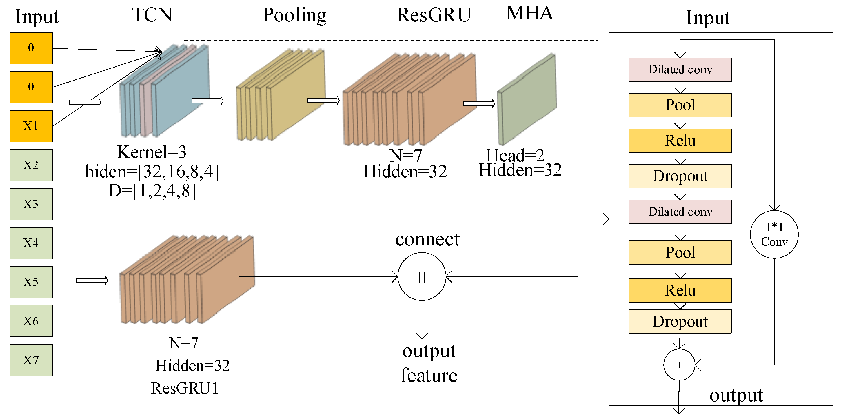
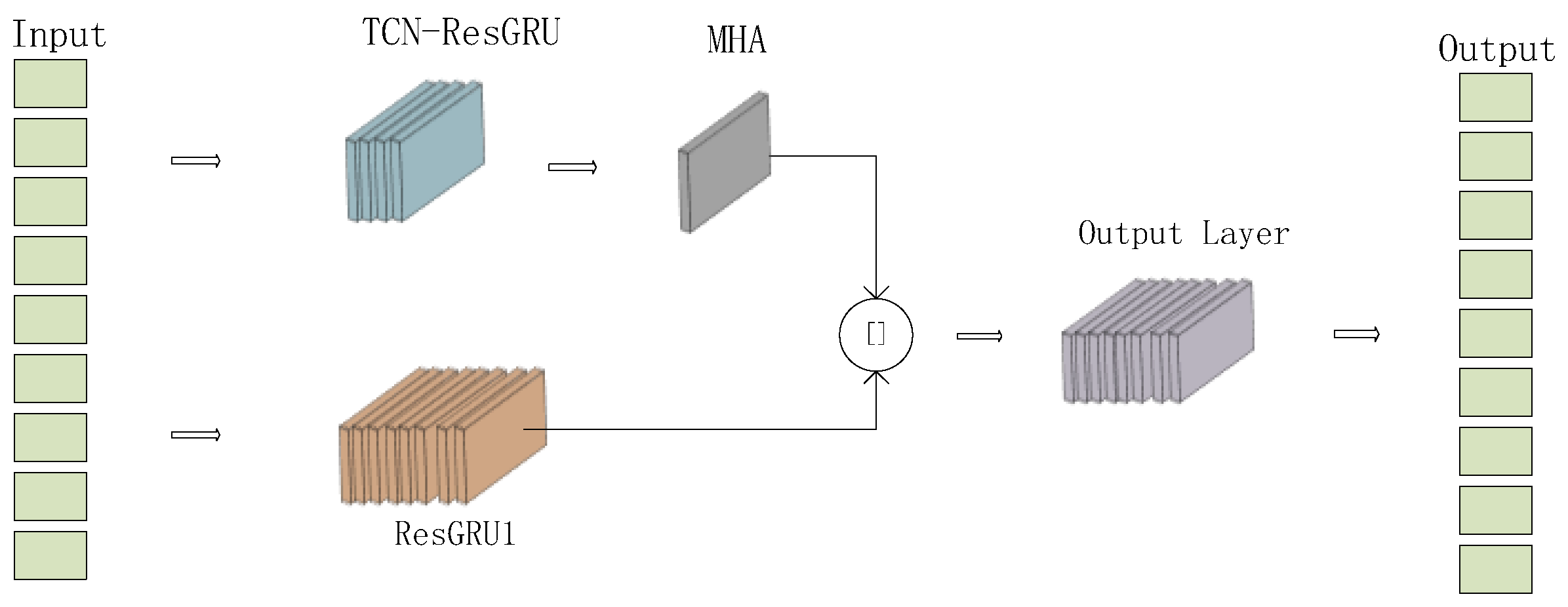
The model is divided into four modules: TCN-ResGRU network, ResGRU1 network, MHA mechanism, and output module. The first three modules are used to extract the track timing features, and the last module is used to calculate the output filter value. Figure 1 is as shown below.

Figure 1. Model diagram.

This chapter introduces each of the architectures shown in the diagram.

2.3.1. Temporal Convolutional Network

The temporal convolutional network (TCN) [46] is a convolutional neural network architecture dedicated to processing temporal data. By combining causal convolution, dilated convolution and residual connection, the TCN maintains the advantages of efficient parallel computing of convolutional neural networks. It overcomes the defect of a traditional CNN that struggles to capture long-term dependence. Compared with the traditional recurrent neural network (RNN) and its classical variants, the TCN has the following advantages in processing long sequence data: firstly, the parallel computing features greatly improve the training efficiency of the TCN; and secondly, the TCN can effectively capture the features of different time scales through the well-designed dilated convolution structure. Finally, the introduction of residual connection solves the problem of gradient vanishing in deep network training. These features enable the TCN to show excellent performance in speech recognition, action prediction, temporal prediction, and other fields. The core structure of the TCN is as follows:

• Causal convolution: Causal convolution is a fundamental component of the TCN, and its core idea is to ensure that the output of the moment depends only on the time $t$ and the input before the time $t$ strictly follows the causality of the temporal sequence. The convolution operation formula is as follows:

  $$A=\left(\begin{array}{ccc}{a}_{11}& a_{12}& a_{13}\\ a_{21}& a_{22}& a_{23}\\ a_{31}& a_{32}& a_{33}\end{array}\right)$$

  (22)

  $$X=\left(\begin{array}{ccc}{x}_{ij}& x_{ij+1}& x_{ij+2}\\ x_{i+1j}& x_{i+1j+1}& x_{i+1j+2}\\ x_{i+2j}& x_{i+2j+1}& x_{i+2j+2}\end{array}\right)$$

  (23)

  $$y_{ij}=\sum _{m=1}^3\sum _{n=1}^3{a}_{mn}{x}_{i+m-1 j+n-1}$$

  (24)
  With a convolution kernel size of $m\times n$ as an example, the matrix of $n=3$ is the length of the convolution kernel, $m=3$ is the width of the convolution kernel, the size of $m$ is consistent and invariant with the feature dimension, and the convolved matrix $h$ is wide to ensure that the input of each convolution operation contains all features. $n$ may vary, and is typically an odd number greater than 3. The difference between the causal convolution and the ordinary convolution is that the causal convolution is filled with 0 in the initial direction before the convolution operation, and the filling length is $n-1$, ensuring that only past and current track points are used to prevent future information leakage when calculating the convolution operation at each time step. The following demonstrates the difference between causal convolution and regular convolution:
  Suppose the time series to be convolved is $A$, with a sequence length of 5, given by $A=\{a_1,a_2,a_3,a_4,a_5\}$. The convolution kernel size is $3\times 3$, and we only consider the convolution along the time series direction. For causal convolution, $A$ is padded with a length of $3-1=2$, resulting in $A^{\prime }=\{{0, 0, a}_1,a_2,a_3,a_4,a_5\}$. When computing the first time step with causal convolution, the time series involved in the convolution is $\left\{{0, 0, a}_1\right\}$, where $a_1$ represents the track point at the first time step, and the $0$ represent the absence of track points before the first time step. At this time, $a_2$ represents future information. For regular convolution, the padding length is $3//2=1$, giving $\widehat{A}=\{{0, a}_1,a_2,a_3,a_4,a_5,0\}$, with padding applied at both ends. When computing the first time step, the time series involved in the convolution is $\{{0, a}_1,a_2\}$, and the presence of $a_2$ at this step indicates leakage of future information.
• Dilation convolution: In ordinary convolution operations, the size of the convolution kernel does not change, and the range of information accepted by each convolution is limited. In the dilated convolution, the convolution kernel is expanded by the blank region, so that a larger range of information can be extracted without increasing the parameters and the amount of calculation, and the missing information in the middle blank region can also be supplemented in the subsequent convolution, so that not only is part of the information not missed, but also the redundant information in the ordinary convolution operation can be effectively filtered. The dilated convolution is calculated as follows:

  $$y_{ij}=\sum _{m=1}^3\sum _{n=1}^3{a}_{mn}{x}_{i+m-1 j+d\times (n-1)}$$

  (25)
  Wherein the expansion coefficient $d$ represents the expansion size of the convolution kernel, and changes the size of the convolution kernel through the exponential growth of the expansion coefficient, so that the network can efficiently capture the multi-scale features from local to global.
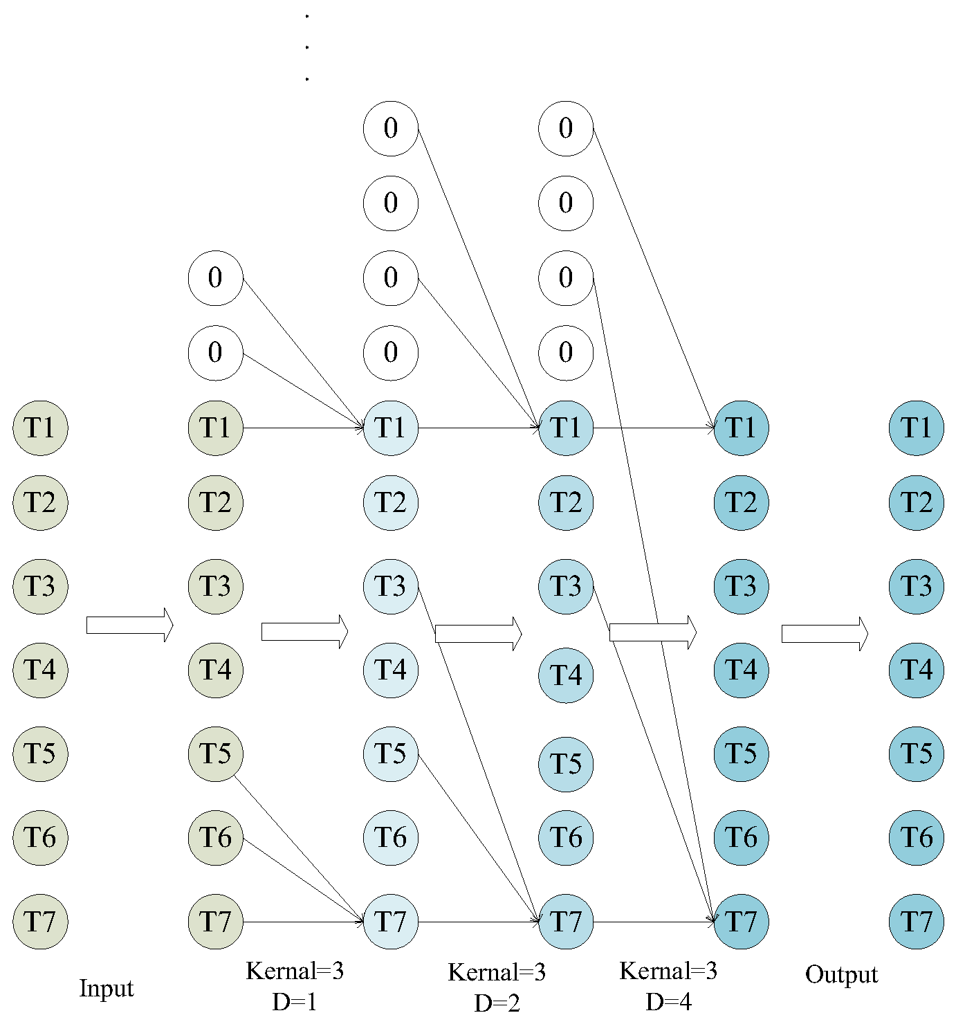
  As shown in the Figure 2, when the expansion coefficient $d=1$, the size of the convolution kernel is three columns, and there is no difference between the dilated convolution and the normal convolution. When the expansion coefficient $d=2$, the size of the convolution kernel is five columns; only the first, third, and fifth columns participate in the convolution operation, and the amount of calculation is unchanged, but the information (receptive field) in the range of five columns can be obtained by one convolution, and the missing information of the first convolution will be supplemented in the second convolution, which is less redundant than normal convolution operation. When the expansion coefficient $d=4$, the size of the convolution kernel is nine columns; only the first, fifth, and ninth columns are involved in the convolution operation, and the receptive field is further expanded.
  

  Figure 2. Schematic diagram of dilated convolution.

2.3.2. Residual Gated Recurrent Unit

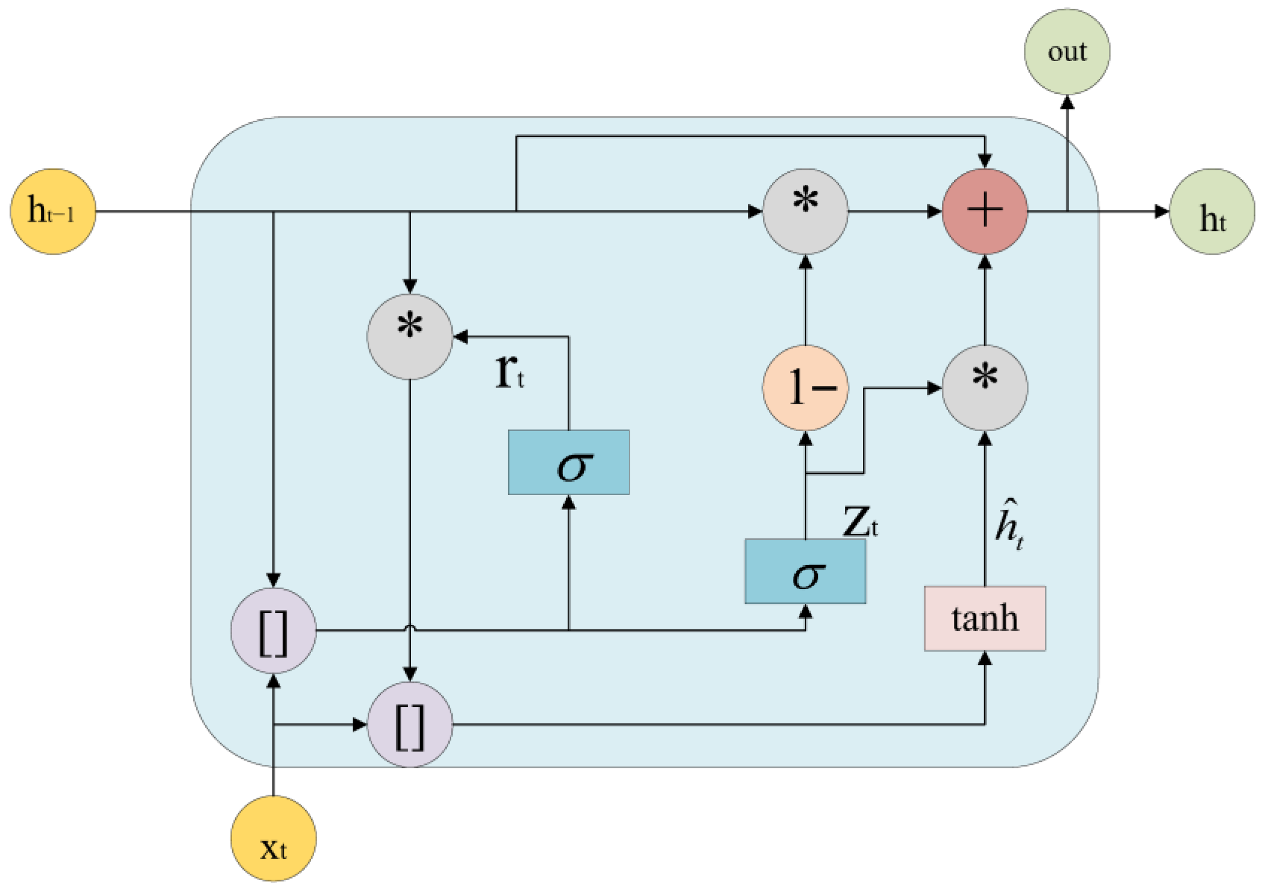
In this paper, we improve the GRU and introduce a residual module to propose a ResGRU network. The residual module transforms the original network from learning the features of each time step to learning the features of the difference between each time step. Let the original network input be $x$ and the output be $f\left(x\right)$; after introducing the residual network, the output is $H\left(x\right)=f\left(x\right)+x$. Available $f\left(x\right)=H\left(x\right)-x$, learning the original model from $x_t$ transformed into $x_t-x_{t-1}$. Time-dependent features can be better learned. At the same time $f\left(x\right)=0$, $H\left(x\right)=x$, this feature builds an identity network that further alleviates the gradient vanishing problem. Figure 3 is as follow:

Figure 3. Structure of residual gated recurrent unit. The colors are used to distinguish different functional modules. In the diagram, yellow represents input, green represents output, and the rest are all computational steps. Among “*” denotes the Hadamard product, multiplying the corresponding elements. “[]” indicates concatenation, concatenating data along a certain column so that the data’s dimensions remain un-changed, with the concatenated dimension being added. ‘1−’ means that the result obtained when the data passes through this region is ‘1 − x’.

Let the total time step length be $n$, the previous moment is characterized by $h_{t-1}$, the input at the current time is $x_t$, the reset gate weight matrix is $W_z$, the bias is $b_z$, update the gate weight matrix as $W_r$, the bias is $b_r$, the candidate state weight matrix is $W_h$, the bias is $b_h$, and the calculation steps are as follows:

• Calculate Reset Gate:

  $$z_t=\sigma (W_z·[h_{t-1},x_t]+b_z)$$

  (26)
  The reset gate controls how much the history information affects the current candidate state, where $\sigma$ express $sigmod$, the activation function is given by the following:

  $$\sigma (x)={\displaystyle \frac{1}{1+e^{-x}}}$$

  (27)
• Calculate Update Gate:

  $$r_t=\sigma (W_r·[h_{t-1},x_t]+b_r)$$

  (28)
  Determine the fusion ratio of new and old state information.
• Calculate candidate status:

  $${\widehat{h}}_t=tanh(W_h·[{r_t\ast h}_{t-1},x_t]+b_h)$$

  (29)
  Among $\ast$ denotes the Hadamard product, multiplying the corresponding elements.
• Calculate the final state:

  $$h_t=(1-z_t)\ast h_{t-1}+z_t\ast {\widehat{h}}_t+h_{t-1}$$

  (30)

2.3.3. Multi-Head Attention Mechanism

By parallelizing multiple groups of attention heads, this mechanism enables the model to focus on different representation subspaces of the input sequence at the same time, which significantly improves the modeling ability of the model for complex dependencies. In the task of track processing, MHA can simultaneously capture spatiotemporal multi-dimensional features, and its performance is far superior to that of traditional architecture. Enter the matrix $x\in R^{n\times d_{model}}$; the sequence length is $n$, and the model dimension is $d_{model}$. The calculation steps are as follows:

• Linear projection: each attention head $h$ to learn separate weight matrices, typically $d_k=d_v=d_{model}/H, W_h^Q\in R^{d_{model}\times d_k}, W_h^K\in R^{d_{model}\times d_k}, W_h^V\in R^{d_{model}\times d_v}$. The formula of calculation of $Q,K,V$ is as follows:

  $$Q_h=X{W}_h^Q$$

  (31)

  $$K_h=X{W}_h^K$$

  (32)

  $$V_h=X{W}_h^V$$

  (33)
• Parallel computing: compute each head $h$, compute the attention weight and the output, where the scaling factor $\sqrt{d_k}$ Prevent the dot product from being too large to cause the gradient to disappear, $softmax$ normalization is performed to generate a weight matrix. The formula is as follows:

  $$Attention(Q_h,K_h,V_h)=softmax({\displaystyle \frac{Q_h{K}_h^T}{\sqrt{d_k}}})V$$

  (34)
• Result fusion: the outputs of all heads are spliced and linearly transformed, and the formula is as follows:

  $$MultiHead(Q,K,V)=Concat({head}_1,{head}_2,\dots ,{head}_n)$$

  (35)
• Among ${head}_n=Attention(Q_h,K_h,V_h)$, $W^o\in R^{H{d}_o\times d_{model}}$ is the output weight matrix. After all the formulas are integrated, the following is obtained:

  $$MultiHead(X)=Concat(softmax({\displaystyle \frac{X{W}_h^Q{\left(X{W}_h^K\right)}^T}{\sqrt{d_k}}})X{W}_h^V{)}_{h=1}^H{W}^o$$

  (36)

2.4. Proposed Fusion Network Architecture

2.4.1. Temporal Feature Extraction Module

Temporal sequence is a series of data recorded in chronological order. The features of temporal sequence are hidden in different time segments, and the temporal features of data need to be fully considered in data analysis, which increases the difficulty of temporal sequence analysis. Temporal sequence usually has the features of high data dimension, large data noise, insufficient data, unknown time dependence span, and so on. Temporal research tasks include classification, clustering, and regression; the content of this paper belongs to the regression problem of temporal sequence [47]. The temporal sequence has the following features:

• Shape feature: This is the most intuitive feature in the time domain. The waveform of the sequence reflects the trend of the variable, and the waveform itself is the identifying feature of the sequence.
• Time-dependent feature: a hidden relationship between time steps, such as the information of the moment and the relationship between the information of the moment.
• Sequential transformation feature: a new representation that preserves the features of a temporal sequence or reduces the dimensionality of a temporal sequence. It is calculated by spatial transformation of the temporal sequence, suppressing the noise of the temporal sequence and completing the incomplete data [48].

The fusion network model proposed in this paper can effectively extract local and global temporal features through the multi-scale convolution kernel, dimension change in the multi-layer network, and weight re-division of multi-head attention. Figure 4 is as follow:

Figure 4. Flow chart of temporal feature extraction. The “*” here should be replaced with “×”, representing a convolution kernel size of 1 × 1. Here, “+” represents the addition of the two. “[]” indicates concatenation, concatenating data along a certain column so that the data’s dimensions remain unchanged, with the concatenated dimension being added.

Feature extraction: Temporal features are extracted from two dimensions: The architecture leverages the parallel processing capability of the TCN to achieve multi-scale long-range dependency modeling. Integrated with the residual learning mechanism and dynamic noise robustness of ResGRU, this hybrid framework effectively extracts spatiotemporal variation features ${feature}_{var}$ from input trajectory sequences. Enhanced by an MHA mechanism, the system attains adaptive high-dimensional feature weighting and spatiotemporal feature decoupling, thereby enabling explicit redistribution of sequence-level feature importance. At the same time, the ResGRU1 network is used to extract the shape and time-dependent features ${feature}_{shape+time}$ of the track data. The features are spliced to obtain the time sequence feature.

$$feature=connect[{feature}_{var},{feature}_{shape+time}]$$

(37)

This framework provides three core capabilities for processing asymmetric radar trajectories, distribution-invariant learning of coordinate transformation noise, rapid-response mechanisms for sudden maneuvers and transient noise events, and interpretable feature separation of high-dimensional non-Gaussian features, establishing itself as an effective computational framework for complex asymmetric sensor-derived data.

2.4.2. Location of Multi-Head Attention Mechanism

The position of the attention mechanism also has a significant influence on the filtering effect of the model. The attention mechanism is placed in different positions in the model. Figure 5 is as follow:

Figure 5. Location of MHA.

According to the figure, the MHA mechanism can select the above positions. To ensure the filtering effect, comparative experiments are conducted on different positions of the MHA mechanism.

Table 2 is as shown above. This experiment studies whether the position of the MHA mechanism in the model has an impact on the filtering results. It can be seen from the table that in the model without the MHA mechanism, the RMSE is 23.031 lower compared with the CNN-GRU. When the MHA mechanism is connected to ResGRU1, the RMSE is 173.2309 higher compared with the CNN-GRU. When the features are merged and then connected to the MHA mechanism, the RMSE is 77.3811 higher compared with the CNN-GRU. When the MHA is connected to the output module, the RMSE is 686.0465 higher compared with the CNN-GRU.

Table 2. Influence of attention mechanism position on filtering result.

Location	Distance (m)	MSE (m)	MAE (m)	RMSE (m)
No attention	173.0015	22,092.6914	111.1073	148.6361
Location A	165.3062	20,795.0762	106.1871	144.2050
Location B	408.5413	118,954.6484	259.8069	344.8980
Location C	294.1659	62,025.0117	187.4611	249.0482
Location D	1020.1211	735,672.6250	625.7421	857.7136
CNN-GRU	203.2122	29,469.5996	129.7452	171.6671

Experimental results show that the MHA mechanism in the proposed model structure has the best effect after being placed in the TCN-ResGRU, and the MHA mechanism reduces the RMSE by 4.4311. The MHA mechanism can be retained when the application scenario has high requirements on the filtering effect and low requirements on the model operation efficiency. When the application scenario has low requirements for filtering effect and high requirements for model operation efficiency, the MHA mechanism can be abandoned.

2.4.3. Filtering Value Computation

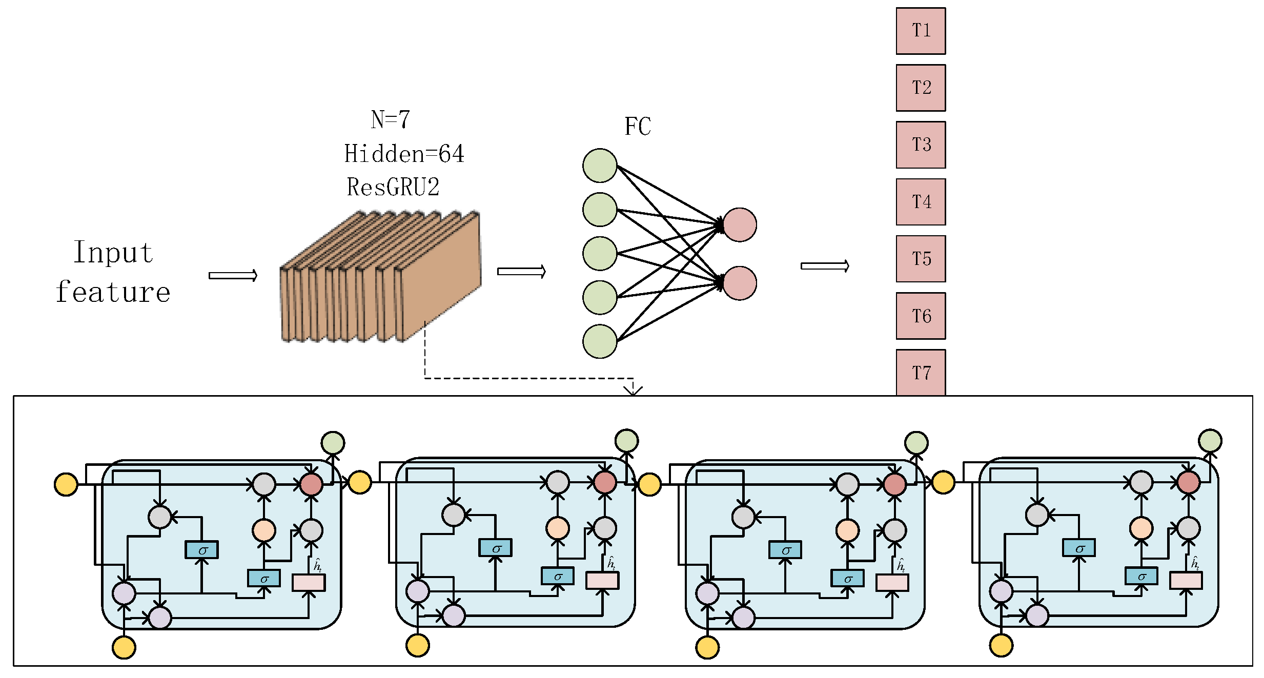
Filter Value Calculation: The calculation of the filter value mainly depends on the fully connected layer. The fully connected layer, also known as the Dense Layer, is one of the most basic and important components in deep learning. As the core building block of the neural network, the fully connected layer can realize the synthesis and conversion of global features, and realize the feature mapping of high-dimensional space by connecting each element of the input vector and the output vector. In the task of track processing, the fully connected layer is usually used as the final decision-making layer or feature fusion layer of the network, which undertakes the key conversion function from abstract features to concrete outputs. Figure 6 is as follow:

Figure 6. Chart of model calculation.

Use the ResGRU2 network to further extract temporal features from the feature values concatenated in the previous step. Use the fully connected layer output the result and map it to the real domain. Given input vector $X=feature$, weight matrix $W$, offset $B$, the calculation formula of the fully connected layer is as follows:

$$Y=X{W}^T+B$$

(38)

The filtering value calculation steps are as follows:

• Time data splitting: The input data is processed by using a gating recurrent unit to obtain the features of each time step ${feature}_t$;
• Dimensional Transformation and Filtered Value Mapping: Features at each time step using two fully connected layers ${feature}_t$ are processed to re-convert the feature dimensions of the results into two-dimensional coordinates $(x,y)$, and then the filtered values are mapped to the real domain.
• De-normalization: Since both the training set and the test set are normalized in the preprocessing, the output result needs to be de-normalized to obtain the final filtering value. The de-normalization calculation formula is as follows:

  $$x=x_{new}·\sigma +\mu$$

  (39)

2.5. Training Strategy

The experiment employs a rigorous training procedure to ensure the model’s reproducibility and generalization capability, with the specific strategies as follows:

The dataset is randomly split in a 7:2:1 ratio: Training Set 70%: Used for updating model parameters and feature learning. Validation Set 10%: Used to monitor the training process, trigger early stopping, and tune hyperparameters. Test Set 20%: Used only for final performance evaluation, without interacting with training. The splitting process ensures reproducibility with a fixed random $seed=42$ and preserves consistent class distribution through stratified sampling.

The network weights are initialized using He Initialization, which generates initial weights based on a Gaussian distribution $N~(0,{\displaystyle \frac{2}{nin}})$, where $nin$ is the number of input neurons. This effectively mitigates the gradient vanishing problem in ReLU-family activation functions and accelerates convergence.

Optimizer: Using the Adam algorithm (${\beta }_1=0.9$, ${\beta }_1=0.999$, $\epsilon ={10}^{-8}$) with an initial learning rate of $\eta =0.01$. Learning rate adjustment: Using the StepLR strategy, the learning rate is multiplied by a decay factor $\gamma =0.5$ every 100 training epochs, as per the following formula:

$$n_t=n_0\times {\gamma }^{{\displaystyle \frac{t}{s}}},s=100$$

(40)

The dynamic decay mechanism allows the model to fine-tune parameters in the later stages, enhancing convergence stability.

Batch Size: Set to 512 to balance memory efficiency and gradient estimation stability. Max Epochs: Limit to 1000 epochs to prevent indefinite training. Early Stopping: Monitor the validation loss, and if it does not decrease by more than $\delta ={10}^{-4}$ for 50 consecutive epochs, stop training and revert to the best weights. Loss Function: Use Mean Squared Error (MSE) for regression tasks.

$$MSE={\displaystyle \frac{1}{n}}\sum _{i=1}^1{(y_i-{\widehat{y}}_i)}^2$$

(41)

Here, $n$ is the number of samples in the batch, $y_i$ is the true value, and ${\widehat{y}}_i$ is the predicted value.

2.6. Data Preprocessing

During data preprocessing, it is necessary to adjust the size of the dataset. This article uses a sliding window to divide longer trajectories into fixed length trajectories, and at the same time divides the trajectory points of this length into feature values and labels. The steps are as follows:

• Let the original data be $S=\{s_1,s_2,\dots ,s_n\}$. The original data is three-dimensional data (target, feature, time series) stored in a two-dimensional table and converted into (target * feature, time series). The feature is (observation value $x^{\prime }$, observation value $y^{\prime }$, time $t$, true value $x$, true value $y$). Therefore, each five rows represents the trajectory of a target, and each column represents the feature of one time step of the trajectory. Set the feature value length, label value length, and sliding window length to $W$. The starting point of the sliding window is $i$, and the original data length is $n$, $s_i=[x_i^{\prime },y_i^{\prime },t_i,x_i,y_i]$.
• When $w+i\le n$ is present, extract five rows and columns of data with the starting column i and ending column w + i. The window size is $w$, after each data capture, the moving distance step is $k$, and the calculation formula is as follows:

  $$S_i=\left\{s_j\right|i\in [1,n-w],j\in [i,i+n]\}$$

  (42)
  When $w+i>n$, proceed to the next step.
• When $w+i>n$, stop translating the window. The final dataset $\widehat{S}$ is obtained by sequentially concatenating the data captured by each sliding window, and the calculation formula is as follows:

  $$\widehat{S}=[S_1,S_2,\dots ,S_n]$$

  (43)

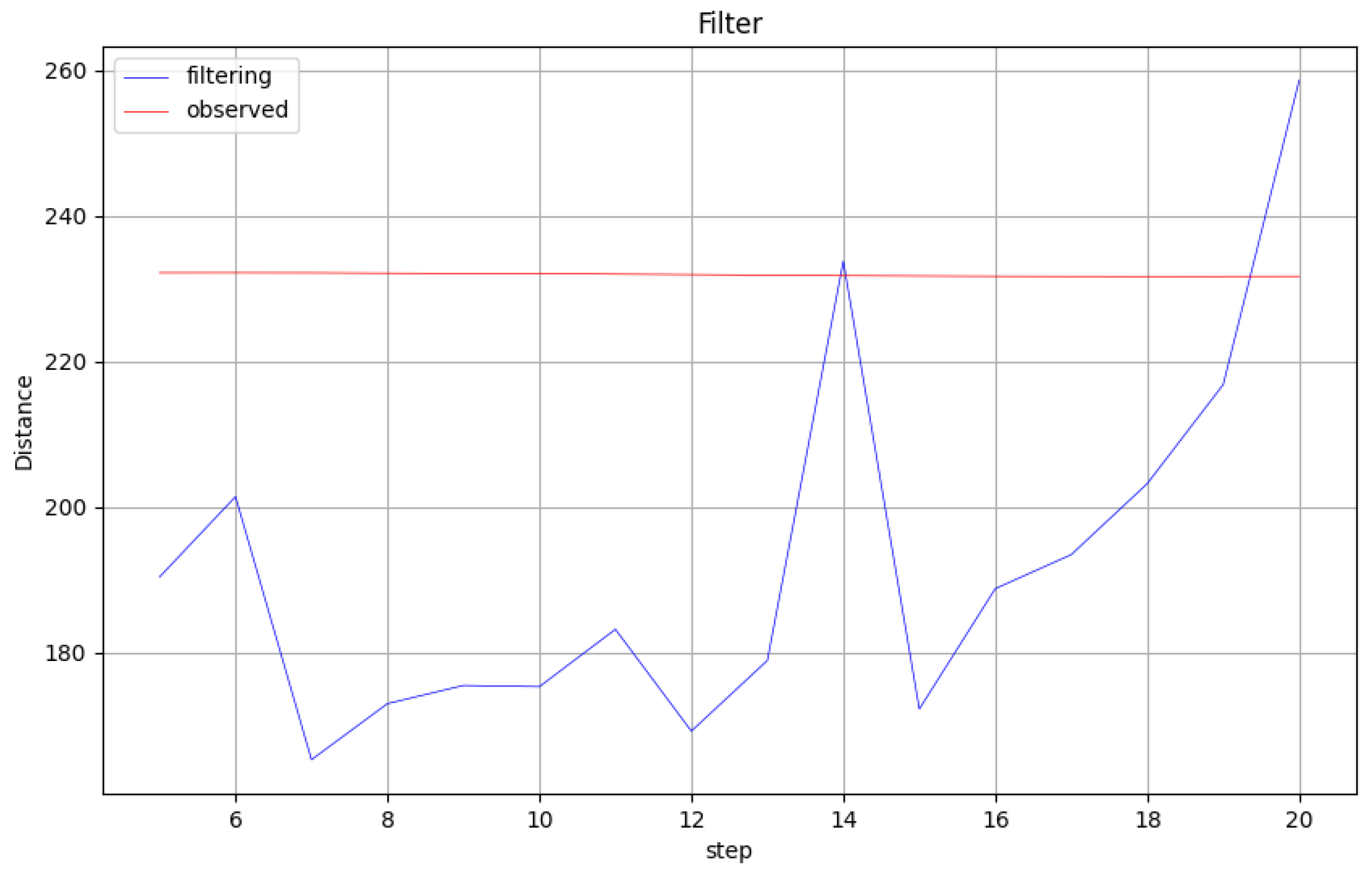
In different filtering step sizes $l$, the model is trained to obtain the influence of the filtering step on the filtering effect of the model. Figure 7 is as follow:

Figure 7. Schematic diagram of influence of filtering step on filtering.

This experiment focuses on the filtering step size of the model input data. $L$ the influence of the length on the filtering results is studied. Filtering step size $L$ indicates the number of track points of the observed track of the input model, and the output step length $N$ indicates the number of track points of the filtered track output by the model. Since the filtering step in this paper $L$ and output step $N$ are equal, only the filtering step size $L$ is used to express this.

The horizontal axis in the figure represents the filtering step $L$, the vertical axis represents the filtered range error, the red line represents the range error between the observed track and the true track, and the blue line represents the range error between the filtered track and the true track. It can be clearly observed that in $L=7$, the filtering effect is the best, whereas in $L=20$, the filtering effect is the worst, and the error exceeds the error between the observed track and the real track.

Experimental conclusion: Under normal circumstances, if the filtering step is too short, the model will not be able to learn the features of the track movement, and if the filtering step is too long, the useless information in the past will interfere with the calculation of the current filtering value. If there are no other special requirements for the application scenario, the filtering step should be set to $L=7$. When $L\ge 20$, the filtering effect is negative.

Radar scanning cycle refers to the time when the radar scans periodically and obtains the target coordinates. Since different radar models have different scanning cycles, the study investigates whether the simulated radar scanning cycle has an impact on the filtering results when generating simulation data. Table 3 is as follow:

Table 3. Influence of radar scanning period on filtering result.

Radar Cycle	Distance (m)	MSE (m)	MAE (m)	RMSE (m)
2	165.3062	20,795.0762	106.1871	144.2050
3	190.3916	26,453.3164	122.2505	162.6448
5	258.6139	48,986.9375	164.6061	221.3299
10	307.3570	87,285.5078	194.6360	295.4412
20	289.4915	63,946.5078	186.9411	252.8765

$T$ represents the radar scanning period. It can be seen from the table that when the simulation data is generated, the radar scanning cycle is simulated. When $T=2 s$, the filtering effect of the model is the best, and the average distance error of each track point is 165.3062 m. During the radar scan cycle $T=10$, the average distance error of each track point is 307.3570 m. The scanning period of radar affects the frequency of data acquisition. The shorter the scanning period of radar is, the more sufficient the data acquired in unit time is, and the more sufficient the feature extraction is. The longer the radar scanning cycle is, the less data collected in unit time, thus some features are missing. When the radar scanning cycle is too long, there are too many missing features, which means that the seven track points of the current input model contain multiple motion processes, thus interfering with the filtering calculation, and the filtering calculation is more random.

The experimental results show that the shorter the radar scanning period, the better the filtering effect. Radar scanning period $T>10$ s will cause the filtering calculation to be more random, which does not conform to the law that the filtering effect decreases with the increase in radar scanning period.

Standardization and de-standardization: There are two problems: whether the characteristic value is standardized and whether the label is standardized. The eigenvalue is not standardized, which leads to the slow convergence of model training, and the model is affected by the magnitude difference in eigenvalue data, resulting in low accuracy of track filtering. The label is not standardized: the filter value calculated by the model is the total result without standardization, but the convergence of model training is slow, and the accuracy of track filtering is low. Label standardization: The model has fast convergence during training and high accuracy of track filtering, but the filtering results need to be de-standardized. This paper finally adopts the strategy of standardization of eigenvalues and labels.

Track data is composed of different features, which are observed track coordinates, real track coordinates, and time steps. An observation track coordinate and a time step are obtained by splicing $(x_i^{\prime },y_i^{\prime },t_i),$ as $feature$; true track coordinates $(x_i,y_i)$ are obtained by splicing as $label$. Between the order of magnitude of $x_i^{\prime }$ and $y_i^{\prime }$ there is a big difference, which affects the accuracy of the model. Secondly, the data magnitude leads to the low speed of model training and prediction. In the stage of data preprocessing, there are two kinds of standardization methods to deal with data: maximum and minimum standardization method, and mean and variance standardization method. The max-min normalization method is sensitive to outliers. When the coordinates of an outlier exceed the maximum value or are less than minimum value, the coordinates of the outlier processed by the max-min normalization method are not in [0, 1], and the accuracy of track filtering is seriously reduced. There are two methods for data normalization in the model calculation stage: Layer Normalization (LN) and Batch Normalization (BN). After using an LN layer and a BN layer, the model has an obvious overfitting phenomenon, and the accuracy of the model effect in training and evaluation is quite different, so it is not used. In this paper, the mean variance standardization method is used to process the data in the data preprocessing stage, and the mean variance standardization formula is as follows:

$$x_{new}={\displaystyle \frac{x-\mu }{\sigma }}$$

(44)

$x_{new}$ is the result after standardization, $x$ is the input, $\mu$ is the mean of $x$, and $\sigma$ is the standard deviation of $x$. The model predicts the results and then de-standardizes them to obtain the real results. The de-normalization formula is as follows:

$$x=x_{new}·\sigma +\mu$$

(45)

We propose a fusion network architecture, but it is not clear why it is suitable and beneficial.

3. Experimental

3.1. Experimental Setup

3.1.1. Environment

Here, the experimental environment is introduced. Table 4 is as follow:

Table 4. Network parameters of TCN-ResGRU-MHA.

Layers	Parameter	Option
TCN layer	Kernel size	3
	Num of filters	32
	Activation	Relu
	padding	2
	Dilations	[32, 16, 8, 4]
ResGRU layer	hidden	32
	dropout	0.1
MHA layer	hidden	32
	Num of heads	2
ResGRU1 layer	hidden	32
	dropout	0.1
ResGRU2 layer	hidden	64
	dropout	0.1
Full connected layer	Num of filters	2
	Activation	Linear

The table provides detailed information on each network layer and its parameters in the TCN-ResGRU-MHA network architecture. Since the ResGRU network is used multiple times, the subsequent ResGRU network suffixes are increased by 1 or 2 for differentiation.

Here, the hyperparameter settings of TCN-ResGRU-MHA are introduced. Table 5 is as follow:

Table 5. Hyperparameters of TCN-ResGRU-MHA.

Parameter	Option
Batch size	512
dropout	0.1
Learning rate	0.01
Iterations	1000
Num of MHA heads	2
Loss function	MSE
optimizer	Adam

The table provides detailed information on the batch size, dropout, learning rate, number of iterations, number of attention heads in the MHA mechanism, loss function, and optimizer that are used during model training.

3.1.2. Dataset

The simulation data generation process is to simulate the data collection process in the real scenario. The real track is generated to represent the target’s own track and simulate the data from AIS. The observed track simulation uses the radar to detect the track of the target. To generate asymmetric radar track data, kinematic equations are parametrized to induce nonlinear trajectories, while sensor-specific observation noise is introduced within the polar coordinate system, emulating inherent radar ranging and bearing errors. Following acquisition in polar coordinates (range and azimuth), both the target observations and their associated errors reside natively in this domain. Consequently, the true Cartesian trajectory must be transformed to polar coordinates for the injection of simulated angular and range errors, replicating the radar’s measurement process. For subsequent analysis in Cartesian space, the noisy polar observations must undergo conversion back to Cartesian coordinates. The data simulation steps are as follows:

• Randomly generate target initial point and randomly generate acceleration $a$, initial speed $v_0$, angular acceleration $a_0$, initial angular velocity $v_{\theta }$, initial direction $\theta$, and initial coordinates $(x,y)$. Acceleration and angular acceleration are constant, while velocity, angular velocity, position, and direction are affected by higher-order physical quantities.
• The speed, the angular speed, the position, and the direction of the next time point are sequentially calculated according to the physical quantity. To obtain the true track, the formula is as follows:

  $$\Delta d={\displaystyle \frac{1}{2}}a\Delta t^2+v_{t-1}\Delta t$$

  (46)

  $$v_t=v_{t-1}+a\Delta t$$

  (47)

  $$v_{\theta }=v_{{\theta }_{t-1}}+a_{\theta }\Delta t$$

  (48)

  $${\theta }_t={\theta }_{t-1}+{\displaystyle \frac{1}{2}}{a}_{\theta }{\Delta t}^2+v_{{\theta }_{t-1}}\Delta t$$

  (49)

  $$x^{\prime }=x+\Delta d\mathit{cos}{\theta }_{t-1}$$

  (50)

  $$y^{\prime }=y+\Delta d\mathit{sin}{\theta }_{t-1}$$

  (51)

  $$F_k={[x_k,y_k,v_k,{\theta }_k,v_{\theta k}]}^T$$

  (52)

  $${\widehat{F}}_{\mathrm{k}}=\left[\begin{array}{ccc}\begin{array}{ccc}1& 0& \Delta tcos{\theta }_k\end{array}& 0& 0\\ \begin{array}{ccc}0& 1& \Delta tcos{\theta }_k\end{array}& 0& 0\\ \begin{array}{c}\begin{array}{ccc}0& 0& 1\end{array}\\ \begin{array}{ccc}0& 0& 0\end{array}\\ \begin{array}{ccc}0& 0& 0\end{array}\end{array}& \begin{array}{c}0\\ 1\\ 0\end{array}& \begin{array}{c}0\\ \Delta t\\ 1\end{array}\end{array}\right]F_k+a_{\theta }[\begin{array}{c}0\\ \begin{array}{c}0\\ 0\\ \begin{array}{c}{\displaystyle \frac{1}{2}}\Delta t^2\\ \Delta t\end{array}\end{array}\end{array}]+a[\begin{array}{c}{\displaystyle \frac{1}{2}}\Delta t^{2}cos{\theta }_k\\ \begin{array}{c}{\displaystyle \frac{1}{2}}\Delta t^{2}cos{\theta }_k\\ \Delta t\\ \begin{array}{c}0\\ 0\end{array}\end{array}\end{array}]$$

  (53)

  $$Z_k={[w_{\theta k},w_{rk}]}^T$$

  (54)
  $v_{t-1}$ and $v_{{\theta }_{t-1}}$ are the speed and angular velocity at the previous moment, respectively, and $\Delta t$ represents the time difference between the two trajectory points.$F_k$ is the state vector, $Z_k$ is the noise vector, and ${\widehat{F}}_{\mathrm{k}}$ is the updated state vector.
• Transforming the real track from the rectangular coordinate system to the polar coordinate system:

  $$\vartheta =\left\{\left.\begin{array}{c}arctan({\displaystyle \frac{y^{\prime }}{x^{\prime }}}),(x^{\prime }\ge 0)\\ arctan({\displaystyle \frac{y^{\prime }}{x^{\prime }}})+\pi ,(x^{\prime }<0)\end{array}\right\}\right.$$

  (55)

  $$R=\sqrt{{x^{\prime }}^2+{y^{\prime }}^2}$$

  (56)
  $(x^{\prime },y^{\prime })$ is the updated coordinate, $\vartheta$ is the updated angle, and $R$ is the updated distance.
• The true track in the polar coordinate system adds the angle error of the normal distribution with $\mu =0$ and $\sigma =0.2$ (degree). Add a distance error with $\mu =0$ and $\sigma =100$ (m), as follows:

  $${\theta }^{\prime }=\theta +w_{\theta }$$

  (57)

  $$R^{\prime }=R+w_r$$

  (58)
  ${\theta }^{\prime }$ is the angle that increases the observation noise, $R^{\prime }$ is the distance that increases the observation noise, $w_{\theta }=N~(0, 0.2)$ is the angular observation noise, and $w_r=N~(0, 100)$ is the distance observation noise.
• The track with radar observation error is converted from the polar coordinate system to the rectangular coordinate system to obtain the observation track, and the calculation formula is as follows:

  $$\widehat{x}=R^{‘}cos{\theta }^{’}$$

  (59)

  $$\widehat{y}=R^{‘}sin{\theta }^{’}$$

  (60)
  $(\widehat{x},\widehat{y})$ is the observed coordinate.

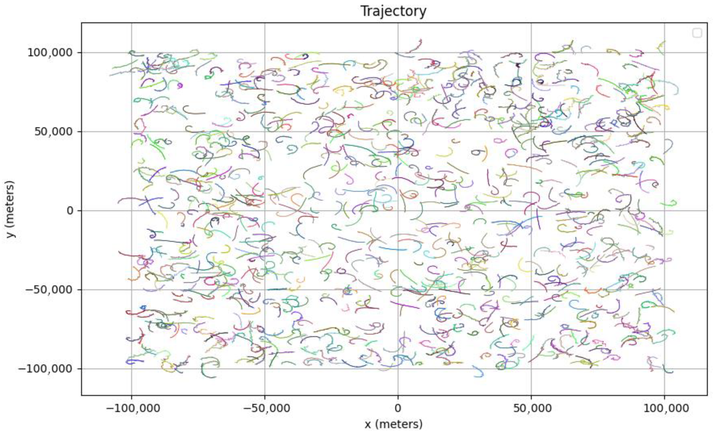
Due to space limitation, only 20 track points of 1000 targets selected in one group of the training set are displayed. Figure 8 is as follow:

Figure 8. Examples of training sets.

The differently colored line segments in the figure represent the trajectory of a target. The trajectory generation formula has been introduced earlier, and below we will explain the parameters of the formula.

Table 6 is as shown above. According to the above parameters, the starting position of the trajectory is randomly generated within a square area, the target acceleration and angular acceleration remain in the ranges of [−0.5 g, 3 g] ($\mathrm{m}/{\mathrm{s}}^2$) and [−0.5, 0.5] ($°/{\mathrm{s}}^2$), respectively, the initial magnitudes of velocity, angular velocity, and direction are in the ranges of [−2, 2] ($°/\mathrm{s}$), the radar scan period is simulated as 2(s), the number of target trajectory points is 100, the radar angle observation noise follows a normal distribution of $N~(0,0.2)$, the radar distance observation noise follows a normal distribution of $N~(0,0.2)$, the number of targets in the training set is ${7\times 10}^5$, and the number of targets in the test set is ${2\times 10}^5$.

Table 6. Table of simulation dataset production parameters.

Parameter	Training Set	Test Set
$X\text{-}\mathrm{axis} (\mathrm{m}$)	$[-{10}^6,{10}^6]$	$[-{10}^6,{10}^6]$
$Y\text{-}\mathrm{axis} (\mathrm{m}$)	$[-{10}^6,{10}^6]$	$[-{10}^6,{10}^6]$
$\mathrm{initial} \mathrm{velocity} (\mathrm{m}/\mathrm{s}$)	$[50, 500]$	$[50, 500]$
$\mathrm{Initial} \mathrm{direction} (°$)	$[0, 360]$	$[0, 360]$
$\mathrm{Acceleration} (\mathrm{m}/{\mathrm{s}}^2$)	[−0.5 g, 3 g]	[−0.5 g, 3 g]
$\mathrm{angular} \mathrm{velocity} (°/\mathrm{s}$)	[−2, 2]	[−2, 2]
$\mathrm{angular} \mathrm{acceleration} (°/{\mathrm{s}}^2$)	[−0.5, 0.5]	[−0.5, 0.5]
$\mathrm{Radar} \mathrm{scanning} \mathrm{cycle} (\mathrm{s}$)	2	2
trajectory points	100	100
$\mathrm{Distance} \mathrm{noise} (\mathrm{m}$)	$N~(0, 100)$	$N~(0, 100)$
$\mathrm{Angle} \mathrm{noise} (°$)	$N~(0, 0.2)$	$N~(0, 0.2)$
Num of Target	${7\times 10}^5$	${2\times 10}^5$

3.2. Evaluation Metrics

There are two steps in deep learning that need to be evaluated. The first is to use the loss value to evaluate the “distance” between the filter value and the label when training the model. The other is to evaluate the overall performance of the model when evaluating the model. Because of the different uses, the evaluation functions used in these two steps are also different.

Training: This paper uses the mean square error as the loss function to evaluate the accuracy of the model when training the model. The mean square error as the common loss function of the regression model has the advantages of fast convergence and effective reflection of the difference between the filter value and the label [23]. The calculation formula is as follows:

$$MSE={\displaystyle \frac{1}{n}}\sum _{i=1}^1{(y_i-{\widehat{y}}_i)}^2$$

(61)

Evaluation: This paper uses the average Euclidean distance, MSE, MAE, and RMSE to evaluate the accuracy of the model. Because the distance is more practical in practical application scenarios, the average Euclidean distance as an evaluation function is more practical. The calculation formula is as follows:

$$D={\displaystyle \frac{1}{n}}\sum _{i=1}^1{{(x_i-{\widehat{x}}_i)}^2+(y_i-{\widehat{y}}_i)}^2$$

(62)

$$MSE={\displaystyle \frac{1}{n}}\sum _{i=1}^1{(y_i-{\widehat{y}}_i)}^2$$

(63)

$$MAE={\displaystyle \frac{1}{n}}\sum _{i=1}^1{|y}_i-{\widehat{y}}_i|$$

(64)

$$RMSE=\sqrt{{\displaystyle \frac{1}{n}}\sum _{i=1}^1{(y_i-{\widehat{y}}_i)}^2}$$

(65)

After the model training is completed, use the evaluation mode to evaluate the model, and input the processed test set to obtain the filtered track.

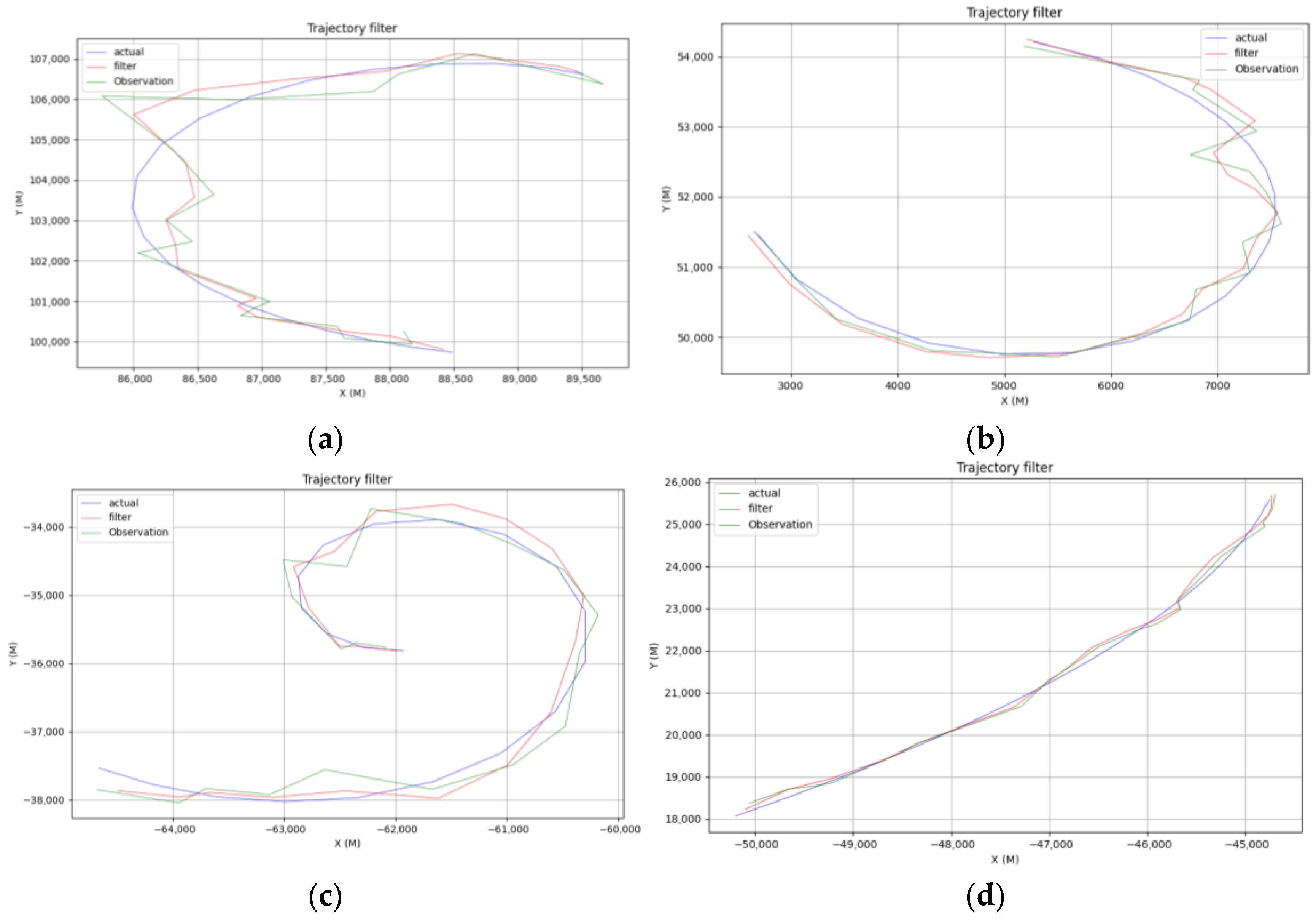
As shown in Figure 9, the figure shows the filtering results of a target using the TCN-ResGRU-MHA model proposed in this paper. The horizontal axis represents a rectangular coordinate system x-axis, vertical axis represents the y-axis, and there are zero simulated radar coordinates. Blue is the true track, green is the observed track, and red is the filtered track. Use the evaluation function to calculate the Euclidean distance between the filtered trajectory and the true trajectory, as well as between the observed trajectory and the true trajectory. By comparing the two, it can be seen that the model proposed in this paper is effective in filtering noise. The Figure 9 shows that the filtering effect has high accuracy in both linear and curved motion, e.g., (a–c) demonstrates the effectiveness of this model in curvilinear motion; (d) demonstrate the effectiveness of this model in approximate linear motion.

Figure 9. Schematic diagram of filtering results.

3.3. Comparative Analysis

Comparing the model in this paper with the traditional deep learning method.

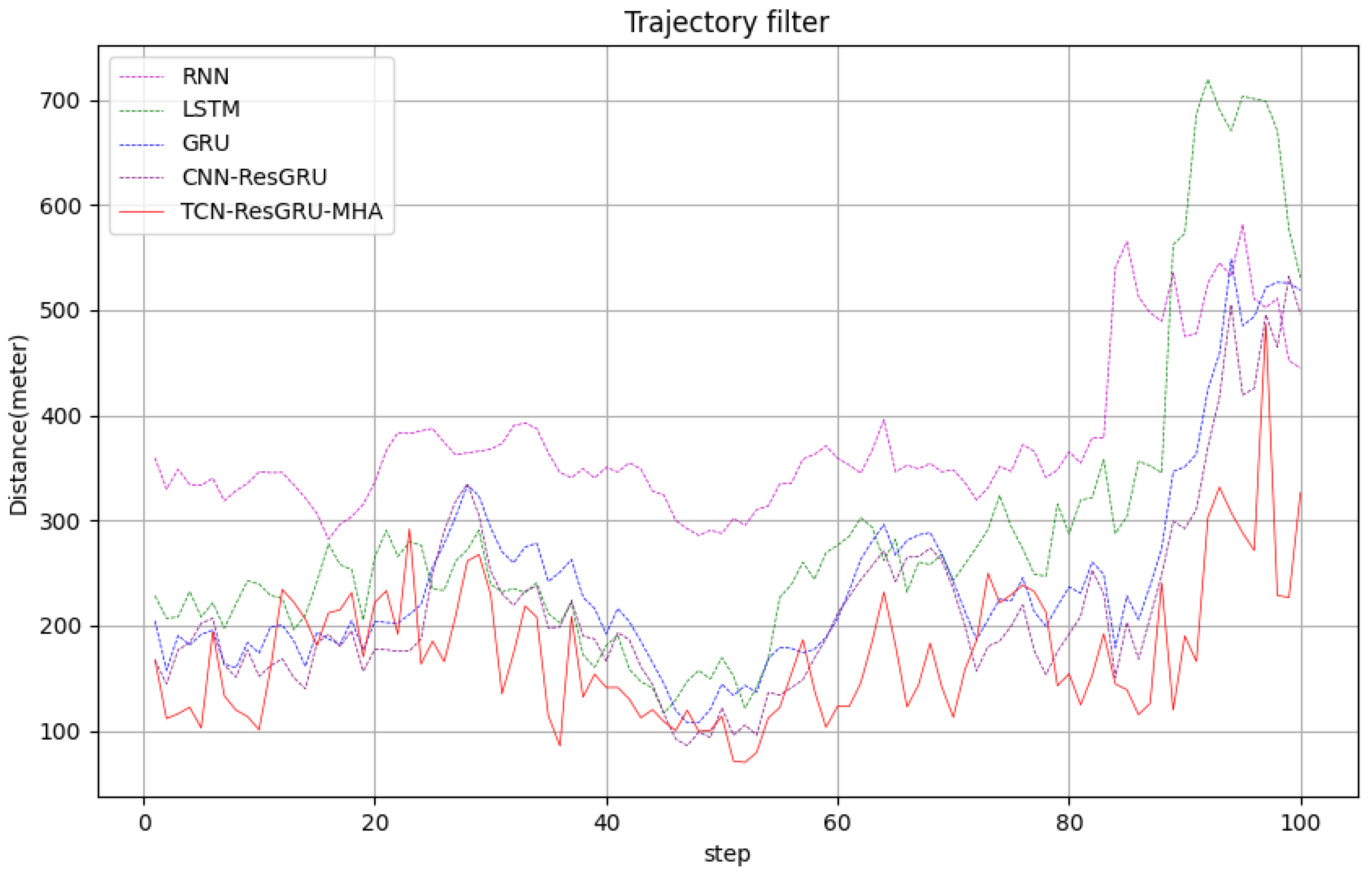
Table 7 is as shown above. In this experiment, the new track filtering algorithm based on the TCN-ResGRU-MHA proposed in this paper is compared with the traditional deep learning algorithm. It can be seen from the table that the structure proposed in this paper has a higher accuracy, where the RMSE is 108.6715 lower than the RNN, 37.0967 lower than LSTM, and 44.002 lower than GRU. Compared with CNN-GRU network, the RMSE is reduced by 27.4621. Although its computation time is 6.31 ms, it still meets real-time requirements. Figure 10 is as follow:

Table 7. Experimental comparison table.

Model	Distance (m)	MSE (m)	MAE (m)	RMSE (m)	Increase	Time (ms)
RNN	289.4915	63,946.5078	186.9411	252.8765	−47.30%	1.33
LSTM	206.6974	32,870.2969	133.7415	181.3017	−5.61%	1.27
GRU	217.3204	35,421.8594	140.1020	188.2070	−9.63%	1.29
CNN-GRU	203.2122	29,469.5996	129.7452	171.6671	0%	1.99
TCN-ResGRU-MHA	165.3062	20,795.0762	106.1871	144.2050	15.99%	6.31

Figure 10. Comparison chart of each model.

In the figure, the horizontal axis represents the serial number of the test set, and the vertical axis represents the filtering distance error calculated for the set of test sets using the model. The purple dotted line, green dotted line, blue dotted line, and red solid line in the figure, respectively, represent the filtering results of the RNN, LSTM network, GRU network, and TCN-ResGRU-MHA network. It can be clearly seen that the red solid line is at the bottom; the filtering distance error is the smallest, and the filtering effect is better than other traditional deep learning networks in the figure.

Experimental conclusion: Compared with the traditional deep learning algorithms such as the RNN, LSTM network, GRU network and CNN-GRU network, the new algorithm based on TCN-ResGRU-MHA has better filtering effect.

3.4. Ablation Study

To investigate whether each module in the network architecture proposed in this paper contributes to the results, ablation experiments were conducted.

Table 8 is shown above. It can be seen from the table that when the structures in the model are complete, the minimum average RMSE of the filtered track is 144.2050 m, which is 27.4621 lower than that of the CNN-GRU. When the TCN-ResGRU network, ResGRU1 network, MHA mechanism and ResGRU2 network are canceled, the RMSE of the filtered track compared with the CNN-GRU are reduced by −120.039, −1003.5139, 25.5011, and −11.4331, respectively.

Table 8. Ablation test table.

Model	Distance (m)	MSE (m)	MAE (m)	RMSE (m)
All structures	165.3062	20,795.0762	106.1871	144.2050
No TCN-ResGRU	343.5904	85,092.4766	217.0534	291.7061
No ResGRU1	1349.9578	1,381,050.3750	836.4162	1175.1810
No MHA	172.2606	21,364.4883	110.2944	146.1660
No ResGRU2	216.8290	33,525.6953	138.4370	183.1002
CNN-GRU	203.2122	29,469.5996	129.7452	171.6671

Experimental results show that each module of the model has a positive effect on the track filtering algorithm, and the importance of each module is in the following order: ResGRU1 network, TCN-ResGRU network, ResGRU2 network, and MHA mechanism. The MHA mechanism has the least improvement on the track filtering effect, and the MHA mechanism can be retained when the application scenario has high requirements on the filtering effect and low requirements on the model operation efficiency. When the application scenario has low requirements for the filtering effect and high requirements for the model operation efficiency, the MHA mechanism can be abandoned.

3.5. Parameter Sensitivity Analysis

Under the default parameters for MHA heads, TCN layer, learning rate, and batch size, the effect of changing each individual factor on the filtering performance is studied. Table 9 is as follow:

Table 9. Effect of parameters on filtering.

Parameters	MHA Heads	Distance (m)	MSE(m)	MAE (m)	RMSE (m)
MHA Heads	1	178.9278	23,266.0234	114.5371	152.5320
	2	165.3062	20,795.0762	106.1871	144.2050
	4	175.4966	22,175.2402	112.6373	148.9135
	8	183.2099	24,389.1582	117.2338	156.1703
TCN Layer	[8, 4]	188.7943	25,553.6816	120.8505	159.8552
	[16, 8, 4]	169.2244	21,220.4883	108.5608	145.6725
	[32, 16, 8, 4]	165.3062	20,795.0762	106.1871	144.2050
	[64, 32, 16, 8, 4]	175.3335	22,322.1641	112.2755	149.4060
Learning Rate	0.1	NA	NA	NA	NA
	0.05	NA	NA	NA	NA
	0.03	408.5413	118,954.6484	259.8069	344.8980
	0.01	165.3062	20,795.0762	106.1871	144.2050
	0.001	231.9032	37,707.9648	147.9353	194.1854
	0.0001	246.3875	41,715.6211	157.6332	204.2440
Batch Size	128	226.8642	35,736.6445	144.9219	189.0414
	256	193.4680	26,579.5488	123.6158	163.0323
	512	165.3062	20,795.0762	106.1871	144.2050
	1024	190.3916	26,453.3164	122.2505	162.6448

From the table above, it can be seen that the learning rate has the greatest effect on the filtering, followed by the batch size. It is recommended that parameter MHA heads take the values $[2, 4]$, the TCN layer takes the values $[32, 16, 8, 4]$ or $[16, 8, 4]$, learning rate takes the values $[0, 0.01]$, and batch size take the values $[256, 512]$.

4. Discussion

The proposed TCN-ResGRU-MHA architecture processes the raw data in parallel using the TCN, expands the receptive field through dilated convolutions, and obtains temporal features at different scales using different dilation factors. Causal convolutions are used to ensure that future information is not leaked. The residual module is introduced based on GRU, making it more effective at capturing short-term dynamic changes, ensuring a rapid response at points of abrupt signal changes, while suppressing gradient vanishing problems caused by deep network degradation. The multi-head attention mechanism is introduced to dynamically reassign feature weights, focusing on important moments, suppressing noise, reducing attention weights on outliers, and integrating multi-scale features. Multiple attention heads can focus on different time scales.

We analyze the computational complexity of the TCN-ResGRU-MHA hybrid network model, comparing the complexity of the TCN with that of a CNN structure achieving the same receptive field. Assuming the CNN has $n$ layers, L represents the length of the time series, and K represents the size of the convolution kernel, its receptive field is $2(n-1)+k$, while TCN requires $x$ layers to reach this receptive field. Working backward from the receptive field size, the receptive field from layer $x$ to layer $x-1$ is $2^{(x-1)}(k-1)+1$, and similarly, from layer $x-1$ to $x-2$ it is $2^{(x-2)}(k-1)+1$, and from layer $2$ to layer 1 it is $2^{(x-x)}(k-1)+1$. Thus, the total receptive field from layer $1$ to layer $x$ is ${\sum }_{i=1}^x{2}^{(x-i)}(k-1)+1=x-1+(k-1){\sum }_{i=1}^x{2}^{(x-i)}=x-1+(k-1)(2^x-1)$. Setting $x-1+(k-1)(2^x-1)=2(n-1)+k$, and ignoring constants and lower-order terms for computational complexity, we obtain $x\approx logn$. Typically, the computational complexity of a single CNN layer is $O(C_{in}·C_{out}·l·k)$, since $C_{in}$ and $C_{out}$ are constants, representing the number of input channels and output channels. The complexity of a single CNN layer is $O(l·k)$, and for $n$ layers it is $O(n·l·k)$. In contrast, the TCN achieving the same receptive field has a computational complexity of $O(l·k·logn)$. Since the ResGRU used has the same computational complexity as the GRU, no further analysis is performed on it. We then analyze the computational complexity of multi-head attention. Let $l$ be the length of the input time series, $d=C_{out}$ be the feature dimension and $h$ be the number of heads. According to the calculation formula mentioned earlier, the computational complexity for each head is $O(2n^2{\displaystyle \frac{d}{h}})$. The sum of computational complexity for all heads is $O\left(4n^{2}d\right)$.

The proposed model still has shortcomings. While the introduction of the MHA mechanism increases filtering accuracy, it also leads to higher computational complexity. The dilated convolution layers in the TCN require extensive training data and have a significant overfitting risk; performance collapses in small-data scenarios. On datasets with fewer than 10,000 samples, the overfitting degree is five times higher than CNN-GRU. Periodic noise suppression is insufficient, and the MHA mechanism lacks the ability to identify periodic stationary noise.

This architecture is more suitable for scenarios such as intensive care in cloud-based big data centers and high-precision industrial inspections. In resource-constrained or special signal characteristic scenarios, targeted degradation modifications are needed. In edge scenarios, MHA can be removed and replaced with lightweight Squeeze-Excitation attention. In small-data scenarios, part of the TCN layers can be frozen, and pre-trained convolutional features can be used. For real-time systems, the TCN can be replaced with causal dilated convolutions.

5. Conclusions

The proposed TCN-ResGRU-MHA trajectory filtering algorithm provides three core capabilities for processing asymmetric radar trajectories:

• Distribution-invariant learning of coordinate transformation noise,
• Rapid-response mechanisms for sudden maneuvers and transient noise events,
• Interpretable feature separation of high-dimensional non-Gaussian features,

Establishing itself as an effective framework for complex asymmetric sensor-derived data, it effectively solves issues that traditional deep learning filtering algorithms struggle with, including capturing long-term dependencies in high-dimensional spaces, often exhibiting high computational complexity, slow response to transient signals, and compromised noise suppression due to their inherent architectural asymmetries.

Our future work will focus on the following planned improvements:

• Lightweight Architecture: We will investigate replacing the TCN with more efficient models (e.g., Structured State Space, Octave Convolution) and compressing the MHA module using Linformer to reduce computational overhead.
• Multi-Sensor Fusion: The model’s capability will be expanded from single-sensor sequences to a framework that fuses information from diverse sources like radar, electro-optical, and ADS-B.
• Enhanced Interpretability: We will address the “black box” limitation by developing methods to improve model transparency, which is crucial for deployment in safety-critical applications such as air traffic control.

References

1. Zhu, H.; Tong, Q.; Hu, J.; Liu, X.; Hou, S. Altitude aware trajectory prediction methods for non towered terminal airspace. Sci. Rep. 2025, 15, 26810. [Google Scholar] [CrossRef]
2. Xinping, X.; Fangxue, Z.; Mingyun, G. Multi-dimensional neural network grey model with delay for intelligent ship trajectory forecasting. Appl. Math. Model. 2026, 150, 116497. [Google Scholar] [CrossRef]
3. Billah, M.M.; Zhang, J.; Zhang, T. A Method for Vessel’s Trajectory Prediction Based on Encoder Decoder Architecture. J. Mar. Sci. Eng. 2022, 10, 1529. [Google Scholar] [CrossRef]
4. Xue, H.; Chai, T. Vessel Track Prediction Based on Fractional Gradient Recurrent Neural Network with Maneuvering Behavior Identification. Sci. Program. 2021, 2021, 5526082. [Google Scholar] [CrossRef]
5. Volkova, T.A.; Balykina, Y.E.; Bespalov, A. Predicting Ship Trajectory Based on Neural Networks Using AIS Data. J. Mar. Sci. Eng. 2021, 9, 254. [Google Scholar] [CrossRef]
6. Alizadeh, D.; Alesheikh, A.A.; Sharif, M. Vessel Trajectory Prediction Using Historical Automatic Identification System Data. J. Navig. 2020, 74, 156–174. [Google Scholar] [CrossRef]
7. Jianming, L. Prediction Method of Ship’s Track Based on Mathematical Model. J. Coast. Res. 2020, 112 (Suppl. S1), 379–382. [Google Scholar] [CrossRef]
8. Cao, Y.; Cao, J.; Zhou, Z. Track Segment Association Method Based on Bidirectional Track Prediction and Fuzzy Analysis. Aerospace 2022, 9, 274. [Google Scholar] [CrossRef]
9. Chen, Y.; Yang, S.; Suo, Y.; Zheng, M. Ship Track Prediction Based on DLGWO-SVR. Sci. Program. 2021, 2021. [Google Scholar] [CrossRef]
10. Li, H.; Si, Y.; Zhang, Q.; Yan, F. 4D Track Prediction Based on BP Neural Network Optimized by Improved Sparrow Algorithm. Electronics 2025, 14, 1097. [Google Scholar] [CrossRef]
11. Chen, X.; Meng, X.; Zhao, Y. Genetic algorithm to improve Back Propagation Neural Network ship track prediction. J. Phys. Conf. Ser. 2020, 1650, 032133. [Google Scholar] [CrossRef]
12. Song, L.; Shengli, W.; Dingbao, X. Radar track prediction method based on BP neural network. J. Eng. 2019, 2019, 8051–8055. [Google Scholar] [CrossRef]
13. Zhou, H.; Chen, Y.; Zhang, S. Ship Trajectory Prediction Based on BP Neural Network. J. Artif. Intell. 2019, 1, 29–36. [Google Scholar] [CrossRef]
14. Zheng, Y.; Lv, X.; Qian, L.; Liu, X. An Optimal BP Neural Network Track Prediction Method Based on a GA–ACO Hybrid Algorithm. J. Mar. Sci. Eng. 2022, 10, 1399. [Google Scholar] [CrossRef]
15. Yin, Y.; Zhang, S.; Zhang, Y.; Zhang, Y.; Xiang, S. Aircraft trajectory prediction in terminal airspace with intentions derived from local history. Neurocomputing 2025, 615, 128843. [Google Scholar] [CrossRef]
16. Zhao, Y.; Li, K. A Fractal Dimension Feature Model for Accurate 4D Flight-Trajectory Prediction. Sustainability 2023, 15, 1272. [Google Scholar] [CrossRef]
17. Huang, M.; Ochieng, W.Y.; Macias, J.J.E.; Ding, Y. Accuracy evaluation of a new generic Trajectory Prediction model for Unmanned Aerial Vehicles. Aerosp. Sci. Technol. 2021, 119, 107160. [Google Scholar] [CrossRef]
18. Zheng, X.; Peng, X.; Zhao, J.; Wang, X. Trajectory Prediction of Marine Moving Target Using Deep Neural Networks with Trajectory Data. Appl. Sci. 2022, 12, 11905. [Google Scholar] [CrossRef]
19. Zhang, J.; Li, Z.; Luo, X.; Zhao, Y.; Lu, F. Study of Urban Unmanned Aerial Vehicle Separation in Free Flight Based on Track Prediction. Appl. Sci. 2024, 14, 5712. [Google Scholar] [CrossRef]
20. Chen, W.; Sang, H.; Zhao, Z. CWGCN: Cascaded Wavelet Graph Convolution Network for pedestrian trajectory prediction. Comput. Electr. Eng. 2025, 127, 110609. [Google Scholar] [CrossRef]
21. Alanis, A.Y. Exploring Kalman Filtering Applications for Enhancing Artificial Neural Network Learning. Algorithms 2025, 18, 587. [Google Scholar] [CrossRef]
22. Rosales, C.D.; Tosetti, S.R.; Soria, C.M.; Rossomando, F.G. Neural Adaptive PID Control of a Quadrotor using EFK. IEEE Lat. Am. Trans. 2018, 16, 2722–2730. [Google Scholar] [CrossRef]
23. An, X.; Meng, X.; Xie, Y.; Zhang, F.; Hu, L.; Shang, R. Integrated GNSS positioning and attitude determination with unscented Kalman filter. GPS Solut. 2025, 30, 1–16. [Google Scholar] [CrossRef]
24. Murray, B.; Perera, L.P. A dual linear autoencoder approach for vessel trajectory prediction using historical AIS data. Ocean. Eng. 2020, 209, 107478. [Google Scholar] [CrossRef]
25. Jiao, Z.; Feng, Z.; Lv, N.; Liu, W.; Qin, H. Improved Particle Filter Using Clustering Similarity of the State Trajectory with Application to Nonlinear Estimation: Theory, Modeling, and Applications. J. Sens. 2021, 2021, 9916339. [Google Scholar] [CrossRef]
26. Hao, P.; Zhao, Y.; Li, S.; Song, J.; Gao, Y. Deep learning approaches in predicting tropical cyclone tracks: An analysis focused on the Northwest Pacific Region. Ocean. Model. 2024, 192, 102444. [Google Scholar] [CrossRef]
27. Li, T.; Li, Y.B. Prediction of ship trajectory based on deep learning. J. Phys. Conf. Ser. 2023, 2613, 012023. [Google Scholar] [CrossRef]
28. Adam, A.; Stallard, S.L.; Fang, H.; Li, X. A General Framework for Predicting Permeability in Porous Structures Using Convolutional Neural Networks with Error Estimation. Transp. Porous Media 2025, 152, 100. [Google Scholar] [CrossRef]
29. Ma, X.; Zheng, L.; Lu, X. 4D trajectory prediction and conflict detection in terminal areas based on an improved convolutional network. PLoS ONE 2025, 20, e0317549. [Google Scholar] [CrossRef]
30. Yunita, A.; Pratama, M.I.; Almuzakki, M.Z.; Ramadhan, H.; Akhir, E.A.P.; Mansur, A.B.F.; Basori, A.H. Performance analysis of neural network architectures for time series forecasting: A comparative study of RNN, LSTM, GRU, and hybrid models. MethodsX 2025, 15, 15103462. [Google Scholar] [CrossRef]
31. Xu, X.; Yang, C.; Wu, W. Representation learning and Graph Convolutional Networks for short-term vehicle trajectory prediction. Phys. A Stat. Mech. Its Appl. 2024, 637, 129560. [Google Scholar] [CrossRef]
32. Zeng, X.; Gao, M.; Zhang, A.; Zhu, J.; Hu, Y.; Chen, P.; Chen, S.; Dong, T.; Zhang, S.; Shi, P. Trajectories prediction in multi-ship encounters: Utilizing graph convolutional neural networks with GRU and Self-Attention Mechanism. Comput. Electr. Eng. 2024, 120, 109679. [Google Scholar] [CrossRef]
33. Wu, Y.; Yv, W.; Zeng, G.; Shang, Y.; Liao, W. GL-STGCNN: Enhancing Multi-Ship Trajectory Prediction with MPC Correction. J. Mar. Sci. Eng. 2024, 12, 882. [Google Scholar] [CrossRef]
34. Zhao, H.; Shi, Y.; He, W.; Sun, H.; Wang, H.; Liu, J.; Gui, L. Novel graph neural network and GNN-C-Transformer model construction for direction of arrival estimation. Digit. Signal Process. 2026, 168, 105619. [Google Scholar] [CrossRef]
35. Zhang, A.; Zhang, B.; Bi, W.; Mao, Z. Attention based trajectory prediction method under the air combat environment. Appl. Intell. 2022, 52, 17341–17355. [Google Scholar] [CrossRef]
36. Xu, Y.; Pan, Q.; Wang, Z.; Hu, B. A Novel Hypersonic Target Trajectory Estimation Method Based on Long Short-Term Memory and a Multi-Head Attention Mechanism. Entropy 2024, 26, 823. [Google Scholar] [CrossRef]
37. Cao, C.; Hu, H.-X.; Meng, Q.; Yang, T.; Hu, Q. An Efficient Hybrid Model Based on IPOA Optimized BiGRU-AM Network for Maritime Traffic Trajectory Prediction. IEEE Trans. Intell. Transp. Syst. 2025, 6, 15772–15786. [Google Scholar] [CrossRef]
38. Bao, K.; Bi, J.; Gao, M.; Sun, Y.; Zhang, X.; Zhang, W. An Improved Ship Trajectory Prediction Based on AIS Data Using MHA-BiGRU. J. Mar. Sci. Eng. 2022, 10, 804. [Google Scholar] [CrossRef]
39. Zhang, L.; Zhang, J.; Niu, J.; Wu, Q.M.J.; Li, G. Track Prediction for HF Radar Vessels Submerged in Strong Clutter Based on MSCNN Fusion with GRU-AM and AR Model. Remote Sens. 2021, 13, 2164. [Google Scholar] [CrossRef]
40. Yan, H.; Chu, Z.; Tang, J. A short-term ship motion prediction method based on quaternions and transformer-LSTM model. Ocean. Eng. 2025, 342, 122874. [Google Scholar] [CrossRef]
41. Chen, X.; Wu, P.; Wu, Y.; Aboud, L.; Postolache, O.; Wang, Z. Ship trajectory prediction via a transformer-based model by considering spatial-temporal dependency. Intell. Robot. 2025, 5, 562–578. [Google Scholar] [CrossRef]
42. Gao, Z.; Yi, W. Trajectory prediction method for incoming guided projectiles based on the fusion of Temporal Convolutional Network and dual attention mechanisms. Measurement 2026, 257, 118906. [Google Scholar] [CrossRef]
43. Zhou, Y.; Dong, Z.; Bao, X. A Ship Trajectory Prediction Method Based on an Optuna–BILSTM Model. Appl. Sci. 2024, 14, 3719. [Google Scholar] [CrossRef]
44. Park, J.; Jeong, J.; Park, Y. Ship Trajectory Prediction Based on Bi-LSTM Using Spectral-Clustered AIS Data. J. Mar. Sci. Eng. 2021, 9, 1037. [Google Scholar] [CrossRef]
45. Xu, Y.; Pan, Q.; Wang, Z.; Hu, B. A Novel Trajectory Prediction Method Based on CNN, BiLSTM, and Multi-Head Attention Mechanism. Aerospace 2024, 11, 822. [Google Scholar] [CrossRef]
46. Dong, X.; Tian, Y.; Dai, L.; Li, J.; Wan, L. A New Accurate Aircraft Trajectory Prediction in Terminal Airspace Based on Spatio-Temporal Attention Mechanism. Aerospace 2024, 11, 718. [Google Scholar] [CrossRef]
47. Zhang, X.; Liu, J.; Chen, K.; Gong, P.; Liu, Y.; Wu, Z. Learning Dynamic Interactions and Long-Term Patterns with Spatio-Temporal Graphs for Multi-Vessel Trajectory Prediction. IEEE Trans. Intell. Veh. 2024, 9, 7765–7780. [Google Scholar] [CrossRef]
48. Huang, J.; Ding, W. Aircraft Trajectory Prediction Based on Bayesian Optimised Temporal Convolutional Network–Bidirectional Gated Recurrent Unit Hybrid Neural Network. Int. J. Aerosp. Eng. 2022, 2022, 2086904. [Google Scholar] [CrossRef]
Disclaimer/Publisher’s Note: The statements, opinions and data contained in all publications are solely those of the individual author(s) and contributor(s) and not of MDPI and/or the editor(s). MDPI and/or the editor(s) disclaim responsibility for any injury to people or property resulting from any ideas, methods, instructions or products referred to in the content.
Article Metrics
Citations
Article Access Statistics
Article metric data becomes available approximately 24 hours after publication online.