A New Topp–Leone Heavy-Tailed Odd Burr X-G Family of Distributions with Applications

Abstract

This paper introduces the Topp–Leone Heavy-Tailed Odd Burr X-G (TL-HT-OBX-G) family of distributions (FOD), designed to model diverse data patterns. The new distribution is an infinite linear combination of the established exponentiated-G distributions. We used the established properties of the exponentiated-G distribution to infer the properties of the new FOD. The properties considered include the quantile function, moments and moment generating functions, probability-weighted moments, order statistics, stochastic orderings, and Rényi entropy. Parameter estimation is performed using multiple techniques, such as maximum likelihood, least squares, weighted least squares, Anderson–Darling, Cramér–von Mises, and Right-Tail Anderson–Darling. The maximum likelihood estimation method produced superior results in the Monte Carlo simulation studies. A special case of the developed model was applied to three real-world datasets. The model parameters were estimated using the maximum likelihood method. The selected special model was compared to other competing models, and goodness-of-fit was evaluated by the use of several goodness-of-fit statistics. The developed model fit the selected real-world datasets better than all the selected competing models. The new FOD provides a new framework for data modeling in health sciences and reliability datasets.

1. Introduction

Real-world datasets often have complex patterns that classical distributions cannot adequately capture. Heavy-tailed distributions are crucial in reliability engineering, finance, actuarial science, and biomedical sciences for modelling failure events in mechanical components and electronic devices, disease prevalence, response time to a given drug administered to patients, among several other areas. They account for rare but severe failures, thus enabling accurate predictions and effective interventions.

Motivated by this need, several new heavy-tailed family of distributions (FOD) have been proposed in recent years. For example Zhao et al. [1] introduced the Type-I heavy-tailed FOD, Lekono et al. [2] presented the heavy-tailed exponentiated generalized-G FOD, Moakofi and Oluyede [3] developed the Type-I heavy-tailed odd power generalized Weibull-G FOD, and Zhao et al. [4] proposed the heavy-tailed beta-power transformed Weibull distribution. Other contributions include the heavy-tailed -log-logistic distribution by  Teamah et al. [5], heavy-tailed exponential by Afify et al. [6], and exponential T-X by Ahmad et al. [7] models and several extended forms designed to better model diverse data structures.  Ahmad et al. [8] developed some methods for generating heavy-tailed distributions. Methods for generating new distributions date back to the 18th century. Several advancements in these methods were witnessed and maybe classified as methods prior to 1980 and methods post 1980 as discussed by Ahmad et al. [7]. The paper outlines the merits of distributions produced by generators compared to traditional methods for generating distributions.

Heavy-tailed generalizations provided a robust framework for modeling data with heavy tails, including extreme or data with outlying values. These families have a limitation when it comes to data with high kurtosis and symmetry. To address this, we introduce the Topp–Leone Heavy-Tailed Odd Burr X-G (TL-HT-OBX-G) FOD, a flexible framework capable of modeling symmetric, leptokurtic, platykurtic, mesokurtic, and or heavy-tailed data. The inclusion of additional parameters from the Topp–Leone-G FOD by Al-Shomrani et al. [9] and the OBX-G FOD by Haitham et al. [10] helps regulate kurtosis and skewness.

The structure of the paper is as follows: In Section 2, we introduce the new TL-HT-OBX-G family and the quantile function. Section 3 explores the mathematical properties. Section 4 discusses some estimation techniques, and special cases are presented in Section 5. Section 6 evaluates the performance of estimation techniques via Monte Carlo simulation studies. Actuarial measures and numerical analyses for risk assessment are detailed in Section 7, while Section 8 demonstrates practical application using three real datasets. Section 9 contains the concluding remarks.

2. The New Family of Distributions

In this section, we develop the new FOD, which is a combination of three generators. One of the generators is the Topp–Leone-G (TL-G) FOD introduced by Al-Shomrani et al. [9] with a cumulative distribution function (CDF) defined by the following:

$$F_{TL-G}(k;b,\nu )={\left[1-{\overline{G}}^2(k;\nu )\right]}^b,$$

(1)

for $k>0$, $b>0$ is both the shape and scale parameter and the parameter vector $\nu$ from a baseline distribution G(.). Secondly, we consider the heavy-tailed G generator (HT-G) by (Zhao et al. [4]) with CDF:

$$F_{HT-G}(k;\theta ,\nu )=1-{\left({\displaystyle \frac{1-G(k;\nu )}{1-(1-\theta )G(k;\nu )}}\right)}^{\theta },$$

(2)

for $k>0$, $\theta >0$ is the tilt and shape parameter and parameter vector $\nu$ from a baseline distribution G(.). The third generator is the odd Burr X-G (OBX-G) FOD by Haitham et al. [10] with CDF given by the following:

$$F_{OBX-G}(k;\gamma ,\nu )={\left[1-exp\left(-(W_G(k;\nu )\right)\right]}^{\gamma },$$

(3)

and where $W_G(k;\nu )={\left({\displaystyle \frac{G(k;\nu )}{\overline{G}(k;\nu )}}\right)}^2$, $\gamma >0$ is the scale and shape parameter and $\nu$ is a parameter vector from a baseline distribution G(.).

By substituting OBX-G (3) and HT-G (2) FOD into the TL-G (1) generator, we acquire the TL-HT-OBX-G FOD. The CDF and PDF of the TL-HT-OBX-G FOD are given by the following

$$F_{TL-HT-OBX-G}(k;b,\theta ,\gamma ,\nu )={\left(1-{\left({\displaystyle \frac{1-F_{OBX-G}(k;\gamma ,\nu )}{1-(1-\theta )F_{OBX-G}(k;\gamma ,\nu )}}\right)}^{2\theta }\right)}^b,$$

(4)

$$\begin{array}{ccc}\hfill f_{TL-HT-OBX-G}(k;b,\theta ,\gamma ,\nu )& =& 4b\gamma {\theta }^2{\left(1-{\left({\displaystyle \frac{1-F_{OBX-G}(k;\gamma ,\nu )}{1-(1-\theta )F_{OBX-G}(k;\gamma ,\nu )}}\right)}^{2\theta }\right)}^{b-1},\hfill \\ & \times & {\displaystyle \frac{{\left(1-F_{OBX-G}(k;\gamma ,\nu )\right)}^{2\theta -1}}{{\left(1-(1-\theta )F_{OBX-G}(k;\gamma ,\nu )\right)}^{2\theta +1}}}\hfill \\ & \times & {\displaystyle \frac{g\left(k;\nu \right)G\left(k;\nu \right)}{{\overline{G}}^3\left(k;\nu \right)}}\left(exp\left[-W_G(k;\nu )\right]\right){\left(F_{OBX-G}(k;\gamma ,\nu )\right)}^{-1},\hfill \end{array}$$

(5)

respectively, with $b>0$ as both both scale and shape parameter, $\theta >0$ is the tilt, scale, and shape parameter, $\gamma >0$, is both the shape and scale parameter $k>0$, $G\left(k;\nu \right)$ is the baseline distribution, $\overline{G}\left(k;\nu \right)=1-G\left(k;\nu \right)$ and $W_G(k;\nu )={\left({\displaystyle \frac{G(k;\nu )}{\overline{G}(k;\nu )}}\right)}^2.$

2.1. Quantile Function

The quantile function of the TL-HT-OBX-G family is derived by inverting the CDF, i.e., solving the equation $F_{TL-HT-OBX-G}(k;b,\theta ,\gamma ,\nu )=u$, $0⩽u⩽1$, yielding the following:

$$Q_K\left(u\right)=G^{-1}\left[{\left({\left[-log\left(1-{\left[{\displaystyle \frac{1-{\left(1-u^{\frac{1}{b}}\right)}^{\frac{1}{2\theta }}}{1-\left(1-\theta \right){\left(1-u^{\frac{1}{b}}\right)}^{\frac{1}{2\theta }}}}\right]}^{{\displaystyle \frac{1}{\gamma }}}\right)\right]}^{{\displaystyle \frac{-1}{2}}}+1\right)}^{-1}\right].$$

(6)

Equation (6) can be implemented numerically to produce random variates from TL-HT-OBX-G distribution using statistical software such as R version 4.1.1 given a specified baseline CDF G(.).

2.2. Expansion of the Density Function

The PDF of the TL-HT-OBX-G family can be expressed as an infinite linear combination of exponentiated-G (Exp-G) densities as follows:

$$\begin{array}{c}\hfill f(k;b,\theta ,\gamma ,\nu )=\sum _{q=0}^{\infty }{\omega }_{q+1}{g}_{q+1}(k;\nu ),\end{array}$$

(7)

where

$$\begin{array}{ccc}\hfill {\omega }_{q+1}& =& 4b\gamma {\theta }^2\sum _{i,j,x,l,m,p=0}^{\infty }\left({\displaystyle \genfrac{}{}{0pt}{}{b-1}{i}}\right)\left({\displaystyle \genfrac{}{}{0pt}{}{2\theta (i+1)-1}{j}}\right)\left({\displaystyle \genfrac{}{}{0pt}{}{2\theta (i+1)+x}{x}}\right){(-1)}^{i+j+l+p+q}\hfill \\ & \times & \left({\displaystyle \genfrac{}{}{0pt}{}{\gamma (x+j+1)-1}{l}}\right){\displaystyle \frac{{\left(-(l+1)\right)}^m}{m!\left(q+1\right)}}\left({\displaystyle \genfrac{}{}{0pt}{}{2m+1}{p}}\right)\left({\displaystyle \genfrac{}{}{0pt}{}{p-\left(3+2m\right)}{q}}\right),\hfill \end{array}$$

(8)

and $g_{q+1}(k;\nu )=(q+1)g(k;\nu )G^q(k;\nu )$ is the density of the Exp-G distribution with power parameter $(q+1)$.

3. Mathematical Properties

Key mathematical properties of the TL-HT-OBX-G FOD are presented in this section. Properties considered include moments, moment generating function (MGF), incomplete moments, probability weighted moments (PWM), order statistics, stochastic orderings, and Rényi entropy.

3.1. Moments, Generating Function, and Incomplete Moments

Let $Y_{q+1}$ denote the Exp-G random variable (r.v) with power parameter $(q+1)$. The moments and MGF of a random variable K can be expressed as weighted sums over the corresponding quantities of $Y_{q+1}.$ Specifically, the $s^{th}$ raw moment of the TL-HT-OBX-G FOD is as follows:

$$\begin{array}{ccc}\hfill {\mu }_s^{\prime }=E\left(X^s\right)& =& \sum _{q=0}^{\infty }{\omega }_{q+1}E\left(Y_{q+1}^s\right),\hfill \end{array}$$

(9)

where $E\left(Y_{q+1}^s\right)$ is the $s^{th}$ raw moment of the Exp-G distribution. The MGF $M_K\left(t\right)=E\left(e^{tK}\right)$ of the TL-HT-OBX-G FOD can be derived from Equation (7) as follows:

$$\begin{array}{c}\hfill M_K\left(t\right)=\sum _{q=0}^{\infty }{\omega }_{q+1}{M}_{q+1}\left(t\right),\end{array}$$

with ${\omega }_{q+1}$ given in Equation (8) and $M_{q+1}\left(t\right)$ representing MGF of $Y_{q+1}$.

3.2. Probability Weighted Moments

For a random variable K, the PWM of the TL-HT-OBX-G FOD is defined by the following:

$$\begin{array}{c}\hfill {\eta }_{m,r}=E\left(K^{r}F{\left(K\right)}^s\right)=\sum _{q=0}^{\infty }{\varphi }_{q+1}{\int }_{-\infty }^{\infty }{k}^r{g}_{q+1}(k;\nu )dk,\end{array}$$

where ${\varphi }_{q+1}$ is given in Appendix A.

3.3. Order Statistics

Let $K_1,K_2,\dots ,K_n$ be iid TL-HT-OBX-G random variables. The PDF of the sth order statistic from the TL-HT-OBX-G PDF $f(k;b,\theta ,\gamma ,\nu )=f\left(k\right)$ is given by the following:

$$f_{s:n}\left(k\right)={\displaystyle \frac{n!}{(s-1)!(n-s)!}}\sum _{q=0}^{\infty }\sum _{r=0}^{n-s}{(-1)}^r\left({\displaystyle \genfrac{}{}{0pt}{}{n-s}{r}}\right){\varphi }_{q+1}^{*}{g}_{q+1}(k;\nu ),$$

(10)

where ${\varphi }_{q+1}^{*}$ is given in Appendix A.

3.4. Stochastic and Likelihood Ratio Orders

Stochastic order, hazard rate order, and likelihood ratio order are defined by comparing two random variables via their cdfs. Let $K_1$ and $K_2$ be two r.vs with cdfs $F_1$ and $F_2$, pdfs $f_1$ and $f_2$, and hrfs $h_1$ and $h_2$, respectively. A r.v $K_1$ is said to be smaller than $K_2$ in the stochastic order, denoted $K_1{\le }_{st}{K}_2$, if ${\overline{F}}_1\left(k\right)\le {\overline{F}}_2\left(k\right)$ for all k. If the ratio $f_1\left(k\right)/f_2\left(k\right)$ is decreasing in k, then $K_1$ is smaller than $K_2$ in the likelihood ratio order, denoted $X_1{\le }_{lr}{K}_2$. It is well known that

$$K_1{\le }_{lr}{K}_2\Rightarrow K_1{\le }_{hr}{K}_2\Rightarrow K_1{\le }_{st}{K}_2$$

(see  Shaked and Shanthikumar [11]).

Finally, $K_1{\le }_{hr}{K}_2$ if $h_1\left(k\right)\ge h_2\left(k\right)$ for all k.

Let $K_1$ and $K_2$ be independent random variables with the PDFs $f_{TL-HT-OBX-G}(k;b_1,\theta ,\gamma ,\nu )$ and $f_{TL-HT-OBX-G}(k;b_2,\theta ,\gamma ,\nu )$. Using the ratio

$${\displaystyle \frac{f_1\left(k\right)}{f_2\left(k\right)}}={\displaystyle \frac{b_1}{b_2}}{\left(1-{\left({\displaystyle \frac{1-F_{OBX-G}(k;\gamma ,\nu )}{1-(1-\theta )F_{OBX-G}(k;\gamma ,\nu )}}\right)}^{2\theta }\right)}^{b_1-b_2}$$

(11)

and differentiating Equation (11) wrt k yields the following:

$$\begin{array}{ccc}\hfill {\displaystyle \frac{d}{dk}}\left[{\displaystyle \frac{f_1\left(k\right)}{f_2\left(k\right)}}\right]& =& {\displaystyle \frac{b_1}{b_2}}\left(b_1-b_2\right){\left(1-{\left({\displaystyle \frac{1-F_{OBX-G}(k;\gamma ,\nu )}{1-(1-\theta )F_{OBX-G}(k;\gamma ,\nu )}}\right)}^{2\theta }\right)}^{b_1-b_2-1}\hfill \\ & \times & 4\gamma {\theta }^2{\displaystyle \frac{{\left(1-F_{OBX-G}(k;\gamma ,\nu )\right)}^{2\theta -1}}{{\left(1-(1-\theta )F_{OBX-G}(k;\gamma ,\nu )\right)}^{2\theta +1}}}\hfill \\ & \times & {\displaystyle \frac{g\left(k;\nu \right)G\left(k;\nu \right)}{{\overline{G}}^3\left(k;\nu \right)}}\left(exp\left[-W_G(k;\nu )\right]\right){\left(F_{OBX-G}(k;\gamma ,\nu )\right)}^{-1},\hfill \end{array}$$

where $W_G(k;\nu )={\left({\displaystyle \frac{G(k;\nu )}{\overline{G}(k;\nu )}}\right)}^2.$ Consequently, ${\displaystyle \frac{d}{dk}}\left[{\displaystyle \frac{f_1\left(k\right)}{f_2\left(k\right)}}\right]<0$ if $b_2>b_1.$ Thus, a likelihood ratio $K{<}_{lr}Y$ exists. Consequently, since $K{<}_{lr}Y⟹K{<}_{hr}Y⟹K{<}_{st}Y,$ hazard rate order and stochastic order also hold.

3.5. Rényi Entropy

Reńyi entropy [12] quantifies the uncertainty of a r.v. and is useful in several areas, including ecological studies. Reńyi entropy of TL-HT-OBX-G FOD is given by the following:

$$\begin{array}{ccc}\hfill I_R\left(\omega \right)& =& {\displaystyle \frac{1}{1-\omega }}log\left[\sum _{q=0}^{\infty }{\tau }_{q}exp\left((1-\omega )I_{REG}\right)\right],\hfill \end{array}$$

(12)

for $\omega >0,$ $\omega \ne 1,$ where $I_{REG}={\displaystyle \frac{1}{1-\omega }}log\left[{\int }_0^{\infty }{\left(\left[1+{\displaystyle \frac{q}{\omega }}\right]{\left(G(k;\nu )\right)}^{{\displaystyle \frac{q}{\omega }}}\left(g(k;\nu )\right)\right)}^{\omega }dk\right]$ is the Rényi entropy of the exp-G distribution with power parameter $(1+{\displaystyle \frac{q}{\omega }})$, and ${\tau }_q$ is given in Appendix A.

4. Estimation Techniques

This section outlines various procedures for parameter estimation. The approaches considered include maximum likelihood estimation (MLE), Anderson–Darling estimation (ADE), right-tail Anderson–Darling estimation (RT-ADE), weighted least squares estimation (WLSE), ordinary least squares estimation (OLSE), and the Cramér–von Mises estimation (CVME) methods.

4.1. MLE

If we denote the vector of parameters by $\Delta ={(b,\theta ,\gamma ,\nu )}^T$, then the total log-likelihood function, $\ell =\ell (\Delta )$ for the TL-HT-OBX-G FOD is given by the following:

$$\begin{array}{ccc}\hfill \ell & =& nln\left(4b\gamma {\theta }^2\right)+(b-1)\sum _{s=1}^{n}ln\left(1-{\left({\displaystyle \frac{1-F_{OBX-G}(k_s;\gamma ,\nu )}{1-(1-\theta )F_{OBX-G}(k_s;\gamma ,\nu )}}\right)}^{2\theta }\right)\hfill \\ & +& \left(2\theta -1\right)\sum _{s=1}^{n}ln\left(1-F_{OBX-G}(k_s;\gamma ,\nu )\right)+\sum _{s=1}^{n}ln\left(G(k_s;\nu )\right)\hfill \\ & -& (2\theta +1)\sum _{s=1}^{n}ln\left(1-(1-\theta )F_{OBX-G}(k;\gamma ,\nu )\right)+\sum _{s=1}^{n}ln\left(g(k_s;\nu )\right)\hfill \\ & -& \sum _{s=1}^{n}ln\left(1-exp\left[-W_G(k_s;\nu )\right]\right)-3\sum _{s=1}^{n}ln\left(\overline{G}(k_s;\nu )\right)-\sum _{s=1}^n{W}_G(k_s;\nu ),\hfill \end{array}$$

where $W_G(k;\nu )={\left({\displaystyle \frac{G(k;\nu )}{\overline{G}(k;\nu )}}\right)}^2.$ The elements of the score vector $U=\left({\displaystyle \frac{\partial \ell }{\partial b}},{\displaystyle \frac{\partial \ell }{\partial \theta }},{\displaystyle \frac{\partial \ell }{\partial \gamma }},{\displaystyle \frac{\partial \ell }{\partial {\nu }_x}}\right)$ are obtained through differentiation. The ML estimates of the parameters can be obtained by solving the nonlinear equations ${\left({\displaystyle \frac{\partial \ell }{\partial b}},{\displaystyle \frac{\partial \ell }{\partial \theta }},{\displaystyle \frac{\partial \ell }{\partial \gamma }},{\displaystyle \frac{\partial \ell }{\partial {\nu }_x}}\right)}^T=\mathbf{0}$ using iterative methods.

4.2. ADE

Assume $k_{\left(1\right)},k_{\left(2\right)},\dots ,k_{\left(n\right)}$ are the order statistics of size n drawn from TL-HT-OBX-G FOD. The AD estimates for the parameters of this FOD are obtained by minimizing the following:

$$A\left(b,\theta ,\gamma ,\psi \right)=-n-{\displaystyle \frac{1}{n}}\sum _{s=1}^n\left(2s-1\right)\left[log\left(F(k_{\left(s\right)};b,\theta ,\gamma ,)\right)+log\left(S(k_{\left(s\right)};b,\theta ,\gamma ,\nu )\right)\right]$$

with the parameters $b,\theta ,\gamma$, and $\nu ,$ where $F(k_{\left(s\right)};b,\theta ,\gamma ,\nu )$ and $S(k_{\left(s\right)};b,\theta ,\gamma ,\psi )=1-F(k_{\left(s\right)};b,\theta ,\gamma ,\nu )$ represent the CDF and survival function, respectively, of the sth order statistic from the TL-HT-OBX-G FOD. The AD estimates are solutions to the nonlinear equations:

$$\sum _{s=1}^n\left(2s-1\right)\left[{\displaystyle \frac{{\vartheta }_z\left(k_{\left(s\right)};b,\theta ,\gamma ,\psi \right)}{F(k_{\left(s\right)};b,\theta ,\gamma ,\nu )}}-{\displaystyle \frac{{\vartheta }_z\left(k_{(n+1-s)};b,\theta ,\gamma ,\nu \right)}{S\left(k_{(n+1-s)};b,\theta ,\gamma ,\nu \right)}}\right]=0,z=1,2,3,4,$$

(13)

where

$$\begin{array}{ccc}\hfill {\vartheta }_1\left(k_{\left(s\right)};b,\theta ,\gamma ,\nu \right)& =& {\displaystyle \frac{\partial F\left(k_{\left(s\right)};b,\theta ,\gamma ,\nu \right)}{\partial b}},\hfill \\ \hfill {\vartheta }_2\left(k_{\left(s\right)};b,\theta ,\gamma ,\nu \right)& =& {\displaystyle \frac{\partial F\left(k_{\left(s\right)};b,\theta ,\gamma ,\nu \right)}{\partial \theta }},\hfill \\ \hfill {\vartheta }_3\left(k_{\left(s\right)};b,\theta ,\gamma ,\nu \right)& =& {\displaystyle \frac{\partial F\left(k_{\left(s\right)};b,\theta ,\gamma ,\nu \right)}{\partial \gamma }}\hfill \end{array}$$

and   

$$\begin{array}{ccc}\hfill {\vartheta }_4\left(k_{\left(s\right)};b,\theta ,\gamma ,\nu \right)& =& {\displaystyle \frac{\partial F\left(k_{\left(s\right)};b,\theta ,\gamma ,\nu \right)}{\partial {\psi }_j}},\hfill \end{array}$$

(14)

$j=1,2,\dots ,p$, where p is the number of parameters in the vector $\nu .$

4.3. RT-ADE

The RT-ADEs are obtained by minimizing the criterion function:

$$R(b,\theta ,\gamma ,\nu )={\displaystyle \frac{n}{2}}-2\sum _{s=1}^{n}F\left(k_{(s:n)};b,\theta ,\gamma ,\nu \right)-{\displaystyle \frac{1}{n}}\sum _{s=1}^n(2s-1)logS\left(k_{(n-s+1:n)};b,\theta ,\gamma ,\nu \right),$$

wrt the parameter vector $(b,\theta ,\gamma ,\nu )$. Equivalently, the RT-ADEs are solutions to the non-linear equations obtained from the first-order conditions of $R(b,\theta ,\gamma ,\nu )$.

$$\begin{array}{c}\hfill -2\sum _{s=1}^n{\vartheta }_z\left(k_{\left(s\right)};b,\theta ,\gamma ,\nu \right)+{\displaystyle \frac{1}{n}}\sum _{i=1}^n\left(2s-1\right){\displaystyle \frac{{\vartheta }_z\left(k_{\left(s\right)};b,\theta ,\gamma ,\nu \right)}{S(k_{n+1-s:n};b,\theta ,\gamma ,\nu )}}=0,\end{array}$$

where ${\vartheta }_z\left(k_{\left(s\right)};b,\theta ,\gamma ,\nu \right)$ are given in Equation (14), $z=1,2,3,4.$

4.4. WLSE

The weighted least squares approach provides parameter estimates for the TL-HT-OBX-G FOD by minimizing the following objective function

$$W\left(b,\theta ,\gamma ,\nu \right)=\sum _{s=1}^n{\displaystyle \frac{{(n+1)}^2(n+2)}{s(n-s+1)}}{\left[F\left(k_{\left(s\right)};b,\theta ,\gamma ,\nu \right)-{\displaystyle \frac{s}{n+1}}\right]}^2,$$

with the parameters $b,\theta ,\gamma ,$ and $\nu$. The WLSEs are equivalently characterized as the solution to a system of nonlinear equations arising from the first-order conditions of the weighted least squares criterion:

$$\sum _{s=1}^n{\displaystyle \frac{{(n+1)}^2(n+2)}{s(n-s+1)}}\left[F\left(k_{\left(s\right)};b,\theta ,\gamma ,\nu \right)-{\displaystyle \frac{s}{n+1}}\right]{\vartheta }_z\left(k_{\left(s\right)};b,\theta ,\gamma ,\nu \right)=0,z=1,2,3,4,$$

where ${\vartheta }_z\left(k_{\left(s\right)};b,\theta ,\gamma ,\nu \right)$ are defined in Equation (14).

4.5. OLSE

The OLSE yields parameter estimates for the TL-HT-OBX-G FOD by minimizing the corresponding residual sum of squares function:

$$V\left(b,\theta ,\gamma ,\nu \right)=\sum _{s=1}^n{\left[F\left(k_{\left(s\right)};b,\theta ,\gamma ,\nu \right)-{\displaystyle \frac{s}{n+1}}\right]}^2.$$

Equivalently, the OLS parameter estimates can be obtained by solving the system of nonlinear equations resulting from the first-order conditions of the OLS criterion:

$$\sum _{s=1}^n\left[F\left(k_{\left(s\right)};b,\theta ,\gamma ,\nu \right)-{\displaystyle \frac{s}{n+1}}\right]{\vartheta }_z\left(k_{\left(s\right)};b,\theta ,\gamma ,\nu \right)=0,z=1,2,3,4,$$

where ${\vartheta }_z\left(k_{\left(s\right)};b,\theta ,\gamma ,\nu \right)$ are specified in Equation (14).

4.6. CVME

The CVME approach provides parameter estimates for the TL-HT-OBX-G FOD by minimizing the corresponding goodness-of-fit criterion:

$$C\left(b,\theta ,\gamma ,\nu \right)={\displaystyle \frac{1}{12n}}+\sum _{s=1}^n{\left[F\left(k_{\left(s\right)};b,\theta ,\gamma ,\nu \right)-{\displaystyle \frac{2s-1}{2n}}\right]}^2,$$

for $b,\theta ,\gamma ,$ and a baseline parameter vector $\nu .$ Alternatively, the CVME parameter estimates can be determined by solving the system of nonlinear equations derived from the first-order conditions of the CVME criterion:

$$\sum _{s=1}^n\left[F\left(k_{\left(s\right)};b,\theta ,\gamma ,\nu \right)-{\displaystyle \frac{2s-1}{2n}}\right]{\vartheta }_z\left(k_{\left(s\right)};b,\theta ,\gamma ,\nu \right)=0,z=1,2,3,4,$$

where ${\vartheta }_z\left(k_{\left(s\right)};b,\theta ,\gamma ,\nu \right)$ are defined in Equation (14).

5. Special Cases

Three special models from the TL-HT-OBX-G FOD are considered. It investigates cases when the baseline CDF $G(k;\nu )$ are log-logistic, Weibull, and Lomax distributions.

5.1. TL-HT-OBX-LLoG Distribution

Consider the log-logistic distribution to be the baseline distribution with CDF and PDF $G(x;c)=1-{(1+k^c)}^{-1}$ and $g(x;c)=c{x}^{c-1}{(1+k^c)}^{-2},$ respectively, then, the TL-HT-OBX-LLoG CDF and PDF are given by the following

$$F_{TL-HT-OBX-LLoG}(k;b,\theta ,\gamma ,c)={\left(1-{\left({\displaystyle \frac{1-F_{OBX-LLoG}(x;\gamma ,c)}{1-(1-\theta )F_{OBX-LLoG}(k;\gamma ,c)}}\right)}^{2\theta }\right)}^b,$$

and

$$\begin{array}{ccc}\hfill f_{TL-HT-OBX-LLoG}(k;b,\theta ,\gamma ,c)& =& 4b\gamma {\theta }^2{\displaystyle \frac{{\left(1-F_{OBX-LLoG}(k;\gamma ,c)\right)}^{2\theta -1}}{{\left(1-(1-\theta )F_{OBX-LLoG}(k;\gamma ,c)\right)}^{2\theta +1}}}\hfill \\ & \times & {\displaystyle \frac{c{k}^{c-1}{(1+k^c)}^{-2}\left(1-{(1+k^c)}^{-1}\right)}{\left({(1+k^c)}^{-3}\right)}}\hfill \\ & \times & exp\left[-W_{LLoG}(k;c)\right]F_{OBX-LLoG}{(k;\gamma ,c)}^{-1}\hfill \\ & \times & {\left(1-{\left({\displaystyle \frac{1-F_{OBX-LLoG}(k;\gamma ,c)}{1-(1-\theta )F_{OBX-LLoG}(k;\gamma ,c)}}\right)}^{2\theta }\right)}^{b-1},\hfill \end{array}$$

(15)

respectively, for $b,\theta ,\gamma ,c>0,$ and $k>0,$ where $F_{OBX-LLoG}(k;\gamma ,c)=$ ${\left(1-exp\left[-{\left({\displaystyle \frac{1-{(1+k^c)}^{-1}}{{(1+k^c)}^{-1}}}\right)}^2\right]\right)}^{\gamma }$ and $W_{LLoG}(k;c)={\left({\displaystyle \frac{1-{(1+k^c)}^{-1}}{{(1+k^c)}^{-1}}}\right)}^2$.

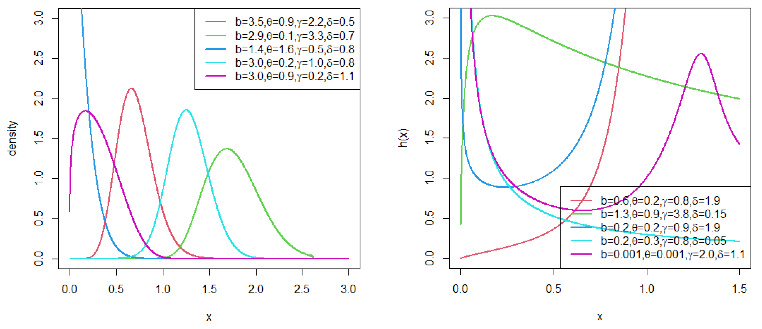
Figure 1 illustrates the plots for the PDF and HRF for the TL-HT-OBX-LLoG distribution. The PDF is highly flexible and can exhibit shapes ranging from right-skewed to left-skewed, nearly symmetric, or reverse-J. Similarly, the HRF can display various behaviors, including increasing, decreasing, bathtub, upside-down bathtub, or a combination of bathtub followed by upside-down bathtub patterns.

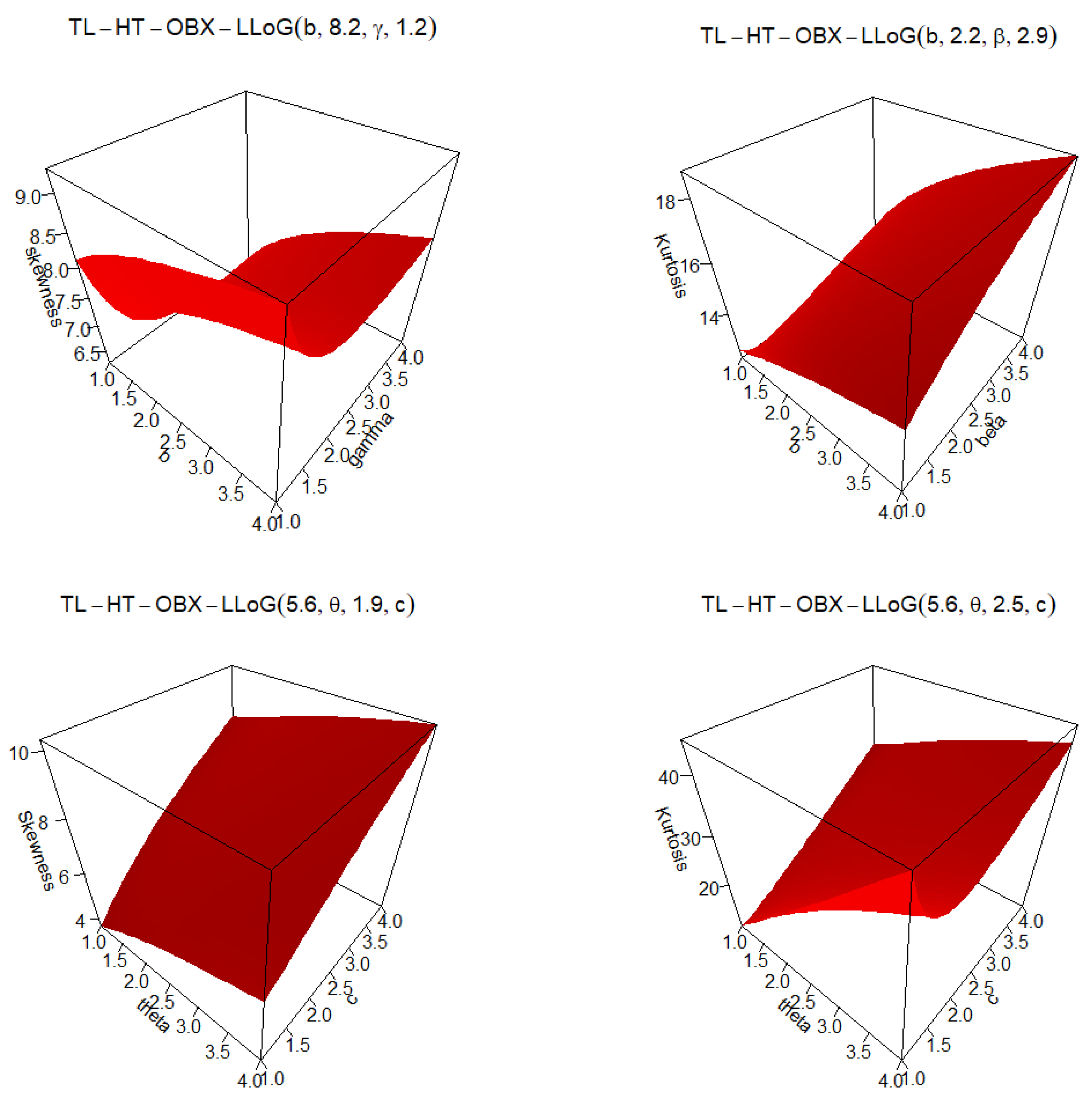
In Figure 2, the 3D graphs demonstrate the TL-HT-OBX-LLoG distribution in modelling data with various degrees of kurtosis (KT) and skewness(SK), highlighting its ability to model different complex real-world data patterns.

5.2. TL-HT-OBX-W Distribution

Considering the Weibull distribution as the baseline distribution, with its PDF and CDF defined as follows: $g(k;\delta )=\delta k^{\delta -1}exp(-k^{\delta })$ and $G(k;\delta )=1-exp(-k^{\delta })$, for $\delta >0$, then, the TL-HT-OBX-W CDF and pdPDF are defined as follows:

$$F_{TL-HT-OBX-W}(k;b,\theta ,\gamma ,\delta )={\left(1-{\left({\displaystyle \frac{1-F_{OBX-W}(k;\gamma ,\delta )}{1-(1-\theta )F_{OBX-W}(k;\gamma ,\delta )}}\right)}^{2\theta }\right)}^b$$

and

$$\begin{array}{ccc}\hfill f_{TL-HT-OBX-W}(k;b,\theta ,\gamma ,\delta )& =& 4b\gamma {\theta }^2{\displaystyle \frac{{\left(1-F_{OBX-W}(k;\gamma ,\delta )\right)}^{2\theta -1}}{{\left(1-(1-\theta )F_{OBX-W}(k;\gamma ,\delta )\right)}^{2\theta +1}}}\hfill \\ & \times & {\displaystyle \frac{\delta k^{\delta -1}exp(-x^{\delta })\left(1-exp(-k^{\delta })\right)}{exp(-3k^{\delta })}}\hfill \\ & \times & exp\left[-W_B(x;\delta )\right]F_{OBX-W}{(k;\gamma ,\delta )}^{-1}\hfill \\ & \times & {\left(1-{\left({\displaystyle \frac{1-F_{OBX-W}(k;\gamma ,\delta )}{1-(1-\theta )F_{OBX-W}(k;\gamma ,\delta )}}\right)}^{2\theta }\right)}^{b-1},\hfill \end{array}$$

respectively, for $b,\theta ,\gamma ,\delta >0,$ $k>0,$ where $F_{OBX-W}(k;\gamma ,\delta )={\left(1-exp\left[-{\left({\displaystyle \frac{1-exp(-k^{\delta })}{exp(-k^{\delta })}}\right)}^2\right]\right)}^{\gamma }$ and $W_B(x;\delta )=\left[-{\left({\displaystyle \frac{1-exp(-k^{\delta })}{exp(-k^{\delta })}}\right)}^2\right]$.

Figure 3 shows the PDF and hazard rate function(HRF) of the TL-HT-OBX-W distribution. The PDF exhibits considerable flexibility, taking forms such as nearly symmetric, left- or right-skewed, and reverse-J shape. Likewise, the HRF can assume a variety of patterns, including monotonically increasing or decreasing, bathtub-shaped, upside-down bathtub-shaped, or a combination of bathtub followed by upside-down bathtub behavior.

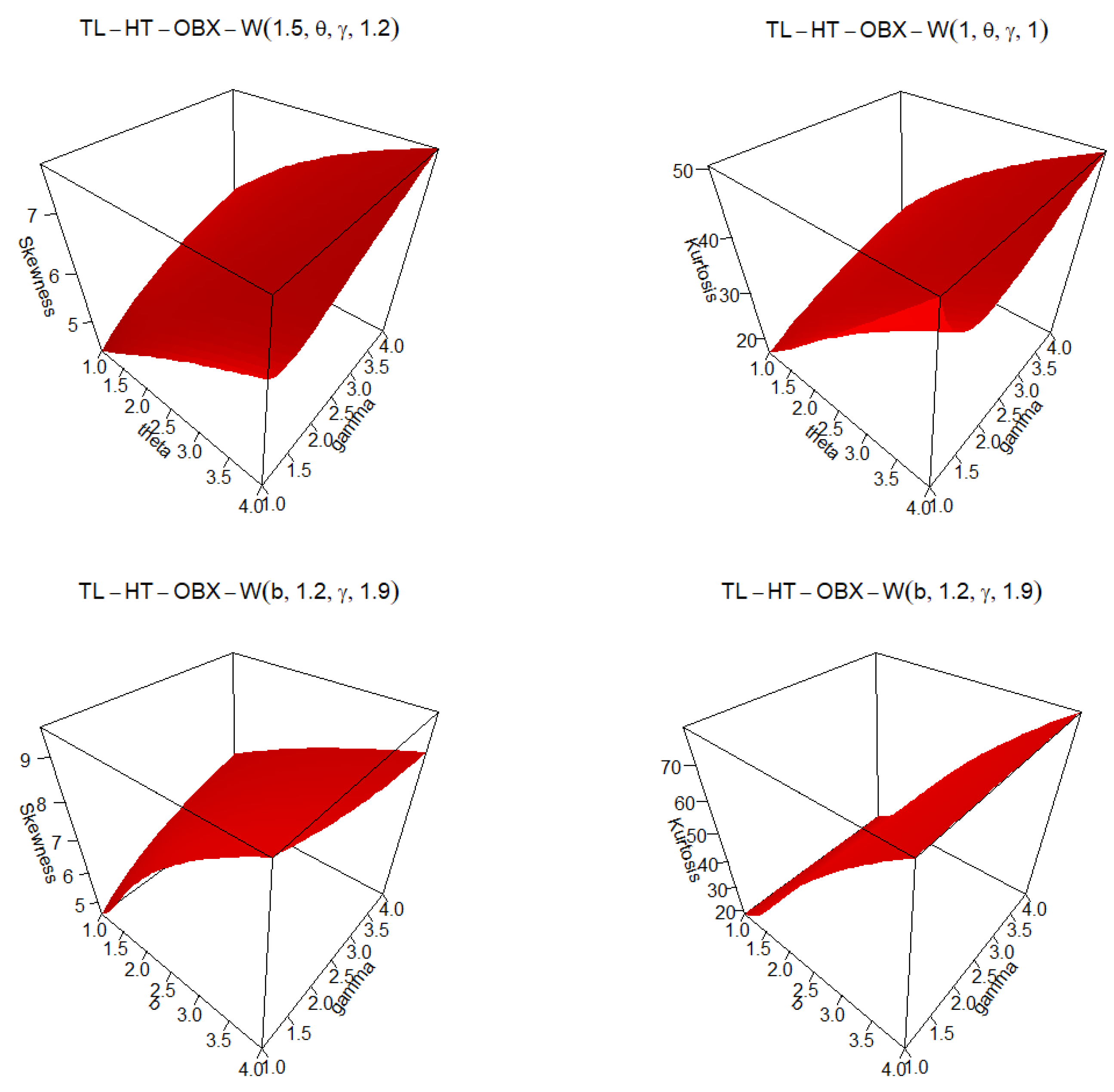
Figure 4 shows 3D plots of the TL-HT-OBX-W distribution capturing different levels of kurtosis and skewness. These graphs demonstrate its ability to represent complex real-world data.

5.3. TL-HT-OBX-Lx Distribution

Changing the parent distribution to the Lomax distribution PDF and CDF defined by $g(k;\alpha ,\beta )=\left({\displaystyle \frac{\alpha }{\beta }}\right){\left(1+{\displaystyle \frac{k}{\beta }}\right)}^{-\left(\alpha +1\right)}$ and $G(k;\alpha ,\beta )=1-{\left(1+{\displaystyle \frac{k}{\beta }}\right)}^{-\alpha }$, for $\alpha ,\beta >0$, respectively, we define the CDF and PDF of TL-HT-OBX-Lx distribution as follows:

$$\begin{array}{c}\hfill F_{TL-HT-OBX-L_X}(k;b,\theta ,\gamma ,\alpha ,\beta )={\left(1-{\left({\displaystyle \frac{1-F_{OBX-L_X}(k;\alpha ,\beta ,\gamma )}{1-(1-\theta )F_{OBX-L_X}(k;\alpha ,\beta ,\gamma )}}\right)}^{2\theta }\right)}^b\end{array}$$

(16)

and

$$\begin{array}{ccc}\hfill f_{TL-HT-OBX-L_X}(k;b,\theta ,\gamma ,\alpha ,\beta )& =& 4b\gamma {\theta }^2{\displaystyle \frac{{\left(1-F_{OBX-L_X}(k;\alpha ,\beta ,\gamma )\right)}^{2\theta -1}}{{\left(1-(1-\theta )F_{OBX-L_X}(k;\alpha ,\beta ,\gamma )\right)}^{2\theta +1}}}\hfill \\ & \times & {\displaystyle \frac{\left(\frac{\alpha }{\beta }\right){\left(1+\frac{k}{\beta }\right)}^{-\left(\alpha +1\right)}\left(1-{\left(1+\frac{k}{\beta }\right)}^{-\alpha }\right)}{{\left(1+\frac{k}{\beta }\right)}^{-3\alpha }}}\hfill \\ & \times & exp\left[-W_{L_X}(k;\alpha ,\beta )\right]{\left(1-exp\left[-K_{L_X}(k;\alpha ,\beta )\right]\right)}^{\gamma -1}\hfill \\ & \times & {\left(1-{\left({\displaystyle \frac{1-F_{OBX-L_X}(k;\alpha ,\beta ,\gamma )}{1-(1-\theta )F_{OBX-L_X}(k;\alpha ,\beta ,\gamma )}}\right)}^{2\theta }\right)}^{b-1},\hfill \end{array}$$

(17)

respectively, for $b,\theta ,\gamma ,\alpha ,\beta >0,$ $k>0,$ where $F_{OBX-L_X}(k;\alpha ,\beta ,\gamma )=$ ${\left(1-exp\left[-{\left({\displaystyle \frac{1-{\left(1+\frac{k}{\beta }\right)}^{-\alpha }}{{\left(1+\frac{k}{\beta }\right)}^{-\alpha }}}\right)}^2\right]\right)}^{\gamma }$ and $K_{L_X}(k;\alpha ,\beta )={\left({\displaystyle \frac{1-{\left(1+\frac{k}{\beta }\right)}^{-\alpha }}{{\left(1+\frac{k}{\beta }\right)}^{-\alpha }}}\right)}^2$

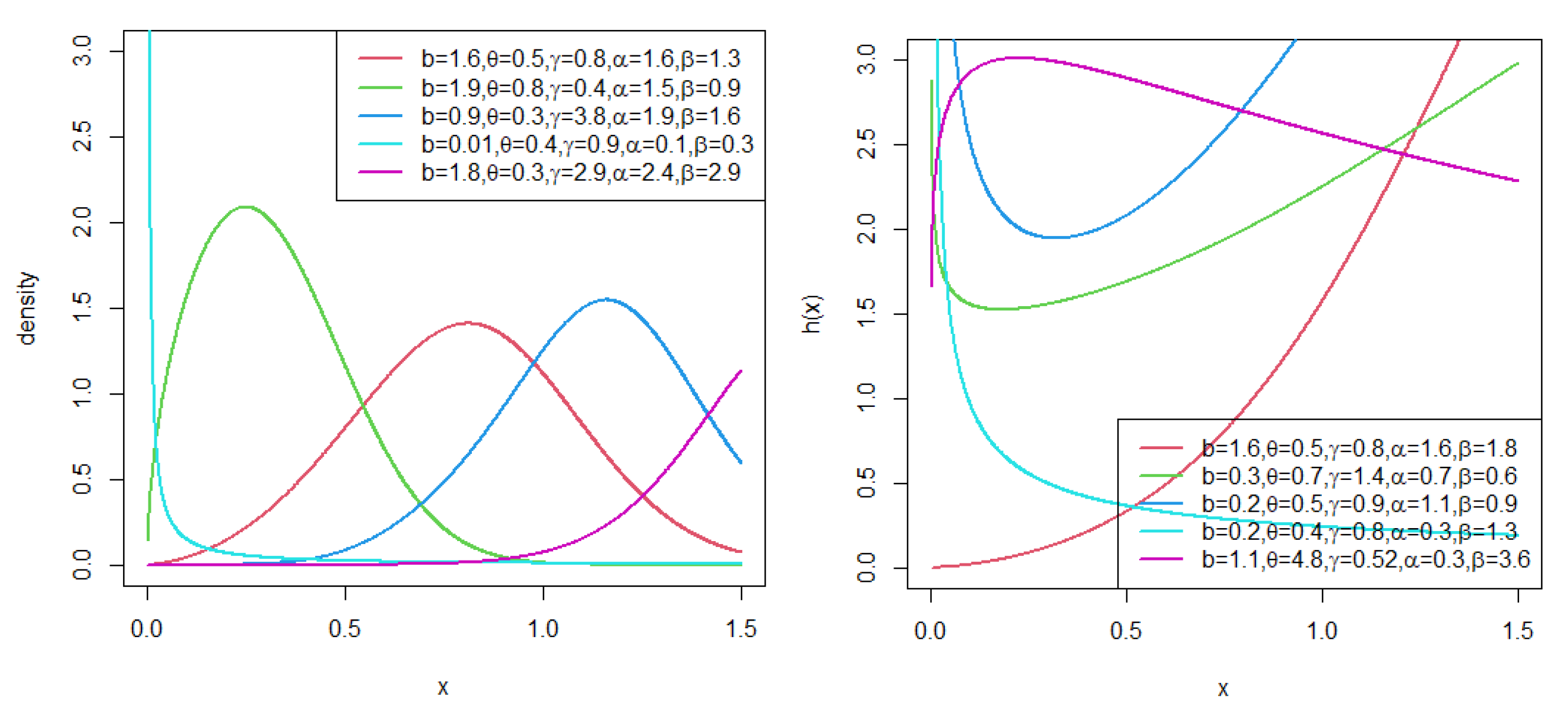
Figure 5 presents the PDF and HRF of the TL-HT-OBX-Lx distribution. The PDF demonstrates notable flexibility, accommodating a variety of shapes, including right-skewed, left-skewed, nearly symmetric, J-shaped, and reverse-J-shaped forms. Similarly, the HRF can exhibit multiple patterns, including monotonically decreasing or increasing, upside-down bathtub-shaped, or bathtub-shaped.

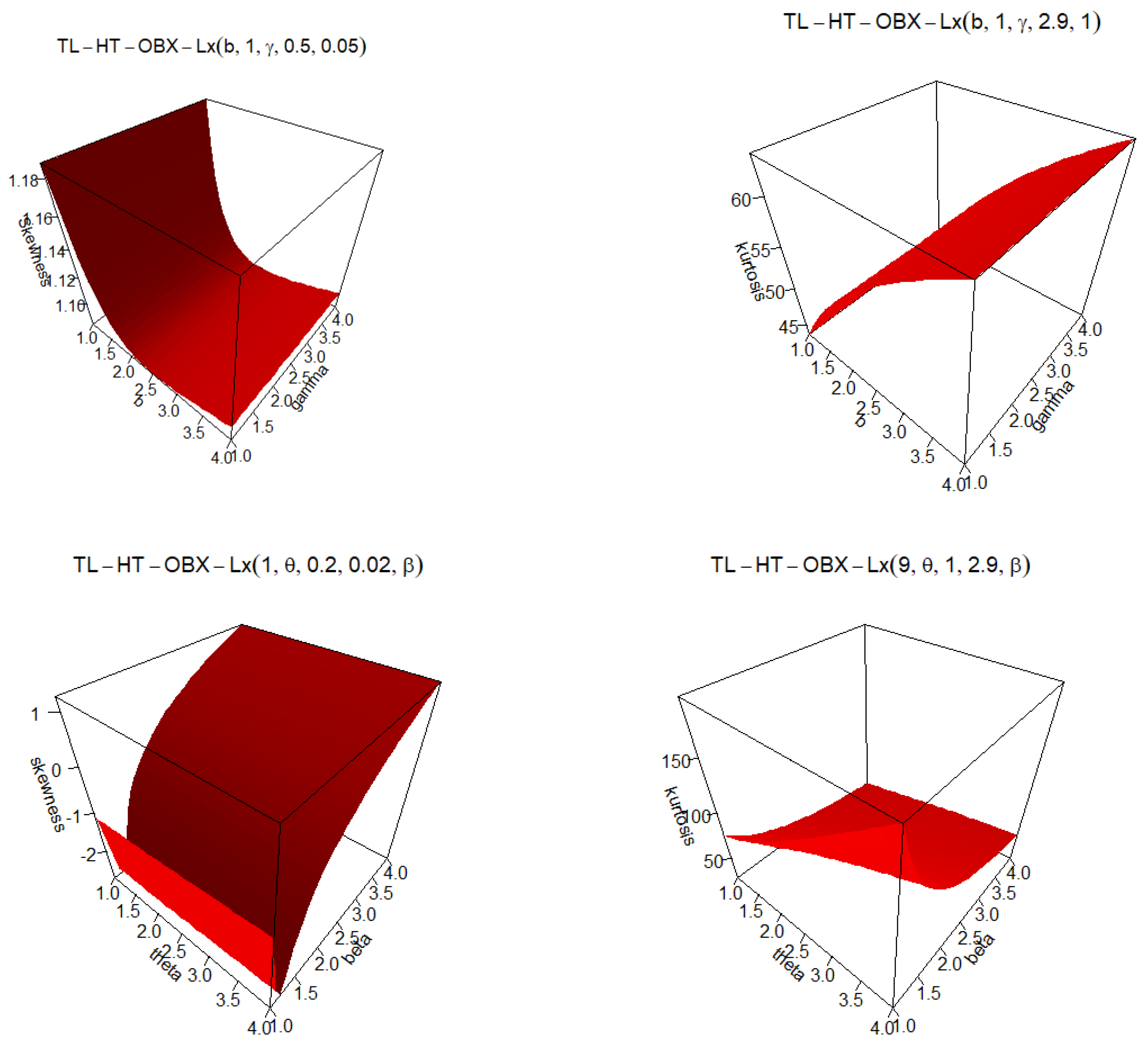
Figure 6 shows 3D plots of the TL-HT-OBX-Lx distribution capturing different levels of kurtosis and skewness.

6. Simulation Study

To evaluate the consistency of the parameter estimators for the TL-HT-OBX-LLoG distribution, we conducted simulation experiments using $N=3000$ on random samples of size $n=25,50,100,200,400,$ and 800. The root mean square errors (RMSEs) and average biases (ABias) corresponding to different estimation methods (MLE, OLSE, WLSE, RT-ADE, CVME, and ADE) are reported in

Table 1. Simulation results for $b=0.3, \theta =1.1, \gamma =0.7, c=1.9$.

		MLE		OLSE		WLSE		RT-ADE		CVME		ADE
n	Parameter	ABias	RMSE	ABias	RMSE	ABias	RMSE	ABias	RMSE	ABias	RMSE	ABias	RMSE
25	b	$1.{6009}^{\left\{1\right\}}$	$4.{7285}^{\left\{3\right\}}$	$-2.{1197}^{\left\{3\right\}}$	$3.{1217}^{\left\{2\right\}}$	$-1.{9966}^{\left\{2\right\}}$	$3.{0338}^{\left\{1\right\}}$	$3.{7873}^{\left\{6\right\}}$	$5.{3450}^{\left\{6\right\}}$	$-3.{1161}^{\left\{5\right\}}$	$5.{1184}^{\left\{5\right\}}$	$-2.{7403}^{\left\{4\right\}}$	$5.{0946}^{\left\{4\right\}}$
	$\theta$	$0.{3458}^{\left\{1\right\}}$	$1.{9755}^{\left\{1\right\}}$	$0.{9319}^{\left\{2\right\}}$	$2.{0095}^{\left\{4\right\}}$	$1.{8235}^{\left\{5\right\}}$	$2.{0139}^{\left\{5\right\}}$	$0.{9644}^{\left\{3\right\}}$	$1.{9961}^{\left\{2\right\}}$	$1.{9134}^{\left\{6\right\}}$	$2.{0093}^{\left\{3\right\}}$	$1.{8450}^{\left\{4\right\}}$	$2.{3108}^{\left\{6\right\}}$
	$\gamma$	$0.{1039}^{\left\{1\right\}}$	$0.{8184}^{\left\{1\right\}}$	$-0.{3899}^{\left\{6\right\}}$	$0.{9406}^{\left\{3\right\}}$	$-0.{1833}^{\left\{2\right\}}$	$0.{9247}^{\left\{2\right\}}$	$-0.{3723}^{\left\{4\right\}}$	$1.{1526}^{\left\{6\right\}}$	$-0.{3806}^{\left\{5\right\}}$	$0.{9564}^{\left\{4\right\}}$	$-0.{3454}^{\left\{3\right\}}$	$0.{9701}^{\left\{5\right\}}$
	c	$0.{1859}^{\left\{1\right\}}$	$1.{0416}^{\left\{1\right\}}$	$-0.{8625}^{\left\{4\right\}}$	$1.{2983}^{\left\{5\right\}}$	$-0.{4717}^{\left\{2\right\}}$	$1.{2148}^{\left\{4\right\}}$	$-1.{4976}^{\left\{6\right\}}$	$1.{5168}^{\left\{6\right\}}$	$-0.{7941}^{\left\{3\right\}}$	$1.{0907}^{\left\{2\right\}}$	$-1.{1410}^{\left\{5\right\}}$	$1.{1461}^{\left\{3\right\}}$
∑ ranks		10		27		23		39		33		34
50	b	$0.{7042}^{\left\{1\right\}}$	$1.{9371}^{\left\{1\right\}}$	$-1.{1192}^{\left\{3\right\}}$	$2.{2105}^{\left\{5\right\}}$	$1.{8508}^{\left\{4\right\}}$	$2.{0334}^{\left\{2\right\}}$	$2.{1719}^{\left\{6\right\}}$	$2.{3436}^{\left\{6\right\}}$	$-2.{1172}^{\left\{5\right\}}$	$2.{1187}^{\left\{4\right\}}$	$-1.{0696}^{\left\{2\right\}}$	$2.{0837}^{\left\{3\right\}}$
	$\theta$	$0.{1089}^{\left\{1\right\}}$	$0.{5718}^{\left\{1\right\}}$	$0.{8572}^{\left\{4\right\}}$	$0.{8819}^{\left\{3\right\}}$	$1.{0244}^{\left\{6\right\}}$	$1.{0460}^{\left\{5\right\}}$	$0.{6364}^{\left\{3\right\}}$	$1.{4963}^{\left\{5\right\}}$	$0.{8637}^{\left\{5\right\}}$	$0.{8898}^{\left\{4\right\}}$	$0.{6121}^{\left\{2\right\}}$	$0.{8293}^{\left\{2\right\}}$
	$\gamma$	$0.{0789}^{\left\{1\right\}}$	$0.{6643}^{\left\{1\right\}}$	$-0.{3377}^{\left\{4\right\}}$	$0.{7355}^{\left\{3\right\}}$	$-0.{1335}^{\left\{2\right\}}$	$0.{9221}^{\left\{5\right\}}$	$-0.{3260}^{\left\{3\right\}}$	$1.{1432}^{\left\{6\right\}}$	$-0.{3422}^{\left\{6\right\}}$	$0.{7036}^{\left\{2\right\}}$	$-0.{3421}^{\left\{5\right\}}$	$0.{7620}^{\left\{4\right\}}$
	c	$0.{0621}^{\left\{1\right\}}$	$0.{6399}^{\left\{1\right\}}$	$-0.{4698}^{\left\{3\right\}}$	$0.{8260}^{\left\{5\right\}}$	$-0.{4152}^{\left\{2\right\}}$	$0.{7115}^{\left\{4\right\}}$	$-1.{1003}^{\left\{6\right\}}$	$1.{2941}^{\left\{6\right\}}$	$-0.{5034}^{\left\{4\right\}}$	$0.{6413}^{\left\{2\right\}}$	$-0.{5913}^{\left\{5\right\}}$	$0.{6452}^{\left\{3\right\}}$
∑ ranks		8		30		30		41		32		26
100	b	$0.{5320}^{\left\{1\right\}}$	$1.{5018}^{\left\{1\right\}}$	$-1.{1178}^{\left\{4\right\}}$	$1.{8565}^{\left\{5\right\}}$	$1.{7848}^{\left\{6\right\}}$	$1.{8208}^{\left\{4\right\}}$	$1.{1787}^{\left\{5\right\}}$	$1.{6478}^{\left\{2\right\}}$	$-1.{1163}^{\left\{3\right\}}$	$2.{0171}^{\left\{6\right\}}$	$-0.{9569}^{\left\{2\right\}}$	$1.{6842}^{\left\{3\right\}}$
	$\theta$	$0.{0671}^{\left\{1\right\}}$	$0.{3494}^{\left\{1\right\}}$	$0.{5712}^{\left\{4\right\}}$	$0.{6888}^{\left\{4\right\}}$	$0.{6509}^{\left\{5\right\}}$	$0.{7243}^{\left\{5\right\}}$	$0.{2805}^{\left\{2\right\}}$	$0.{5239}^{\left\{3\right\}}$	$0.{6764}^{\left\{6\right\}}$	$0.{7885}^{\left\{6\right\}}$	$0.{4491}^{\left\{3\right\}}$	$0.{4640}^{\left\{2\right\}}$
	$\gamma$	$0.{0512}^{\left\{1\right\}}$	$0.{6076}^{\left\{2\right\}}$	$-0.{3126}^{\left\{5\right\}}$	$0.{7032}^{\left\{3\right\}}$	$-0.{0735}^{\left\{2\right\}}$	$0.{7166}^{\left\{4\right\}}$	$-0.{3065}^{\left\{4\right\}}$	$1.{1034}^{\left\{6\right\}}$	$-0.{3165}^{\left\{6\right\}}$	$0.{5831}^{\left\{1\right\}}$	$-0.{2409}^{\left\{3\right\}}$	$0.{7437}^{\left\{5\right\}}$
	c	$0.{0296}^{\left\{1\right\}}$	$0.{4861}^{\left\{1\right\}}$	$-0.{2271}^{\left\{2\right\}}$	$0.{5237}^{\left\{3\right\}}$	$-0.{3802}^{\left\{5\right\}}$	$0.{5124}^{\left\{2\right\}}$	$-1.{0713}^{\left\{6\right\}}$	$1.{2639}^{\left\{6\right\}}$	$-0.{2302}^{\left\{3\right\}}$	$0.{5241}^{\left\{4\right\}}$	$-0.{3061}^{\left\{4\right\}}$	$0.{5161}^{\left\{5\right\}}$
∑ ranks		9		30		33		34		35		27
200	b	$0.{1115}^{\left\{1\right\}}$	$0.{3314}^{\left\{1\right\}}$	$-0.{7799}^{\left\{5\right\}}$	$0.{8075}^{\left\{4\right\}}$	$0.{3266}^{\left\{2\right\}}$	$0.{4643}^{\left\{2\right\}}$	$0.{9046}^{\left\{6\right\}}$	$1.{3488}^{\left\{6\right\}}$	$-0.{7045}^{\left\{4\right\}}$	$0.{9117}^{\left\{5\right\}}$	$-0.{5308}^{\left\{3\right\}}$	$0.{6357}^{\left\{3\right\}}$
	$\theta$	$0.{0497}^{\left\{1\right\}}$	$0.{3254}^{\left\{1\right\}}$	$0.{3101}^{\left\{5\right\}}$	$0.{4102}^{\left\{3.5\right\}}$	$0.{5294}^{\left\{6\right\}}$	$0.{6428}^{\left\{6\right\}}$	$0.{2746}^{\left\{3\right\}}$	$0.{4560}^{\left\{5\right\}}$	$0.{3100}^{\left\{4\right\}}$	$0.{4102}^{\left\{3.5\right\}}$	$0.{2264}^{\left\{2\right\}}$	$0.{3590}^{\left\{2\right\}}$
	$\gamma$	$-0.{0299}^{\left\{1\right\}}$	$0.{4134}^{\left\{1\right\}}$	$-0.{3025}^{\left\{6\right\}}$	$0.{6307}^{\left\{6\right\}}$	$-0.{0679}^{\left\{2\right\}}$	$0.{4972}^{\left\{3\right\}}$	$-0.{2906}^{\left\{5\right\}}$	$0.{5254}^{\left\{4\right\}}$	$-0.{2033}^{\left\{4\right\}}$	$0.{4809}^{\left\{2\right\}}$	$-0.{1507}^{\left\{3\right\}}$	$0.{5269}^{\left\{5\right\}}$
	c	$0.{0240}^{\left\{1\right\}}$	$0.{2287}^{\left\{1\right\}}$	$-0.{1645}^{\left\{4\right\}}$	$0.{3220}^{\left\{3\right\}}$	$-0.{2685}^{\left\{5\right\}}$	$0.{3205}^{\left\{5\right\}}$	$-0.{8778}^{\left\{6\right\}}$	$1.{0534}^{\left\{6\right\}}$	$-0.{1721}^{\left\{3\right\}}$	$0.{3221}^{\left\{4\right\}}$	$-0.{3043}^{\left\{5\right\}}$	$0.{3082}^{\left\{2\right\}}$
∑ ranks		8		36.5		31		41		29.5		25
400	b	$0.{0301}^{\left\{1\right\}}$	$0.{1092}^{\left\{1\right\}}$	$-0.{5363}^{\left\{6\right\}}$	$0.{5448}^{\left\{5\right\}}$	$0.{3038}^{\left\{2\right\}}$	$0.{3565}^{\left\{2\right\}}$	$0.{5301}^{\left\{5\right\}}$	$0.{6445}^{\left\{6\right\}}$	$-0.{3804}^{\left\{4\right\}}$	$0.{5115}^{\left\{4\right\}}$	$-0.{3515}^{\left\{3\right\}}$	$0.{4522}^{\left\{3\right\}}$
	$\theta$	$0.{0039}^{\left\{1\right\}}$	$0.{1997}^{\left\{1\right\}}$	$0.{1486}^{\left\{3\right\}}$	$0.{2152}^{\left\{3\right\}}$	$0.{4436}^{\left\{6\right\}}$	$0.{5387}^{\left\{6\right\}}$	$0.{2685}^{\left\{5\right\}}$	$0.{3059}^{\left\{5\right\}}$	$0.{1485}^{\left\{2\right\}}$	$0.{2151}^{\left\{2\right\}}$	$0.{2039}^{\left\{4\right\}}$	$0.{2406}^{\left\{4\right\}}$
	$\gamma$	$-0.{0116}^{\left\{1\right\}}$	$0.{1432}^{\left\{1\right\}}$	$-0.{1344}^{\left\{4\right\}}$	$0.{2347}^{\left\{2\right\}}$	$-0.{0517}^{\left\{3\right\}}$	$0.{2662}^{\left\{5\right\}}$	$-0.{2749}^{\left\{3\right\}}$	$0.{3968}^{\left\{6\right\}}$	$-0.{1345}^{\left\{5\right\}}$	$0.{2348}^{\left\{3\right\}}$	$-0.{0516}^{\left\{2\right\}}$	$0.{2522}^{\left\{4\right\}}$
	c	$0.{0205}^{\left\{1\right\}}$	$0.{1582}^{\left\{1\right\}}$	$-0.{1023}^{\left\{2\right\}}$	$0.{2410}^{\left\{3\right\}}$	$-0.{1767}^{\left\{4\right\}}$	$0.{2888}^{\left\{5\right\}}$	$-0.{4567}^{\left\{6\right\}}$	$0.{4723}^{\left\{6\right\}}$	$-0.{1024}^{\left\{3\right\}}$	$0.{2411}^{\left\{4\right\}}$	$-0.{2096}^{\left\{5\right\}}$	$0.{2310}^{\left\{2\right\}}$
∑ ranks		8		28		33		42		27		27
800	b	$0.{0152}^{\left\{1\right\}}$	$0.{0543}^{\left\{1\right\}}$	$-0.{2132}^{\left\{5\right\}}$	$0.{3324}^{\left\{5\right\}}$	$0.{1587}^{\left\{4\right\}}$	$0.{2187}^{\left\{4\right\}}$	$0.{2700}^{\left\{6\right\}}$	$0.{3538}^{\left\{6\right\}}$	$-0.{1132}^{\left\{2\right\}}$	$0.{2133}^{\left\{3\right\}}$	$-0.{1505}^{\left\{3\right\}}$	$0.{1706}^{\left\{2\right\}}$
	$\theta$	$-0.{0001}^{\left\{1\right\}}$	$0.{1149}^{\left\{1\right\}}$	$0.{1091}^{\left\{2\right\}}$	$0.{1920}^{\left\{3\right\}}$	$0.{2712}^{\left\{6\right\}}$	$0.{3713}^{\left\{6\right\}}$	$0.{1593}^{\left\{5\right\}}$	$0.{2063}^{\left\{5\right\}}$	$0.{1176}^{\left\{3\right\}}$	$0.{1921}^{\left\{4\right\}}$	$0.{1452}^{\left\{4\right\}}$	$0.{1655}^{\left\{2\right\}}$
	$\gamma$	$-0.{0089}^{\left\{1\right\}}$	$0.{1015}^{\left\{1\right\}}$	$-0.{0854}^{\left\{4\right\}}$	$0.{1386}^{\left\{2\right\}}$	$-0.{0378}^{\left\{3\right\}}$	$0.{1414}^{\left\{4\right\}}$	$-0.{1710}^{\left\{6\right\}}$	$0.{2174}^{\left\{6\right\}}$	$-0.{0855}^{\left\{5\right\}}$	$0.{1387}^{\left\{3\right\}}$	$-0.{0325}^{\left\{2\right\}}$	$0.{1570}^{\left\{5\right\}}$
	c	$-0.{0021}^{\left\{1\right\}}$	$0.{1027}^{\left\{1\right\}}$	$-0.{0652}^{\left\{2\right\}}$	$0.{1265}^{\left\{2\right\}}$	$-0.{0825}^{\left\{4\right\}}$	$0.{2260}^{\left\{5\right\}}$	$-0.{2855}^{\left\{6\right\}}$	$0.{3411}^{\left\{6\right\}}$	$-0.{0653}^{\left\{3\right\}}$	$0.{1657}^{\left\{3\right\}}$	$-0.{1067}^{\left\{5\right\}}$	$0.{2069}^{\left\{4\right\}}$
∑ ranks		8		25		35		44		27		29

and

Table 2. Simulation results for $b=2.0, \theta =0.9, \gamma =0.9, c=0.5$.

		MLE		OLSE		WLSE		RT-ADE		CVME		ADE
n	Parameter	ABias	RMSE	ABias	RMSE	ABias	RMSE	ABias	RMSE	ABias	RMSE	ABias	RMSE
25	b	$0.{1481}^{\left\{1\right\}}$	$0.{4053}^{\left\{2\right\}}$	$-0.{2260}^{\left\{3\right\}}$	$0.{3152}^{\left\{1\right\}}$	$-1.{0461}^{\left\{6\right\}}$	$1.{0566}^{\left\{5\right\}}$	$0.{9915}^{\left\{5\right\}}$	$1.{9439}^{\left\{6\right\}}$	$-0.{2085}^{\left\{2\right\}}$	$0.{5010}^{\left\{3\right\}}$	$-0.{3247}^{\left\{4\right\}}$	$0.{7408}^{\left\{4\right\}}$
	$\theta$	$0.{4466}^{\left\{1\right\}}$	$1.{3981}^{\left\{1\right\}}$	$0.{8274}^{\left\{5\right\}}$	$1.{9163}^{\left\{6\right\}}$	$0.{7990}^{\left\{4\right\}}$	$1.{7972}^{\left\{5\right\}}$	$0.{7604}^{\left\{3\right\}}$	$1.{7829}^{\left\{4\right\}}$	$0.{7065}^{\left\{2\right\}}$	$1.{4055}^{\left\{2\right\}}$	$1.{5217}^{\left\{6\right\}}$	$1.{6495}^{\left\{3\right\}}$
	$\gamma$	$0.{1235}^{\left\{1\right\}}$	$0.{8280}^{\left\{1\right\}}$	$1.{1005}^{\left\{5\right\}}$	$1.{1108}^{\left\{4\right\}}$	$1.{0229}^{\left\{3\right\}}$	$1.{2837}^{\left\{5\right\}}$	$1.{0361}^{\left\{4\right\}}$	$1.{0947}^{\left\{2\right\}}$	$0.{9477}^{\left\{2\right\}}$	$1.{1051}^{\left\{3\right\}}$	$1.{1284}^{\left\{6\right\}}$	$1.{1353}^{\left\{6\right\}}$
	c	$0.{3071}^{\left\{2\right\}}$	$0.{9507}^{\left\{1\right\}}$	$-0.{8023}^{\left\{5\right\}}$	$1.{1110}^{\left\{3\right\}}$	$-0.{5710}^{\left\{4\right\}}$	$1.{0692}^{\left\{2\right\}}$	$-0.{5049}^{\left\{3\right\}}$	$1.{4531}^{\left\{5\right\}}$	$-0.{8559}^{\left\{6\right\}}$	$1.{1431}^{\left\{4\right\}}$	$-0.{1440}^{\left\{1\right\}}$	$1.{4654}^{\left\{6\right\}}$
∑ ranks		10		32		34		32		24		36
50	b	$0.{1197}^{\left\{1\right\}}$	$0.{2988}^{\left\{1\right\}}$	$-0.{1953}^{\left\{3\right\}}$	$0.{3018}^{\left\{2\right\}}$	$-0.{3025}^{\left\{5\right\}}$	$0.{9007}^{\left\{5\right\}}$	$0.{8605}^{\left\{6\right\}}$	$1.{1252}^{\left\{6\right\}}$	$-0.{1805}^{\left\{2\right\}}$	$0.{3676}^{\left\{3\right\}}$	$-0.{2516}^{\left\{4\right\}}$	$0.{5683}^{\left\{4\right\}}$
	$\theta$	$0.{2913}^{\left\{1\right\}}$	$1.{1914}^{\left\{1\right\}}$	$0.{7759}^{\left\{5\right\}}$	$1.{2113}^{\left\{3\right\}}$	$0.{6080}^{\left\{2\right\}}$	$1.{3091}^{\left\{4\right\}}$	$0.{7559}^{\left\{4\right\}}$	$1.{7129}^{\left\{6\right\}}$	$0.{6788}^{\left\{3\right\}}$	$1.{2016}^{\left\{2\right\}}$	$1.{5115}^{\left\{6\right\}}$	$1.{6000}^{\left\{5\right\}}$
	$\gamma$	$0.{0904}^{\left\{2\right\}}$	$0.{5004}^{\left\{1\right\}}$	$0.{8034}^{\left\{4\right\}}$	$0.{9149}^{\left\{4\right\}}$	$0.{3271}^{\left\{1\right\}}$	$0.{6703}^{\left\{3\right\}}$	$0.{9548}^{\left\{5\right\}}$	$0.{9892}^{\left\{6\right\}}$	$0.{5992}^{\left\{3\right\}}$	$0.{6105}^{\left\{2\right\}}$	$1.{0254}^{\left\{6\right\}}$	$0.{9303}^{\left\{5\right\}}$
	c	$0.{2140}^{\left\{1\right\}}$	$0.{6356}^{\left\{1\right\}}$	$-0.{5831}^{\left\{5\right\}}$	$0.{7157}^{\left\{2\right\}}$	$-0.{4167}^{\left\{2\right\}}$	$0.{7650}^{\left\{4\right\}}$	$-0.{4676}^{\left\{4\right\}}$	$0.{7857}^{\left\{5\right\}}$	$-0.{6889}^{\left\{6\right\}}$	$0.{9183}^{\left\{6\right\}}$	$-0.{4387}^{\left\{3\right\}}$	$0.{7400}^{\left\{3\right\}}$
∑ ranks		9		28		26		42		27		36
100	b	$0.{0810}^{\left\{1\right\}}$	$0.{2058}^{\left\{1\right\}}$	$-0.{1397}^{\left\{3\right\}}$	$0.{2099}^{\left\{2\right\}}$	$-0.{2512}^{\left\{5\right\}}$	$0.{4902}^{\left\{5\right\}}$	$0.{6709}^{\left\{6\right\}}$	$0.{8351}^{\left\{6\right\}}$	$-0.{1329}^{\left\{2\right\}}$	$0.{2605}^{\left\{4\right\}}$	$-0.{1535}^{\left\{4\right\}}$	$0.{2547}^{\left\{3\right\}}$
	$\theta$	$0.{2834}^{\left\{1\right\}}$	$1.{1513}^{\left\{2\right\}}$	$0.{6870}^{\left\{5\right\}}$	$1.{2012}^{\left\{4\right\}}$	$-0.{5131}^{\left\{2\right\}}$	$1.{2516}^{\left\{6\right\}}$	$0.{5905}^{\left\{3\right\}}$	$1.{0971}^{\left\{1\right\}}$	$0.{6226}^{\left\{4\right\}}$	$1.{1944}^{\left\{3\right\}}$	$1.{1551}^{\left\{6\right\}}$	$1.{2048}^{\left\{5\right\}}$
	$\gamma$	$0.{0764}^{\left\{1\right\}}$	$0.{4677}^{\left\{1\right\}}$	$0.{4321}^{\left\{5\right\}}$	$0.{6302}^{\left\{5\right\}}$	$-0.{2171}^{\left\{2\right\}}$	$0.{5875}^{\left\{4\right\}}$	$0.{2908}^{\left\{3\right\}}$	$0.{5425}^{\left\{3\right\}}$	$0.{3109}^{\left\{4\right\}}$	$0.{5129}^{\left\{2\right\}}$	$0.{6967}^{\left\{6\right\}}$	$0.{7301}^{\left\{6\right\}}$
	c	$0.{1949}^{\left\{1\right\}}$	$0.{5843}^{\left\{1\right\}}$	$-0.{3966}^{\left\{4\right\}}$	$0.{6214}^{\left\{2\right\}}$	$0.{2988}^{\left\{2\right\}}$	$0.{6984}^{\left\{6\right\}}$	$-0.{4579}^{\left\{5\right\}}$	$0.{6875}^{\left\{5\right\}}$	$-0.{5003}^{\left\{6\right\}}$	$0.{6231}^{\left\{3\right\}}$	$-0.{3603}^{\left\{3\right\}}$	$0.{6366}^{\left\{4\right\}}$
∑ ranks		9		28		26		42		27		36
200	b	$0.{0512}^{\left\{1\right\}}$	$0.{1418}^{\left\{1\right\}}$	$-0.{0886}^{\left\{3\right\}}$	$0.{1835}^{\left\{2\right\}}$	$-0.{1747}^{\left\{5\right\}}$	$0.{2299}^{\left\{5\right\}}$	$0.{2310}^{\left\{6\right\}}$	$0.{3859}^{\left\{6\right\}}$	$-0.{0867}^{\left\{2\right\}}$	$0.{1919}^{\left\{3\right\}}$	$-0.{1248}^{\left\{4\right\}}$	$0.{2086}^{\left\{4\right\}}$
	$\theta$	$0.{2383}^{\left\{1\right\}}$	$0.{9602}^{\left\{1\right\}}$	$0.{5859}^{\left\{6\right\}}$	$1.{0882}^{\left\{5\right\}}$	$0.{3091}^{\left\{2\right\}}$	$1.{0268}^{\left\{4\right\}}$	$0.{3101}^{\left\{3\right\}}$	$1.{0027}^{\left\{2\right\}}$	$0.{5474}^{\left\{5\right\}}$	$1.{0083}^{\left\{3\right\}}$	$0.{5101}^{\left\{4\right\}}$	$1.{1544}^{\left\{6\right\}}$
	$\gamma$	$0.{0756}^{\left\{1\right\}}$	$0.{3863}^{\left\{1\right\}}$	$0.{3657}^{\left\{5\right\}}$	$0.{4102}^{\left\{3\right\}}$	$-0.{1013}^{\left\{2\right\}}$	$0.{4598}^{\left\{6\right\}}$	$0.{2795}^{\left\{3\right\}}$	$0.{4268}^{\left\{4\right\}}$	$0.{2953}^{\left\{4\right\}}$	$0.{4087}^{\left\{2\right\}}$	$0.{3808}^{\left\{6\right\}}$	$0.{4398}^{\left\{5\right\}}$
	c	$0.{0910}^{\left\{1\right\}}$	$0.{3899}^{\left\{1\right\}}$	$-0.{1126}^{\left\{2\right\}}$	$0.{4793}^{\left\{4\right\}}$	$0.{1558}^{\left\{5\right\}}$	$0.{4928}^{\left\{6\right\}}$	$-0.{3899}^{\left\{6\right\}}$	$0.{4899}^{\left\{5\right\}}$	$-0.{1426}^{\left\{4\right\}}$	$0.{4257}^{\left\{3\right\}}$	$-0.{1335}^{\left\{3\right\}}$	$0.{3954}^{\left\{2\right\}}$
∑ ranks		8		30		32		32		28		37
400	b	$0.{0258}^{\left\{1\right\}}$	$0.{0934}^{\left\{2\right\}}$	$-0.{0782}^{\left\{3\right\}}$	$0.{0983}^{\left\{3\right\}}$	$-0.{1226}^{\left\{5\right\}}$	$0.{1561}^{\left\{4\right\}}$	$0.{1325}^{\left\{6\right\}}$	$0.{2015}^{\left\{6\right\}}$	$-0.{0774}^{\left\{2\right\}}$	$0.{0884}^{\left\{1\right\}}$	$-0.{1080}^{\left\{4\right\}}$	$0.{1857}^{\left\{5\right\}}$
	$\theta$	$0.{1932}^{\left\{3\right\}}$	$0.{8666}^{\left\{2\right\}}$	$0.{1436}^{\left\{1\right\}}$	$0.{9681}^{\left\{6\right\}}$	$0.{2156}^{\left\{4\right\}}$	$0.{9169}^{\left\{4\right\}}$	$0.{1758}^{\left\{2\right\}}$	$0.{9053}^{\left\{3\right\}}$	$0.{4144}^{\left\{6\right\}}$	$0.{9656}^{\left\{5\right\}}$	$0.{3285}^{\left\{5\right\}}$	$0.{7713}^{\left\{1\right\}}$
	$\gamma$	$0.{0674}^{\left\{1\right\}}$	$0.{3727}^{\left\{2\right\}}$	$0.{2092}^{\left\{5\right\}}$	$0.{4036}^{\left\{5\right\}}$	$-0.{0855}^{\left\{2\right\}}$	$0.{3636}^{\left\{1\right\}}$	$0.{1964}^{\left\{4\right\}}$	$0.{4058}^{\left\{6\right\}}$	$0.{1046}^{\left\{3\right\}}$	$0.{4002}^{\left\{3\right\}}$	$0.{2105}^{\left\{6\right\}}$	$0.{4011}^{\left\{4\right\}}$
	c	$0.{0478}^{\left\{1\right\}}$	$0.{2837}^{\left\{2\right\}}$	$-0.{1021}^{\left\{3\right\}}$	$0.{3075}^{\left\{3\right\}}$	$0.{1039}^{\left\{4\right\}}$	$0.{3917}^{\left\{6\right\}}$	$-0.{1899}^{\left\{6\right\}}$	$0.{3899}^{\left\{5\right\}}$	$-0.{0774}^{\left\{2\right\}}$	$0.{0884}^{\left\{1\right\}}$	$-0.{1080}^{\left\{5\right\}}$	$0.{3080}^{\left\{4\right\}}$
∑ ranks		14		29		30		38		23		34
800	b	$0.{0118}^{\left\{1\right\}}$	$0.{0617}^{\left\{1\right\}}$	$-0.{0734}^{\left\{6\right\}}$	$0.{0785}^{\left\{4\right\}}$	$-0.{0513}^{\left\{5\right\}}$	$0.{0737}^{\left\{2\right\}}$	$0.{0474}^{\left\{4\right\}}$	$0.{1027}^{\left\{5\right\}}$	$-0.{0305}^{\left\{2\right\}}$	$0.{0780}^{\left\{3\right\}}$	$-0.{0316}^{\left\{3\right\}}$	$0.{1066}^{\left\{6\right\}}$
	$\theta$	$0.{0606}^{\left\{1\right\}}$	$0.{3980}^{\left\{1\right\}}$	$0.{1150}^{\left\{4\right\}}$	$0.{4280}^{\left\{3\right\}}$	$0.{1685}^{\left\{5\right\}}$	$0.{4725}^{\left\{4\right\}}$	$0.{0995}^{\left\{2\right\}}$	$0.{5967}^{\left\{6\right\}}$	$0.{1138}^{\left\{3\right\}}$	$0.{4266}^{\left\{2\right\}}$	$0.{1777}^{\left\{6\right\}}$	$0.{4803}^{\left\{5\right\}}$
	$\gamma$	$0.{0452}^{\left\{1\right\}}$	$0.{3050}^{\left\{1\right\}}$	$0.{0768}^{\left\{3\right\}}$	$0.{3081}^{\left\{2\right\}}$	$-0.{0775}^{\left\{4\right\}}$	$0.{3508}^{\left\{4\right\}}$	$0.{1277}^{\left\{6\right\}}$	$0.{3823}^{\left\{6\right\}}$	$0.{0765}^{\left\{2\right\}}$	$0.{3814}^{\left\{5\right\}}$	$0.{1225}^{\left\{5\right\}}$	$0.{3236}^{\left\{3\right\}}$
	c	$0.{0253}^{\left\{1\right\}}$	$0.{1968}^{\left\{1\right\}}$	$-0.{0378}^{\left\{2\right\}}$	$0.{2414}^{\left\{3\right\}}$	$0.{0922}^{\left\{4\right\}}$	$0.{2764}^{\left\{5\right\}}$	$-0.{0899}^{\left\{3\right\}}$	$0.{2899}^{\left\{6\right\}}$	$-0.{1082}^{\left\{6\right\}}$	$0.{2418}^{\left\{4\right\}}$	$-0.{0954}^{\left\{5\right\}}$	$0.{2094}^{\left\{2\right\}}$
∑ ranks		8		27		33		38		27		35

. For a given parameter, say $\theta$, the ABias and RMSE are calculated using the following expressions:

$$ABias\left(\widehat{\theta }\right)={\displaystyle \frac{1}{N}}\sum _{i=1}^N{\widehat{\theta }}_i-\theta ,\mathrm{and}RMSE\left(\widehat{\theta }\right)=\sqrt{{\displaystyle \frac{1}{N}}\sum _{i=1}^N{({\widehat{\theta }}_i-\theta )}^2}.$$

The inversion sampling technique is applied via numerical CDF using the following steps:

•

compute the CDF numerically using R algorithm;

•

invert it using interpolation using R algorithm.

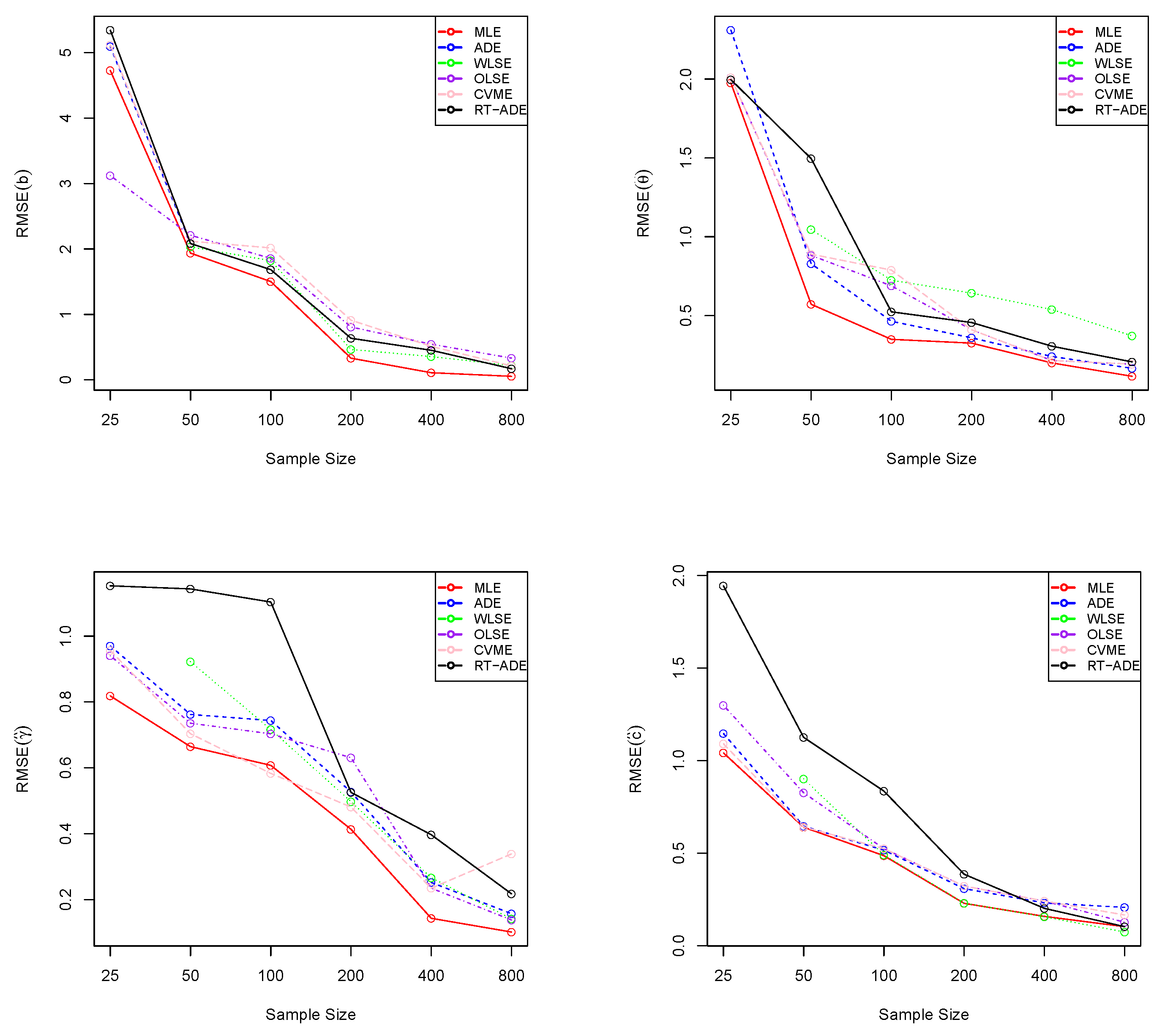
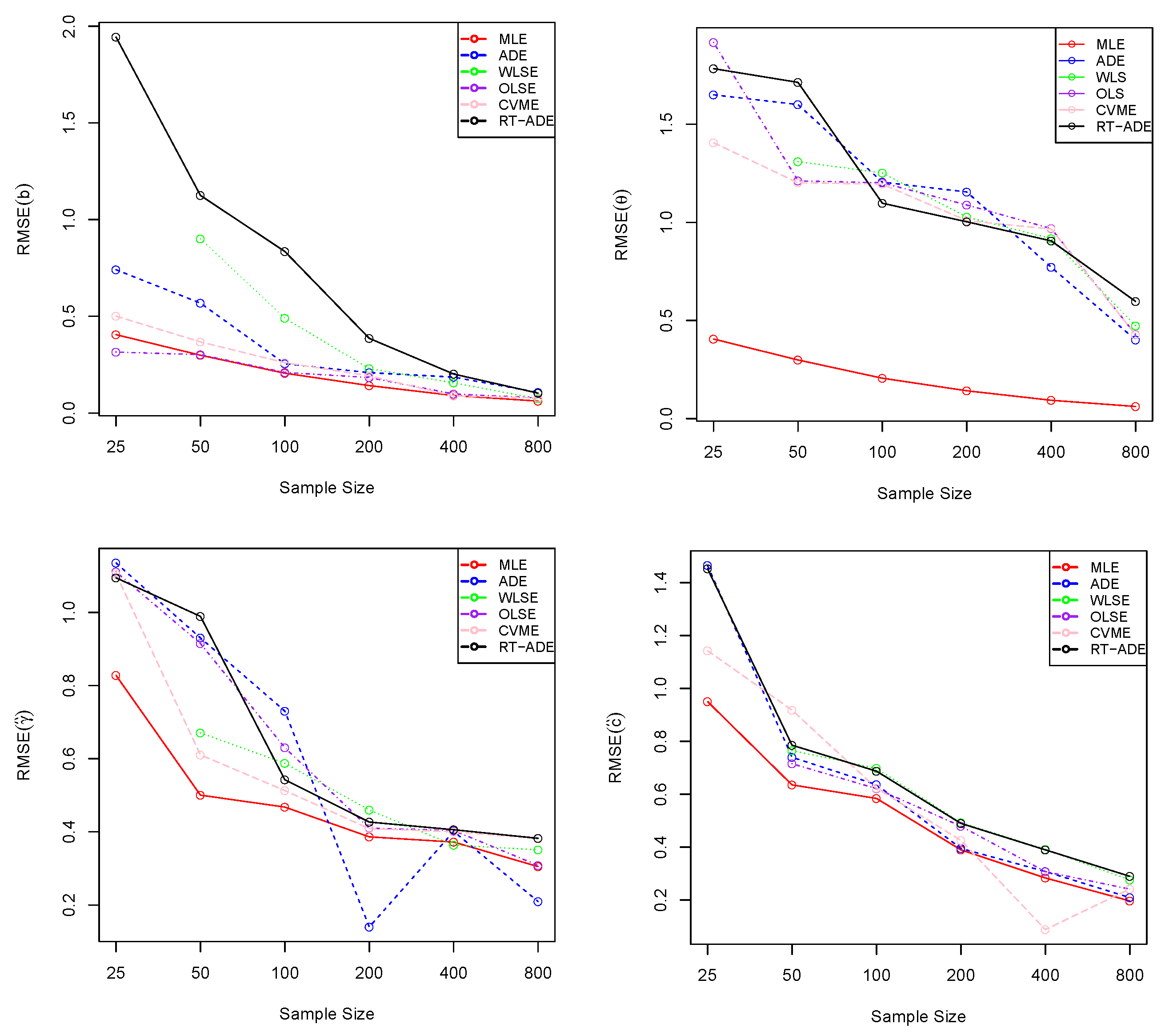
Table 1 and Table 2 show the ABias and RMSE and partial ranks as superscripts for each estimation techniques. Sum of ranks is given

Table 3. Partial and overall ranks.

Parameters	n	MLE	OLSE	WLSE	RT-ADE	CVME	ADE
$b=0.3, \theta =1.1, \gamma =0.7, c=1.9$	25	1.0	3.0	2.0	6.0	4.0	5.0
	50	1.0	3.5	3.5	6.0	5.0	2.0
	100	1.0	3.0	4.0	5.0	6.0	2.0
	200	1.0	5.0	4.0	6.0	3.0	2.0
	400	1.0	4.0	5.0	6.0	2.5	2.5
	800	1.0	2.0	5.0	6.0	3.0	4.0
$b=2.0, \theta =0.9, \gamma =0.9, c=0.5$	25	1.0	3.5	5.0	3.5	2.0	6.0
	50	1.0	4.0	2.0	6.0	3.0	5.0
	100	1.0	4.0	2.0	6.0	3.0	5.0
	200	1.0	3.0	4.5	4.5	2.0	6.0
	400	1.0	3.0	4.0	6.0	2.0	5.0
	800	1.0	2.5	4.0	6.0	2.5	5.0
Sum of Ranks ($\mathrm{\Sigma }$ ranks)		12.0	40.5	45	67.0	38.0	49.5
Overall Rank		1	3	4	6	2	5

with the MLE method ranking first for a given metric. Figure 7 and Figure 8 illustrate the effectiveness of different estimation methods with decreasing ABias and RMSE for increasing sample size. MLE stands out as the most reliable method for larger sample sizes, followed by CVME and OLSE. The other methods (RT-ADE, WLSE, ADE) maintain moderate RMSE.

7. Actuarial Risk Measures

Several actuarial risk metrics including Value at Risk (VaR), Tail Variance (TV), Tail Value at Risk (TVaR), and Tail Variance Premium (TVP) are considered in this section.

7.1. VaR

VaR is a widely used actuarial measure for evaluating financial market risk. Also referred to as the quantile risk measure or the quantile premium principle, VaR is defined at a predetermined confidence level, typically 90%, 95%, or 99%. For the TL-HT-OBX-G FOD, VaR can be calculated using the following expression:

$$X_p=G^{-1}\left[{\left({\left[-log\left(1-{\left[{\displaystyle \frac{1-{\left(1-p^{\frac{1}{b}}\right)}^{\frac{1}{2\theta }}}{1-\left(1-\theta \right){\left(1-p^{\frac{1}{b}}\right)}^{\frac{1}{2\theta }}}}\right]}^{{\displaystyle \frac{1}{\gamma }}}\right)\right]}^{{\displaystyle \frac{-1}{2}}}+1\right)}^{-1}\right]$$

where p is the specified significance level within the interval (0, 1).

7.2. TVaR

TVaR is another key actuarial measure frequently employed to quantify risk. It represents the expected loss given that an outcome exceeds a specified probability threshold. For the TL-HT-OBX-G FOD, TVaR, known as the Conditional Tail Expectation (CTE) or Tail Conditional Expectation (TCE), can be expressed as follows:

$$\begin{array}{ccc}\hfill {\mathrm{TVaR}}_p& =& E(K\mid K>k_p)={\displaystyle \frac{1}{1-p}}{\int }_{Va{R}_p}^{\infty }kf\left(k\right)dk\hfill \\ & =& {\displaystyle \frac{1}{1-p}}\sum _{q=0}^{\infty }{\int }_{Va{R}_p}^{\infty }k{\omega }_{q+1}{g}_{q+1}(k;\nu )dk,\hfill \end{array}$$

(18)

where ${\omega }_{q+1}$ is defined by Equation (8).

7.3. TV

TV is a crucial actuarial measure that examines the variance beyond VaR. TV for the TL-HT-OBX-G FoD is given by the following:

$$\begin{array}{ccc}\hfill T{V}_p& =& E(K^2\mid K>k_p)-{\left(TVa{R}_p\right)}^2\hfill \\ & =& {\displaystyle \frac{1}{1-p}}{\int }_{Va{R}_p}^{\infty }{k}^{2}f\left(k\right)dk-{\left(TVa{R}_p\right)}^2\hfill \\ & =& {\displaystyle \frac{1}{1-p}}\sum _{q=0}^{\infty }{\omega }_{q+1}{\int }_{Va{R}_p}^{\infty }{k}^2{g}_{q+1}(k;\nu )dk-{\left(TVa{R}_p\right)}^2,\hfill \end{array}$$

(19)

where $g_{q+1}(k;\nu )=(q+1){\left[G(k;\nu )\right]}^{q}g(k;\nu )$ represents the Exp-G pdf and ${\omega }_{q+1}$ is given by Equation (8). Therefore, the TV of the TL-HT-OBX-G FOD may be directly derived from the TV of the Exp-G distribution.

7.4. TVP

TVP is a vital actuarial measure with significant applications in insurance sciences. For the TL-HT-OBX-G FOD, TVP is defined as follows:

$$TV{P}_p=TVa{R}_p+\delta \left(T{V}_p\right),$$

(20)

where $0<\delta <1$. The TVP for this FOD is determined by substituting the results from Equations (18) and (19) into the above equation.

7.5. Numerical Investigation of Actuarial Risk Measures

This subsection presents numerical simulations for the actuarial risk metrics, including Value at Risk (VaR), Tail Risk Expectation (TRE, formerly TVaR), Tail Variance (TV), and Tail Variance Premium (TVP). The performance of the TL-HT-OBX-G distribution was assessed relative to its sub-models to examine the impact of additional parameters on tail behavior. Comparisons were also conducted with non-nested models, specifically the Topp–Leone odd Burr III–log-logistic (TL-OBIII-LLoG) distribution Moakofi et al. [13] and the Alpha-Power Extended Log-Logistic (APExLLD) distribution Teamah et al. [5]. The simulation procedure was implemented as follows:

• Random samples of size $n=100$ were generated from each distribution, with parameters estimated via the ML estimation method.
• A total of 1000 repetitions were conducted to compute the VaR, TRE, TV, and TVP for all distributions.

Table 4. Simulation results of VaR, TVaR, TV and TVP.

Significance Level		0.7	0.75	0.8	0.85	0.9	0.95
TL-HT-OBX-LLoG ($b=1.9, \theta =0.6, \gamma =2.9, c=0.9$)	VaR	1.0900	1.1243	1.1629	1.2084	1.2667	1.3550
	TVaR	2.5753	2.8945	3.3405	4.0218	5.2357	8.2734
	TV	6.7601	9.0587	12.9110	20.3024	38.2684	112.9639
	TVP	2.1567	3.8995	6.9882	13.2352	29.2059	99.0422
TL-HT-OBX-LLoG ($\theta =0.6, \gamma =2.9, c=0.9$)	VaR	0.9820	1.0197	1.0614	1.1097	1.1701	1.2587
	TVaR	2.2263	2.4837	2.8363	3.3611	4.2620	6.3805
	TV	2.2452	3.1552	4.6563	7.4590	13.9535	38.5016
	TVP	0.6546	0.7173	0.8887	2.9790	8.2961	30.1960
TL-HT-OBX-LLoG ($b=1.9, \theta =0.6, c=0.9$)	VaR	0.8637	0.9097	0.9614	1.0223	1.0998	1.2160
	TVaR	1.1192	1.1643	1.2178	1.2845	1.3754	1.5235
	TV	0.0394	0.0606	0.0899	0.1341	0.2109	0.3908
	TVP	1.0916	1.1188	1.1458	1.1705	1.1856	1.1922
TL-HT-OBX-LLoG ($\theta =0.6, c=0.9$)	VaR	0.7146	0.7752	0.8446	0.9280	1.0365	1.2036
	TVaR	1.5786	1.7425	1.9563	2.2540	2.7154	3.5995
	TV	0.6999	0.9981	1.4591	2.2374	3.7630	7.7935
	TVP	0.7892	0.9939	0.7890	0.3522	0.6712	3.8042
TL-HT-OBX-LLoG ($b=1.9, c=0.9$)	VaR	0.9318	0.9879	1.0522	1.1295	1.2303	1.3866
	TVaR	1.1440	1.1809	1.2213	1.2653	1.3093	1.3178
	TV	0.0662	0.0711	0.0806	0.0992	0.1410	0.2664
	TVP	1.1903	1.2343	1.2858	1.3497	1.4363	1.5709
APExLLD ($\alpha =0.9, a=4.9, b=0.2, c=0.9$)	VaR	0.2286	0.2406	0.2550	0.2736	0.3002	0.3489
	TVaR	0.2989	0.3118	0.3278	0.3491	0.3807	0.4401
	TV	0.0076	0.0081	0.0088	0.0098	0.0116	0.0155
	TVP	0.3042	0.3179	0.3349	0.3575	0.3912	0.4549
TL-OBIII-LLoG ($\alpha =1.9, \beta =0.6, b=2.9, \lambda =0.9$)	VaR	0.0188	0.0244	0.0321	0.0432	0.0610	0.0960
	TVaR	0.0188	0.0244	0.3212	0.0432	0.0616	0.0960
	TV	0.0026	0.0027	0.0029	0.0031	0.0033	0.0035
	TVP	0.0632	0.07146	0. 0820	0.0964	0.1180	0.1573

summarizes the numerical results for VaR, TRE, TV, and TVP across the compared distributions. Higher values of these measures indicate heavier-tailed behavior for the corresponding model.

8. Applications

The TL-HT-OBX-LLoG distribution is applied to three real-world datasets to demonstrate its practical utility. Model performance is evaluated using the AdequacyModel package in R. The TL-HT-OBX-LLoG distribution is compared with some non-nested models through a range of goodness-of-fit metrics, including the negative twice log-likelihood statistic $(-2ln(L\left)\right)$, Akaike Information Criterion ($AIC=2p-2ln\left(L\right)$), Bayesian Information Criterion ($BIC=pln\left(n\right)-2ln\left(L\right)$), and the consistent AIC ($AICC=AIC+2{\displaystyle \frac{p(p+1)}{n-p-1}}$), where $L=L\left(\widehat{\Delta }\right)$ denotes the likelihood function evaluated at the estimated parameters, n is the sample size, and p is the number of estimated parameters. Additional goodness-of-fit statistics considered include the Cramér–von Mises statistic ($W^{*}$), Anderson–Darling statistic ($A^{*}$), the Kolmogorov–Smirnov (K–S) statistic, along with its associated p-value, and the Sum of Squares (SS) from probability plots. The Cramér–von Mises and Anderson–Darling statistics are described in Chen and Balakrishnan [14]. The SS from probability plots is computed as follows:

$$SS=\sum _{j=1}^n{\left[F\left(k_{\left(j\right)}\right)-{\displaystyle \frac{j-0.375}{n+0.25}}\right]}^2,$$

where $j=1,2,\dots ,n$ and $k_{\left(j\right)}$ represents the ordered observations [15]. A model exhibiting the smallest values of these goodness-of-fit statistics and the highest p-value from the K–S test is considered the best fitting model for the given dataset.

The non-nested models we used for comparison include: Topp–Leone Marshall–Olkin–Weibull (TL-MO-W) distribution by Chipepa et al. [16], Topp–Leone generated Weibull (TLGW) distribution by Aryal et al. [17], Topp–Leone Odd Burr III–log-logistic (TL-OBIII-LLoG) distribution by Moakofi et al. [13], Ristić -Balakhrishman–Topp–Leone–Gompertz–log-logistic (RB-TL-Gom-LLoG) distribution by Pu et al. [18], and the APExLLD distribution by Teamah et al. [5].

8.1. European COVID-19 Data

This data, sourced from the [World Health Organization COVID-19 dashboard] (https://covid19.who.int/, accessed on 12 August 2025 ), shows daily COVID-19 death counts in Europe.

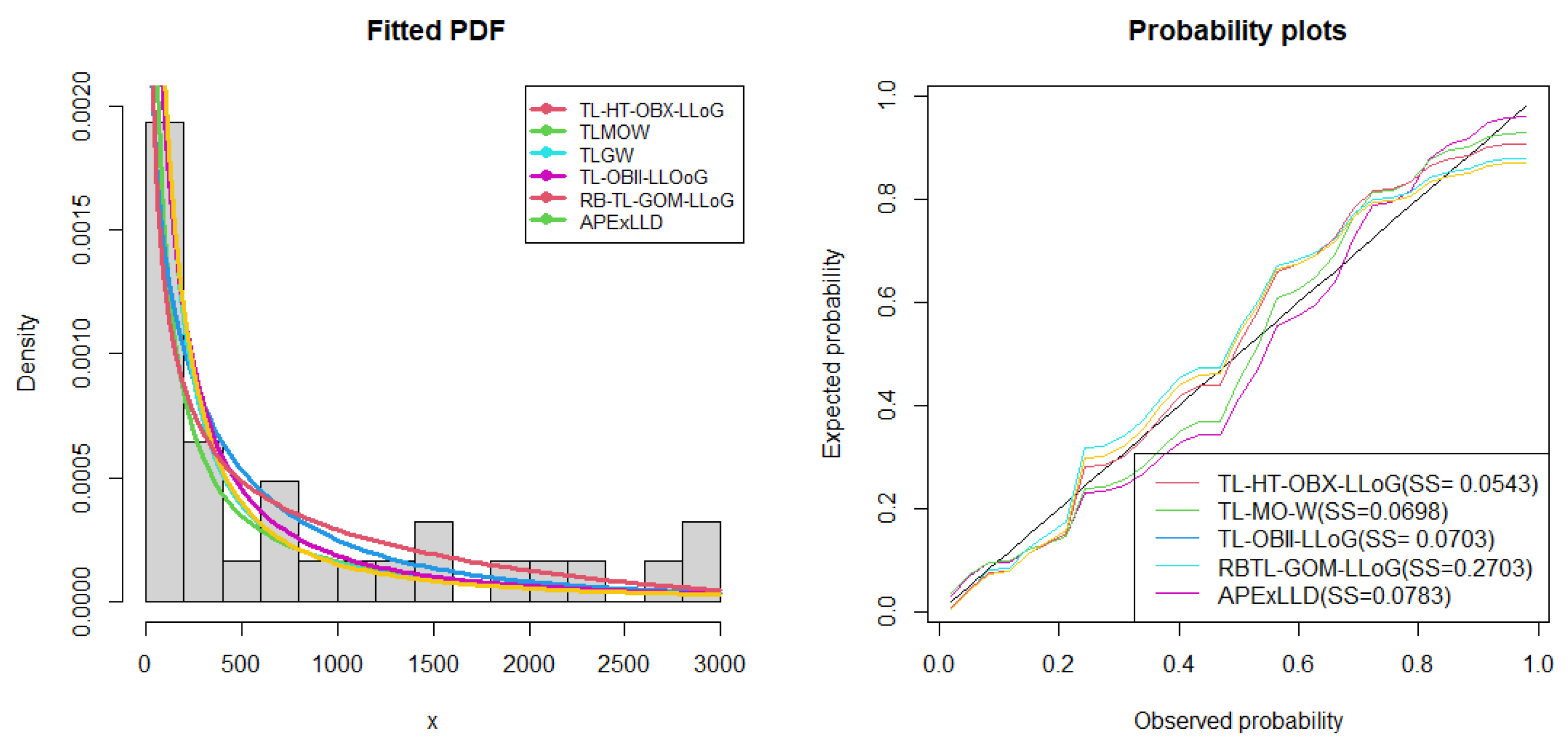
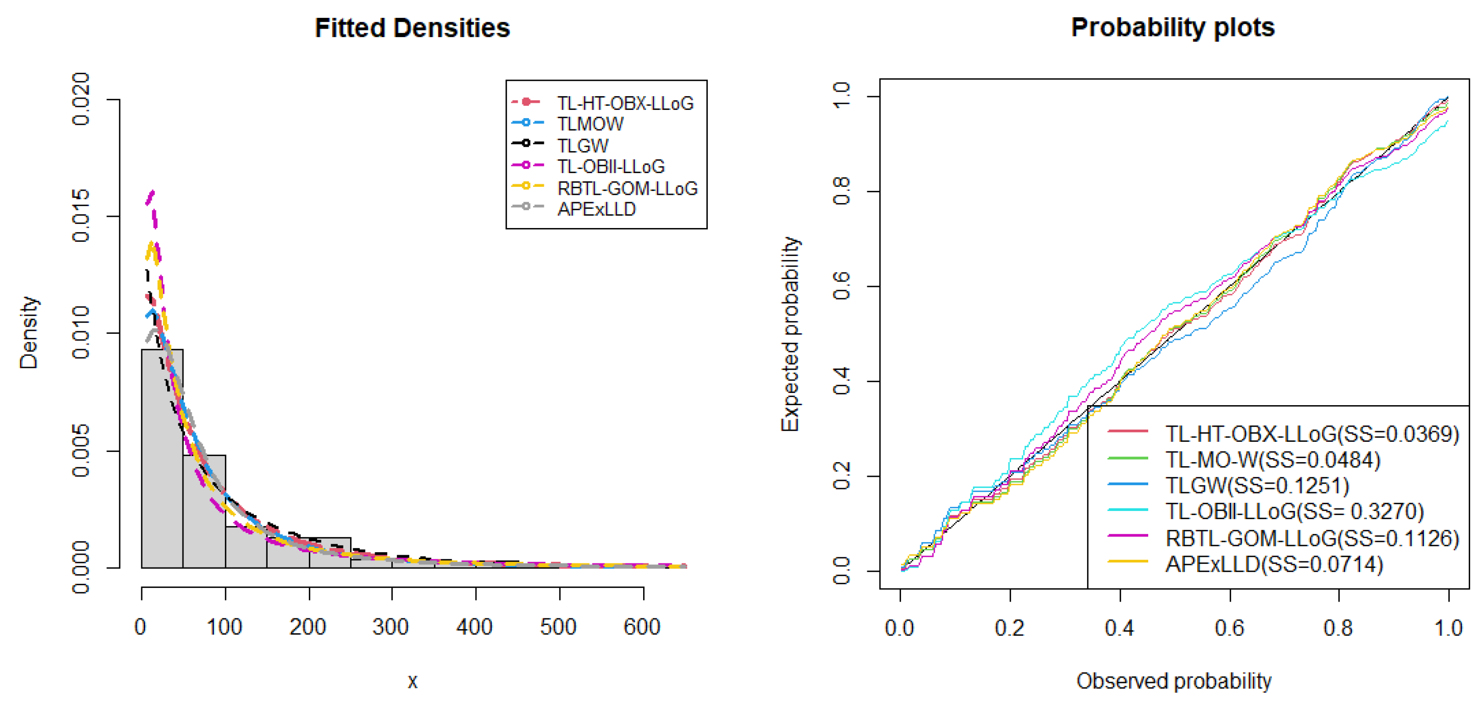
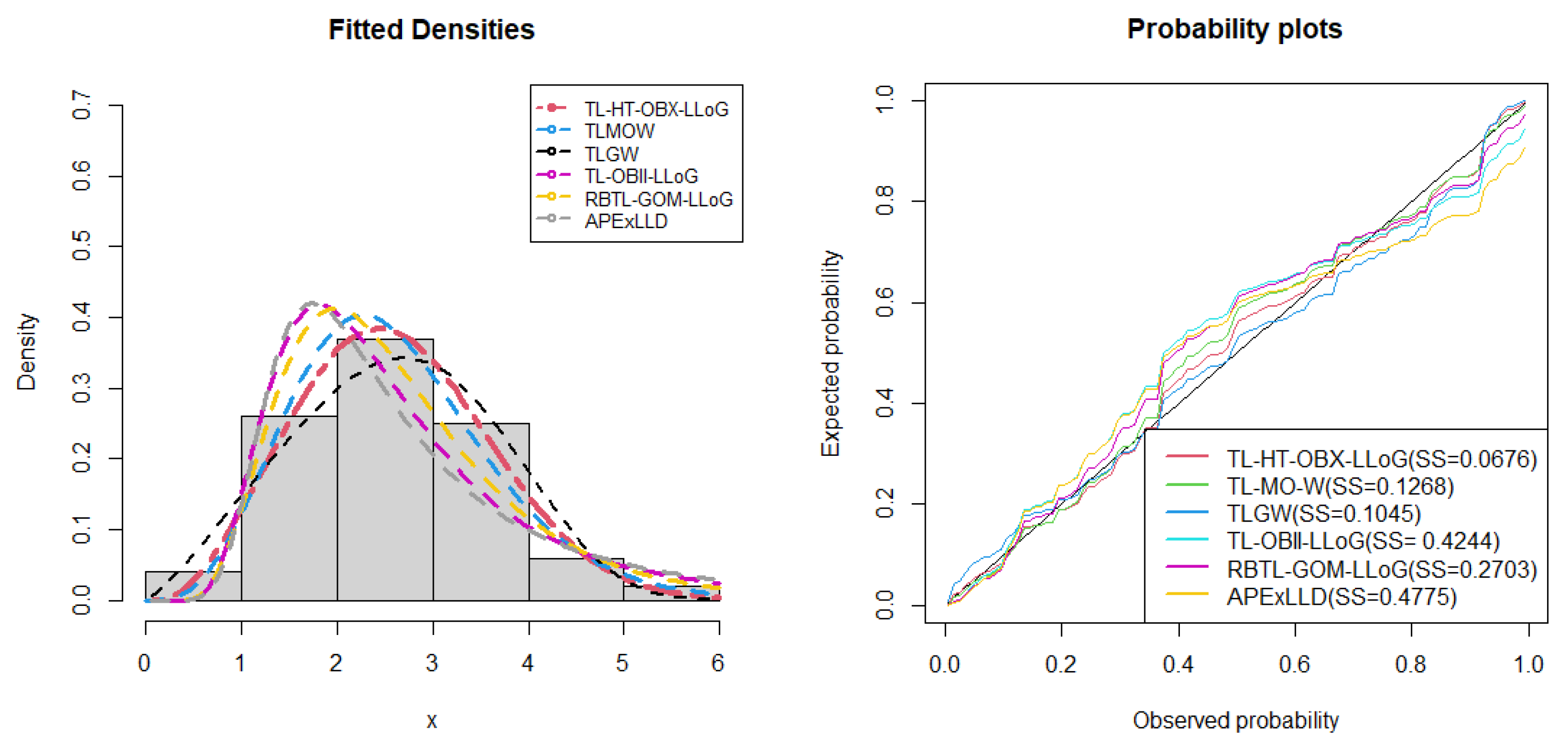
For the European COVID-19 dataset, the TL-HT-OBX-LLoG distribution demonstrated superior performance compared to the non-nested models, as illustrated in

Table 5. MLEs and goodness-of-fit statistics for European COVID-19 data.

	Estimates				Statistics
Model	$\mathit{b}$	$\mathit{\theta }$	$\mathit{\gamma }$	$\mathit{c}$	$-\mathbf{2}log\mathit{L}$	$\mathit{AIC}$	$\mathit{AICC}$	$\mathit{BIC}$	${\mathit{W}}^{*}$	${\mathit{A}}^{*}$	K-S	p-Value
TL-HT-OBX-LLoG	0.1632	77.0570	86.2790	0.0527	469.8573	477.8573	479.3958	483.5933	0.0612	0.4063	0.1395	0.8363
	(0.0309)	($1.7772\times {10}^{-6}$)	($7.3147\times {10}^{-5}$)	(0.0012)
	b	$\delta$	$\gamma$	$\lambda$
TL-MO-W	1.4593	0.8235	$1.0292\times {10}^{+7}$	0.0644	474.6477	482.6477	484.1862	488.3836	0.0743	0.5126	0.1137	0.7756
	($7.8111\times {10}^{-1}$ )	($2.5195\times {10}^{-7}$ )	($3.7905\times {10}^{-2}$ )	(3.3077)
	$\alpha$	$\theta$	$\lambda$	$\beta$
TLGW	2.1406	1.0016	0.0009	0.3249	479.6846	487.6843	489.2227	493.4202	0.0594	0.432755	0.1381	0.5492
	(0.6769)	(0.2702 )	(0.0007 )	(0.0627)
	$\alpha$	$\beta$	b	$\lambda$
TL-OBIII-LLoG	23.6880	54.3560	0.3035	0.0218	477.9591	485.9591	487.4976	491.6951	0.0944	0.6608	0.1213	0.7065
	($1.7886\times {10}^{-6}$)	(0.0004)	(0.0838)	(0.0019)
	$\delta$	b	$\alpha$	c
RBTL-GOM-LLoG	117.5400	639.1300	0.2550	0.03700	474.9944	482.9944	484.5328	488.7303	0.0684	0.4988	0.11157	0.7949
	($7.7912\times {10}^{-4}$)	($1.6696\times {10}^{-4}$)	($6.4888\times {10}^{-2}$)	($5.7681\times {10}^{-3}$)
	$\alpha$	a	b	c
APExLLD	17.7183	0.7336	2.9073	7.3059	478.9729	486.9729	488.5116	492.7088	0.1020	0.7046	0.1306	0.6188
	(49.5295)	(0.1981)	(31.6092)	(47.4060)

. The TL-HT-OBX-LLoG distribution yielded the lowest goodness-of-fit statistic and the highest p-value for the K–S test, indicating it is the most suitable model for this dataset. The TL-HT-OBX-LLoG distribution provided a better fit for the European COVID-19 data compared to the non-nested models, as shown in Figure 9.

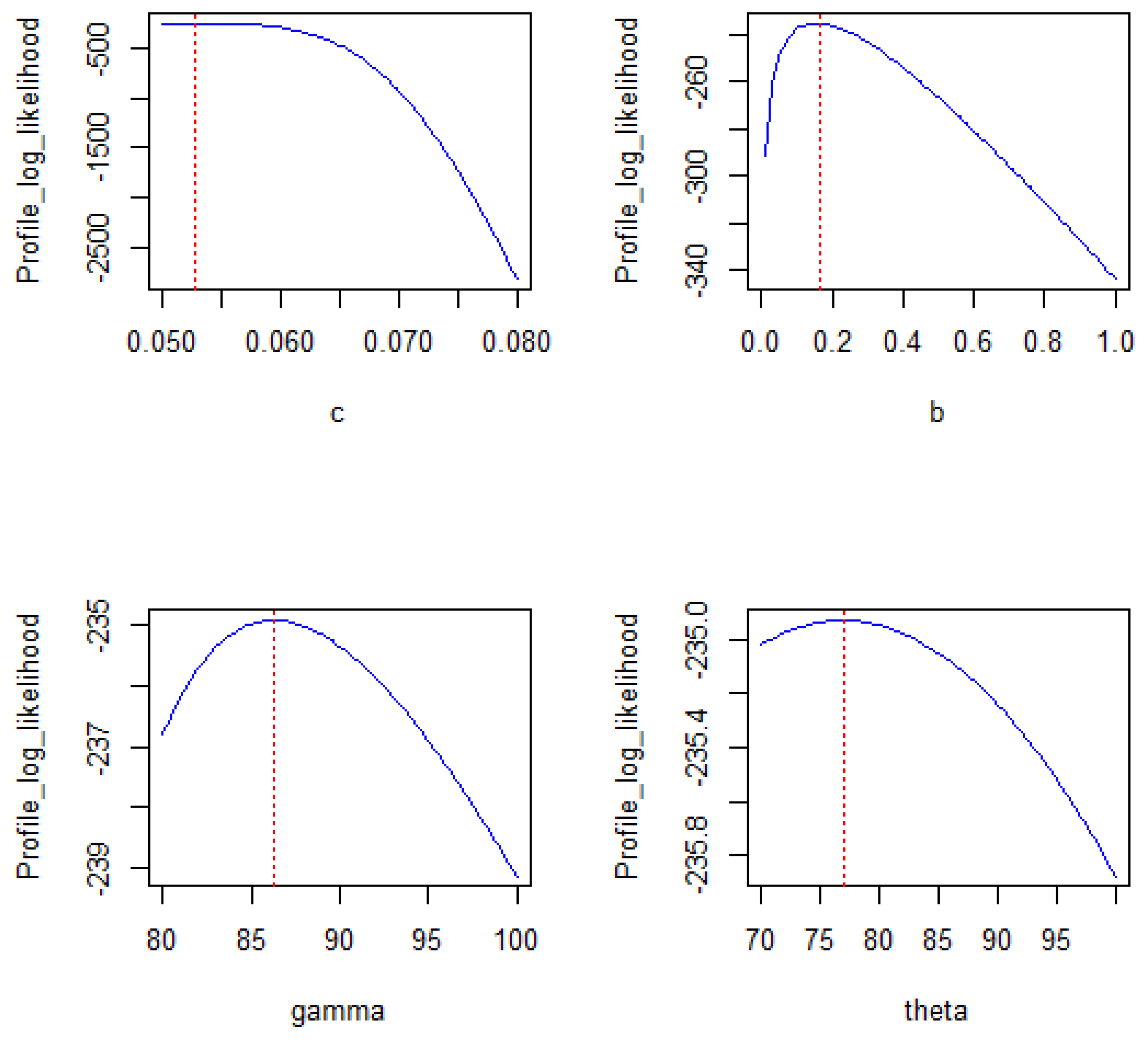
In Figure 10, we observe that the MLEs for the TL-HT-OBX-LLoG distribution are achieved uniquely. Figure 11 displays the Kaplan–Meier (K-M) survival curve, empirical cdf (ECDF), scaled total time on test (TTT) transform plot, and fitted HRF for the European COVID-19 data. The fitted model aligns well with both the ECDF and the K-M curve, and the scaled TTT transform plot reveals a bathtub-shaped HRF which is correctly depicted by the TL-HT-OBX-LLoG model.

8.2. Air Conditioning System Data

The second dataset was recently analyzed by Muhammad and Yahaya [19] represents the number of successive failures obtained from the air conditioning system of each member in a fleet of 13 Boeing 720 jet air-planes.

The TL-HT-OBX-LLoG distribution outperformed the non-nested models as shown in

Table 6. MLEs and goodness-of-fit statistics for air conditioning system data.

	Estimates				Statistics
Model	$\mathit{b}$	$\mathit{\theta }$	$\mathit{\gamma }$	$\mathit{c}$	$-\mathbf{2}log\left(\mathit{L}\right)$	$\mathit{AIC}$	$\mathit{AICC}$	$\mathit{BIC}$	${\mathit{W}}^{*}$	${\mathit{A}}^{*}$	K-S	p-Value
TL-HT-OBX-LLoG	1.9239	93.3560	27.1493	0.0240	2349.263	2357.263	2357.456	2370.708	0.0361	0.2664	0.0389	0.9032
	(0.9029)	(0.0942)	(2.3284)	(0.0042)
	b	$\delta$	$\gamma$	$\lambda$
TL-MO-W	1.4593	$2.2656\times {10}^{06}$	$7.1962\times {10}^{-02}$	10.621	2353.468	2361.468	2361.661	2374.913	0.0532	0.4013	0.0424	0.8380
	($4.1863\times {10}^{-01}$ )	($2.5930\times {10}^{-07}$ )	($1.0072\times {10}^{-02}$ )	($6.6382\times {10}^{-01}$)
	$\alpha$	$\theta$	$\lambda$	$\beta$
TLGW	$6.2227\times {10}^{01}$	$1.5161\times {10}^{-02}$	$1.8468\times {10}^{-03}$	3.3233	2351.21	2359.209	2359.402	2372.654	0.0933	0.5971	0.0604	0.4188
	($1.6335\times {10}^{-02}$)	($4.8458\times {10}^{-03}$ )	($1.8568\times {10}^{-04}$ )	(1.0007)
	$\alpha$	$\beta$	b	$\lambda$
TL-OBIII-LLoG	0.196	25.2716	0.5054	3.3422	2380.947	2388.947	2389.139	2402.392	0.3176	2.1313	0.0781	0.1478
	(0.0143)	(14.6865)	(0.2935)	(0.0045)
	$\delta$	b	$\alpha$	c
RBTL-GOM-LLoG	25.1700	154.5700	$7.6782\times {10}^{-04}$	$1.1993\times {10}^{-01}$	2360.408	2368.407	2368.6000	2381.8530	0.1213	0.8643	0.0570	0.4924
	(5.7056)	(1.2095)	($3.2815\times {10}^{-01}$)	($1.8859\times {10}^{-02}$)
	$\alpha$	a	b	c
APExLLD	6264.8000	1.6330	64.4680	$9.8396\times {10}^{-02}$	2361.203	2369.2030	2369.3950	2382.6480	0.1013	0.7386	0.0433	0.8175
	($8.7150\times {10}^{-03}$)	($2.1322\times {10}^{-01}$)	(19.6270)	($3.{0474}^{-02}$)

since it has the lowest goodness-of-fit statistics values. Also, the TL-HT-OBX-LLoG distribution has the highest p-value for the K-S statistic. The TL-HT-OBX-LLoG distribution outperformed the non-nested models in fitting the air conditioning system dataset, as shown in Figure 12. As a result, it is regarded as the best-fitting model for the air conditioning system dataset.

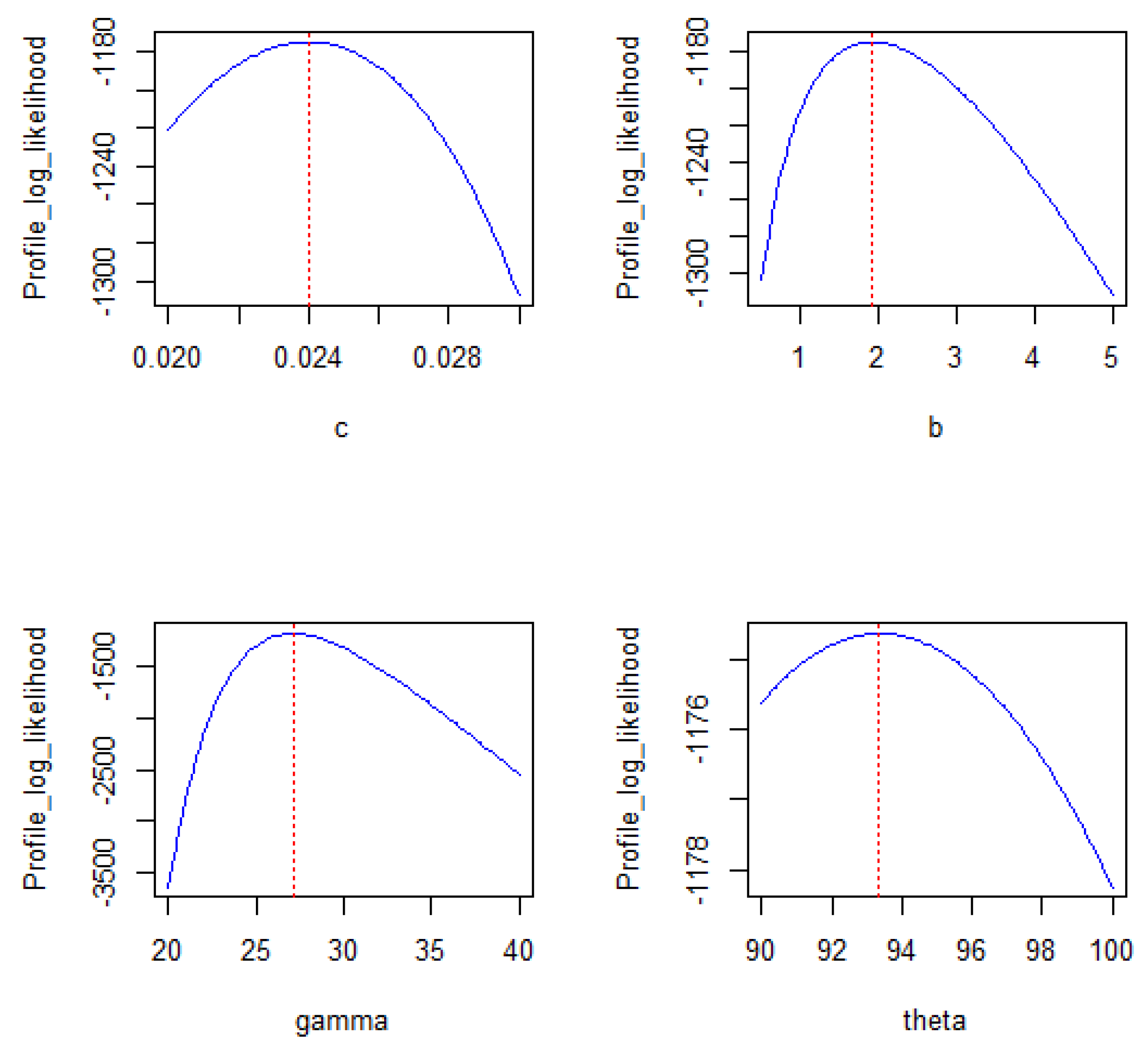
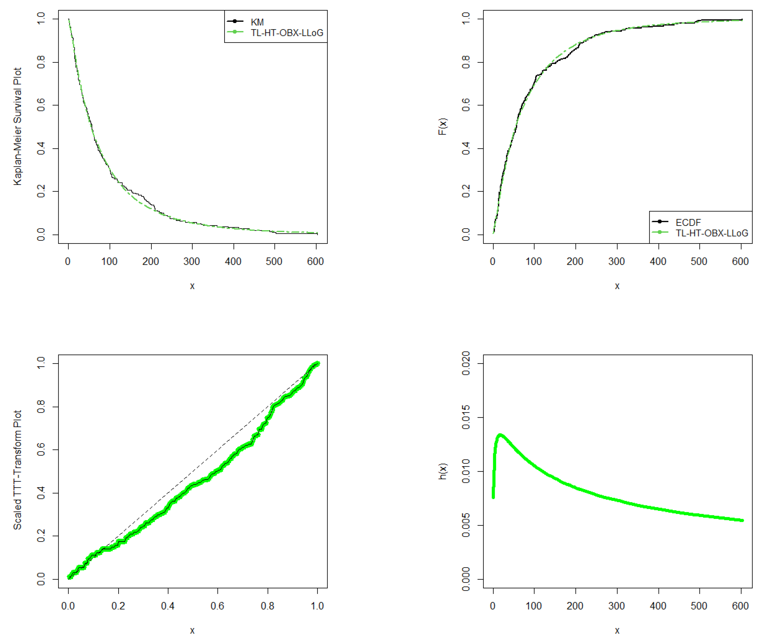
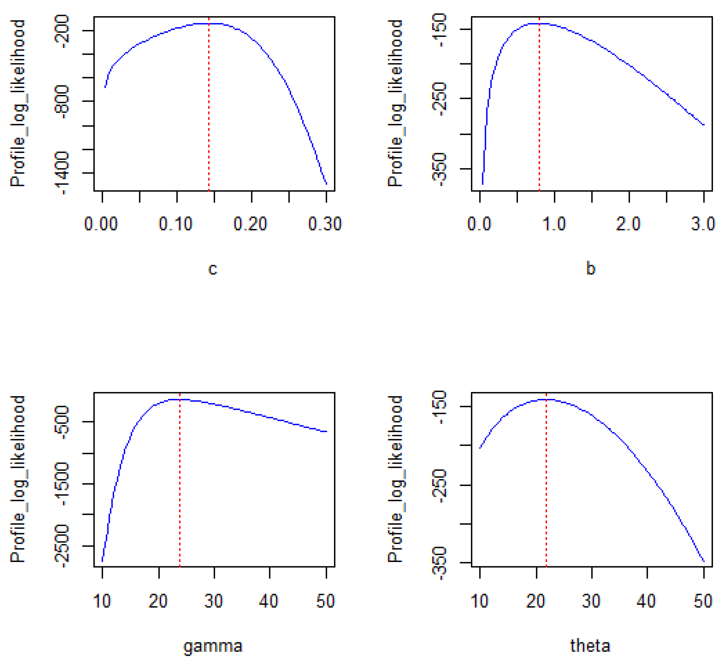
In Figure 13, we observe that the maximum likelihood estimates for the TL-HT-OBX-LLoG distribution exist and can be obtained uniquely on air conditioning system data. Figure 14 shows the fitted Kaplan–Meier (K-M) survival curve, empirical cumulative distribution function (ECDF), the scaled total time on test (TTT) transform plot, and the fitted HRF for the air conditioning system data. The fitted CDF is close to the empirical CDF, while the survival function closely follows the empirical Kaplan–Meier curve, indicating that our model is a good fit for this dataset. The scaled TTT transform plot shows an HRF with an upside-down bathtub shape, which is captured by the proposed model.

8.3. Carbon Fiber Data

The third dataset represents tensile-strength data for 100 carbon fibers, as reported by Nichols and Padgett [20] and recently analyzed by Shakil et al. [21].

The results in

Table 7. MLEs and goodness-of-fit statistics for carbon fiber data.

	Estimates				Statistics
Model	$\mathit{b}$	$\mathit{\theta }$	$\mathit{\gamma }$	$\mathit{c}$	$-\mathbf{2}log\left(\mathit{L}\right)$	$\mathit{AIC}$	$\mathit{AICC}$	$\mathit{BIC}$	${\mathit{W}}^{*}$	${\mathit{A}}^{*}$	K-S	p-Value
TL-HT-OBX-LLoG	0.7903	21.8224	23.7367	0.1432	282.6951	290.6951	291.1162	301.1158	0.0698	0.4112	0.0646	0.7978
	(0.3979)	(0.4300)	(3.8674)	(0.0288)
	b	$\delta$	$\gamma$	$\lambda$
TL-MO-W	3.3659	2.3309	1.2030	0.4678	284.4367	292.4367	292.8578	302.8574	0.1171	0.5965	0.0899	0.3933
	(3.6182)	(2.3762)	(0.9359)	(0.8570)
	$\alpha$	$\theta$	$\lambda$	$\beta$
TLGW	0.7550	0.6563	0.2294	4.3882	287.3756	295.3756	295.7966	305.7962	0.0829	0.6607	0.0808	0.5311
	(0.2470)	(0.26670)	(0.0180)	(1.1956)
	$\alpha$	$\beta$	b	$\lambda$
TL-OBIII-LLoG	110.5900	11.4590	$5.{0067}^{-01}$	$1.7512\times {10}^{-02}$	307.5220	315.5220	315.9431	325.9427	0.4058	2.2273	0.1350	0.0520
	($5.5000\times {10}^{-05}$)	(6.5830)	($3.1851\times {10}^{-01}$)	($1.5995\times {10}^{-03}$)
	$\delta$	b	$\alpha$	c
RBTL-GOM-LLoG	111.7200	981.5200	1.0785	$8.8311\times {10}^{-02}$	296.4615	304.4616	304.8826	314.8823	0.2731	1.4586	0.1175	0.1264
	($1.7026\times {10}^{-04}$ )	($2.1445\times {10}^{-05}$)	($1.7789\times {10}^{-02}$)	($6.6546\times {10}^{-03}$)
	$\alpha$	a	b	c
APExLLD	897.0300	2.3362	$7.7112\times {10}^{-02}$	321.8300	319.9412	327.9412	328.3623	338.3619	0.5611	3.1168	0.1384	0.0433
	$(1.9509\times {10}^{-06}$)	($1.4985\times {10}^{-01}$)	($1.5782\times {10}^{-02}$)	($3.8694\times {10}^{-06}$)

show that the TL-HT-OBX-LLoG distribution outperformed the non-nested models. This assertion is supported, as the TL-HT-OBX-LLoG distribution has the lowest goodness-of-fit statistics. Furthermore, among all models applied to the carbon fiber data, the TL-HT-OBX-LLoG distribution has the highest p-value for the K–S statistic. As a result, it is considered the best fit for the carbon fiber dataset. The TL-HT-OBX-LLoG distribution outperformed the non-nested models in representing the carbon fiber dataset in Figure 15.

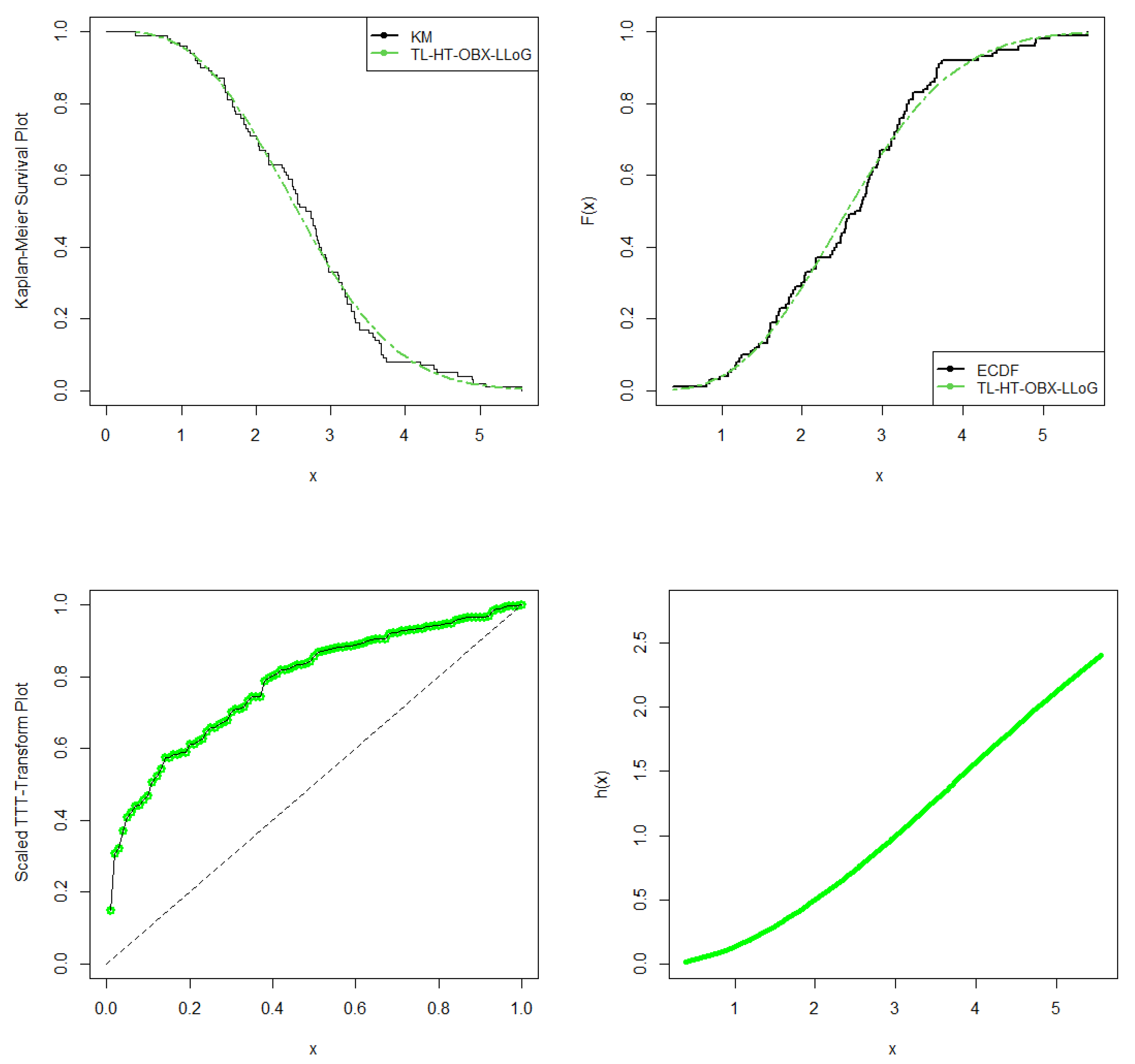
In Figure 16, we observe that the ML estimates for the TL-HT-OBX-LLoG distribution exist and can be achieved uniquely for carbon fiber data. Figure 17 shows the fitted K-M survival curve (a), ECDF (b), the TTT scaled plot (c), and the fitted hrf (d) for the carbon fiber data. The fitted CDF closely aligns with the empirical CDF, and the survival function closely resembles the empirical Kaplan-Meier curve, indicating that our model is the best fit. The scaled TTT transform plot depicts a HRF an increasing bathtub, indicating that the HRF of the carbon fibers is increasing over time which is accurately captured by the new proposed model.

9. Concluding Remarks

This paper introduces the Topp–Leone Heavy-Tailed Odd Burr X-G (TL-HT-OBX-G) FoD and examines some of its statistical properties. The new FOD is a combination of three generators, which brings a new framework of data modelling. The distribution addresses some of the limitations of heavy-tailed FOD since the new distribution applies to several forms of data, including heavy-tailed and almost symmetric data. We employed different estimation methods to obtain estimates of the model parameters and investigated three special cases of this new family of distributions. Based on the simulation results, the ML estimation approach appears highly effective for estimating the parameters of the TL-HT-OBX-LLoG distribution. We presented risk measures and numerical studies, demonstrating that the TL-HT-OBX-LLoG distribution is heavier than the selected non-nested models. Furthermore, the practical applications demonstrate that the TL-HT-OBX-LLoG distribution can be effectively used to fit heavy-tailed data and almost symmetric data, as shown in Section 8. The proposed model outperformed the selected competing models in all the instances. Therefore, the TL-HT-OBX-G offers a versatile framework for data modelling. This suggests that the TL-HT-OBX-LLoG distribution could be used in a variety of applications. In the future, we intend to expand to bivariate extensions and apply the Bayesian method for parameter estimation.

References

1. Zhao, W.; Khosa, S.K.; Ahmad, Z.; Aslam, M.; Afify, A.Z. Type-I Heavy Tailed Family with Applications in Medicine, Engineering and Insurance. PLoS ONE 2020, 15, e0237462. [Google Scholar] [CrossRef] [PubMed]
2. Lekono, G.J.; Oluyede, B.; Gabaitiri, L. A New Heavy-Tailed Exponentiated Generalised-G Family of Distributions: Properties and Applications. Int. J. Math. Oper. Res. 2024, 27, 1–34. [Google Scholar] [CrossRef]
3. Moakofi, T.; Oluyede, B. The Type I Heavy-Tailed Odd Power Generalized Weibull-G Family of Distributions with Applications. Commun. Fac. Sci. Univ. Ank. Ser. A1 Math. Stat. 2023, 72, 921–958. [Google Scholar] [CrossRef]
4. Zhao, J.; Ahmad, Z.; Mahmoudi, E.; Hafez, E.H.; Mohie El-Din, M.M. A New Class of Heavy-Tailed Distributions: Modeling and Simulating Actuarial Measures. Complexity 2021, 2021, 1–18. [Google Scholar] [CrossRef]
5. Teamah, A.E.A.; Elbanna, A.A.; Gemeay, A.M. Heavy-Tailed Log-Logistic Distribution: Properties, Risk Measures and Applications. Stat. Optim. Inf. Comput. 2021, 9, 910–941. [Google Scholar] [CrossRef]
6. Afify, A.Z.; Gemeay, A.M.; Ibrahim, N.A. The Heavy-Tailed Exponential Distribution: Risk Measures, Estimation, and Application to Actuarial Data. Mathematics 2020, 8, 1276. [Google Scholar] [CrossRef]
7. Ahmad, Z.; Mahmoudi, E.; Alizadeh, M.; Roozegar, R.; Afify, A.Z. The Exponential T-X Family of Distributions: Properties and an Application to Insurance Data. J. Math. 2021, 2021, 5580228. [Google Scholar] [CrossRef]
8. Ahmad, Z.; Mahmoudi, E.; Hamedani, G.; Kharazmi, O. New Methods to Define Heavy-Tailed Distributions with Applications to Insurance Data. J. Taibah Univ. Sci. 2020, 14, 359–382. [Google Scholar] [CrossRef]
9. Al-Shomrani, A.; Arif, O.; Shawky, A.; Hanif, S.; Shahbaz, M.Q. Toppe-Leone Family of Distributions: Some Properties and Application. Pak. J. Stat. Oper. Res. 2016, 12, 443–451. [Google Scholar] [CrossRef]
10. Haitham, M.Y.; Afify, A.Z.; Hamedani, G.G.; Aryal, G. The Burr X Generator of Distributions for Lifetime Data. J. Stat. Theory Appl. 2017, 16, 288–305. [Google Scholar] [CrossRef]
11. Shaked, M.; Shanthikumar, J.G. Stochastic Orders and their Applications; Associated Press: New York, NY, USA, 1994. [Google Scholar]
12. Rényi, A. On Measures of Entropy and Information. In Proceedings of the Fourth Berkeley Symposium on Mathematical Statistics and Probability, Berkeley, CA, USA, 20 June–30 July 1961; Volume 4, pp. 547–562. [Google Scholar]
13. Moakofi, T.; Oluyede, B.; Gabanakgosi, M. The Topp–Leone odd Burr III-G Family of Distributions: Model, Properties and Applications. Stat. Optim. Inf. Comput. 2022, 10, 236–262. [Google Scholar] [CrossRef]
14. Chen, G.; Balakrishnan, N. A General Purpose Approximate Goodness-of-Fit Test. J. Qual. Technol. 1995, 27, 154–161. [Google Scholar] [CrossRef]
15. Chambers, J.M.; Cleveland, W.S.; Kleiner, B.; Tukey, P.A. Graphical Methods for Data Analysis; Chapman and Hall/CRC: Boca Raton, FL, USA, 1983. [Google Scholar]
16. Chipepa, F.; Oluyede, B.; Makubate, B. The Topp–Leone-Marshall-Olkin-G Family of Distributions with Applications. Int. J. Stat. Probab. 2020, 9, 15–32. [Google Scholar] [CrossRef]
17. Aryal, G.R.; Ortega, E.M.; Hamedani, G.G.; Yousof, H.M. The Topp–Leone Generated Weibull Distribution: Regression Model, Characterizations and Applications. Int. J. Stat. Probab. 2017, 6, 126–141. [Google Scholar] [CrossRef]
18. Pu, S.; Moakofi, T.; Oluyede, B. The Ristić–Balakrishnan–Topp–Leone–Gompertz-G Family of Distributions with Applications. J. Stat. Theory Appl. 2023, 22, 116–150. [Google Scholar] [CrossRef]
19. Muhammad, M.; Yahaya, M.A. The Half Logistic-Poisson Distribution. Asian J. Math. Appl. 2017, 2017. [Google Scholar]
20. Nichols, M.D.; Padgett, W. A Bootstrap Control Chart for Weibull Percentiles. Qual. Reliab. Eng. Int. 2006, 22, 141–151. [Google Scholar] [CrossRef]
21. Shakil, M.; Kibria, B.; Ahsanullah, M. Some Inferences on Dagum (4P) Distribution: Statistical Properties, Characterizations and Applications. World Sci. News 2021, 154, 1–33. [Google Scholar]
Figure 1. PDF and HRF plots for TL-HT-OBX-LLoG distribution for selected parameter values.
Symmetry 17 02093 g001
Figure 2. SK and KT plots for TL-HT-OBX-LLoG distribution for selected parameter values.
Symmetry 17 02093 g002
Figure 3. PDF and HRF plots for TL-HT-OBX-W distribution for selected parameter values.
Symmetry 17 02093 g003
Figure 4. SK and KT plots for TL-HT-OBX-W distribution for selected parameter values.
Symmetry 17 02093 g004
Figure 5. Plots of the PDF and HRF for TL-HT-OBX-Lx distribution for selected parameter values.
Symmetry 17 02093 g005
Figure 6. SK and KT plots for TL-HT-OBX-Lx distribution for selected parameter values.
Symmetry 17 02093 g006
Figure 7. Plots of RMSEs from Table 1.
Symmetry 17 02093 g007
Figure 8. Plots of RMSEs from Table 2.
Symmetry 17 02093 g008
Figure 9. Fitted density superimposed on the histogram and observed probability vs expected probability plots for European COVID-19 data.
Symmetry 17 02093 g009
Figure 10. Profile log-likelihood function plots for the European COVID-19 dataset.
Symmetry 17 02093 g010
Figure 11. Fitted K–M, ECDF, TTT, and HRF plots for the European COVID-19 dataset.
Symmetry 17 02093 g011
Figure 12. Fitted density superimposed on the histogram and observed probability vs expected probability plots for air conditioning system data.
Symmetry 17 02093 g012
Figure 13. Plots of the profile log-likelihood function of the parameters of the TL-HT-OBX-LLoG distribution on air conditioning system data.
Symmetry 17 02093 g013
Figure 14. Fitted K-M, ECDF, the TTT, and HRF for air conditioning system data.
Symmetry 17 02093 g014
Figure 15. Fitted density superimposed on the histogram and observed probability vs. expected probability plots for carbon fibers data.
Symmetry 17 02093 g015
Figure 16. Plots of the profile log-likelihood function of the parameters of the TL-HT-OBX-LLoG distribution on carbon fiber data.
Symmetry 17 02093 g016
Figure 17. Fitted K-M, ECDF, TTT, and HRF plots for carbon fiber data.
Symmetry 17 02093 g017