Integrated Adaptive Robust Control for Pipe Robots Facing Compound Uncertainties

Abstract

To address the challenges of low control accuracy and poor robustness for pipe robots operating in complex environments with compound uncertainties, including parameter variations, nonlinear friction, and external disturbances, this paper proposes an integrated adaptive robust control strategy. The framework begins by establishing a high-fidelity dynamic model that considers arbitrary pipe inclination. Subsequently, a Finite-Time Disturbance Observer (FTDO) is designed to rapidly and accurately estimate and compensate for the lumped uncertainties, thereby enhancing the system’s disturbance rejection capabilities. Based on this compensation, an Adaptive Non-singular Terminal Sliding Mode Control (ANTSMC) law is synthesized. By adjusting its gain online, the controller handles unknown uncertainty bounds, ensures the finite-time convergence of tracking errors, and effectively suppresses chattering. Simulation results validate that the proposed method achieves high-precision trajectory tracking with smooth control inputs and strong robustness, even in the presence of significant uncertainties. This study offers an effective solution for the high-precision and robust motion control of pipe robots.

1. Introduction

Pipelines, serving as the “arteries” of modern industry and urban infrastructure, play an indispensable role in sectors such as oil and gas, chemical engineering, and water supply [1,2]. However, during their long-term service in complex and often harsh environments, pipeline systems are inevitably susceptible to various defects, including corrosion, cracks, and blockages, which severely threaten their structural integrity and operational safety [3]. Consequently, the development of efficient and reliable in-pipe robots designed for specific maintenance tasks, such as automated rust removal, to replace high-risk, low-efficiency manual operations has emerged as a critical research direction [4]. This endeavor is paramount for ensuring the safety of critical infrastructure and reducing operation and maintenance (O\&M) costs, thereby holding significant societal and economic value.

Despite considerable advancements in the field of pipe robotics, achieving high-precision and high-robustness autonomous control for tasks like rust removal remains a formidable challenge. The dynamic behavior of the robot is an inherently high-dimensional, strongly coupled, and nonlinear process [5]. Compounding this complexity, the robot is inevitably subjected to various uncertainties during practical operation, which can be primarily categorized as: (1) Parametric uncertainties: The precise values of the robot’s physical parameters, such as mass and moment of inertia, are difficult to obtain due to manufacturing tolerances, payload variations, or component wear [6]. (2) Unmodeled dynamics: Complex nonlinear forces, such as the friction between the wheels and the pipe wall, which exhibit characteristics like the Stribeck effect and hysteresis, are difficult to describe accurately with simple models [7,8]. (3) External disturbances: These include unknown forces and torques arising from fluid impacts within the pipe, cable drag, and interactions with obstacles [9]. These uncertainties severely degrade the performance of conventional control algorithms, leading to a deterioration in tracking accuracy and even system instability.

To address the aforementioned challenges, extensive research has been conducted by scholars worldwide. Proportional-Integral-Derivative (PID) control is widely adopted due to its simple structure and ease of implementation [10]. However, as an essentially linear controller, its performance is limited when dealing with strongly nonlinear and time-varying systems, making it difficult to meet high-precision tracking requirements. To this end, advanced nonlinear control strategies have been introduced into the field of robotics. Sliding Mode Control (SMC) has garnered significant attention for its strong robustness against matched uncertainties and external disturbances [11,12]. Nevertheless, standard SMC suffers from two inherent drawbacks: first, its discontinuous switching term tends to induce the “chattering” phenomenon, which can excite high-frequency unmodeled dynamics and damage actuators [13]; second, it only guarantees asymptotic convergence of the tracking error, failing to achieve stability within a finite time. To achieve finite-time convergence, Terminal Sliding Mode Control (TSMC) was proposed [14]. However, its control law contains negative fractional power terms, leading to a singularity problem when the error approaches zero [15]. Non-singular Terminal Sliding Mode Control (NTSMC), by modifying the sliding surface design, successfully resolves the singularity issue, emerging as a more practical option [16,17].

On the other hand, the Disturbance Observer (DO), based on the “estimate and compensate” paradigm, offers another effective approach for handling lumped uncertainties [18,19]. By online estimating the total disturbance acting on the system and compensating for it in a feedforward manner, a DO can significantly enhance the system’s disturbance rejection capability. However, conventional linear DOs face an inherent trade-off between estimation speed and noise sensitivity: a high gain can accelerate estimation but also amplifies measurement noise. To address this issue, nonlinear DOs, particularly the Finite-Time Disturbance Observer (FTDO), have gained increasing attention for their ability to accurately estimate disturbances within a finite time [20,21,22]. Furthermore, for parametric uncertainties, adaptive control, through online tuning of controller parameters, can effectively track slowly time-varying parameters, but its robustness against unmodeled dynamics and external disturbances is relatively weak [23,24].

In summary, no single control strategy can comprehensively address the composite uncertainties faced by pipe robots in complex environments. Therefore, developing a hybrid control framework that integrates the merits of multiple advanced strategies is an inevitable trend for enhancing robot control performance. While previous studies have explored methods such as adaptive sliding mode [23,25] and the combination of DO with SMC [16,26], the design of an integrated control framework for pipe robot systems---one that can rapidly compensate for unknown disturbances, adapt to parametric uncertainties, and simultaneously guarantee finite-time convergence of tracking errors---remains an open and challenging research problem [27].

In light of the foregoing, this paper proposes an integrated adaptive robust control framework for a class of coupled 2-degree-of-freedom (2-DOF) pipe robot systems, comprising an axial crawler and a single-link manipulator. This framework is tailored to address the high-precision trajectory tracking control problem in complex and realistic pipeline environments. The main contributions and innovations of this paper are as follows. First, a high-fidelity dynamic model is established, which considers arbitrary pipe inclination angles and nonlinear friction. This model significantly enhances the controller’s adaptability and precision in complex, real-world pipeline environments, laying a solid physical foundation for subsequent environment-aware control design. Second, a novel control scheme based on a Finite-Time Disturbance Observer (FTDO) is proposed to actively estimate and compensate for lumped uncertainties. This method improves tracking accuracy and suppresses chattering by minimizing the reliance on high-gain feedback. Finally, an Adaptive Non-singular Terminal Sliding Mode Controller (ANTSMC) is designed to guarantee finite-time convergence without requiring prior knowledge of the uncertainty bounds. This design optimizes control energy consumption and enhances the system’s robustness to residual estimation errors.

The remainder of this paper is organized as follows. Section 2 establishes the high-fidelity dynamic model of the pipe inspection robot by applying the Euler-Lagrange formalism, with special attention to environmental factors such as pipe inclination and nonlinear friction. Section 3 details the design of the hierarchical robust adaptive control architecture, which includes the state observer, the nonlinear disturbance observer, and the core adaptive NTSMC law, followed by a rigorous stability analysis of the composite system. Section 4 addresses key practical refinements for implementation, including chattering suppression and strategies for handling actuator saturation. In Section 5, comprehensive simulation studies are presented to validate the effectiveness and demonstrate the superior performance of the proposed control strategy. Finally, Section 6 concludes the paper with a summary of the key findings and contributions.

2. High-Fidelity Dynamic Modeling for Complex Environments

The development of a high-performance robust adaptive control framework for a 1-DOF pipe inspection robot necessitates, as a primary task, the establishment of a dynamic model that accurately reflects its physical behavior in complex, real-world environments. Pipe inspection robots operate under uniquely challenging conditions, including navigating long distances within confined and often unstructured pipelines, encountering unpredictable surface conditions, and operating at various angles of inclination. Conventional models frequently oversimplify the system by neglecting crucial environmental factors such as the gravitational effects of varying pipe inclinations and the complex, nonlinear nature of friction. Such simplifications can lead to a significant model-plant mismatch, resulting in degraded controller performance, poor tracking accuracy, and even instability in practical applications.

Therefore, this section is dedicated to the systematic derivation of a high-fidelity dynamic model using first principles. This model aims to encapsulate the dominant dynamic effects encountered during operation. It not only provides a solid physical foundation for the subsequent controller design but also serves as the essential prerequisite for developing a truly environment-aware and robust control system capable of high-precision motion tasks.

2.1. System Kinematics and Energy in Inclined Pipes

We begin by defining the system’s configuration via the generalized coordinate vector $q={[x,\theta ]}^T$, as depicted in Figure 1. Here, $x$ represents the axial displacement of the robot’s main body along the pipe’s central axis, and $\theta$ is the angular position of the single-link manipulator relative to the robot’s body. To generalize the model for any operational scenario, we consider the pipe to be at an arbitrary inclination angle $\varphi$ with respect to the horizontal.

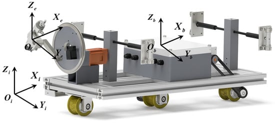
Figure 1. Schematic diagram of the pipeline rust removal robot, illustrating the generalized coordinates $x$ (axial displacement) and $\theta$ (manipulator angle) within an inclined pipe.

The kinetic energy of the system, $T$, is the sum of the translational energy of the main body and the combined translational and rotational energy of the manipulator. To formulate this, let us define the system’s parameters and state variables. The mass of the robot’s main body is denoted by $m_b$, and its linear position along the pipe’s axis is given by $x$. Consequently, its linear velocity is $\dot{x}$. The manipulator arm is characterized by its mass $m_a$, its moment of inertia about the pivot point $I_a$, and the distance from the pivot to its center of mass $l_a$. The angle of the manipulator arm relative to a reference axis (e.g., perpendicular to the pipe) is $\theta$, with an angular velocity of $\dot{\theta }$.

The total kinetic energy is composed of three parts: (1) the translational kinetic energy of the main body, (2) the translational kinetic energy of the manipulator’s center of mass, which is affected by both the body’s velocity $\dot{x}$ and the arm’s rotation $\dot{\theta }$, and (3) the rotational kinetic energy of the manipulator arm about its center of mass. Following a standard kinematic analysis, the total kinetic energy is formulated as:

$$T={\displaystyle \frac{1}{2}}{m}_b{\dot{x}}^2+{\displaystyle \frac{1}{2}}{m}_a({\dot{x}}^2-2\dot{x}\dot{\theta }{l}_a\sin \theta +l_a^2{\dot{\theta }}^2)+{\displaystyle \frac{1}{2}}{I}_a{\dot{\theta }}^2.$$

(1)

Although the structure of the expression of the kinetic energy is independent of the inclination of the pipe, the potential energy, $V$, is fundamentally altered by the influence of gravity. The potential energy of the system depends on the acceleration due to gravity $g$ and the pipe’s inclination angle $\varphi$ with respect to the horizontal. It is given by:

$$V=(m_b+m_a)gx\sin \varphi +m_{a}g{l}_a\cos \varphi \sin \theta .$$

(2)

This expression reveals two critical gravitational effects. The first term, $(m_b+m_a)gx\sin \varphi$, introduces a significant potential energy gradient along the axial direction, creating a constant gravitational force that the propulsion system must overcome when moving uphill or that assists motion when moving downhill. The second term, $m_{a}g{l}_a\cos \varphi \sin \theta$, shows that the gravitational torque acting on the manipulator is modulated by the pipe’s inclination via the $\cos \varphi$ factor. This is a critical consideration for precise tool orientation, as the torque required to hold the arm at a given angle $\theta$ changes with the robot’s position in the pipeline network.

2.2. Derivation of the Full Dynamic Equation

Applying the Euler-Lagrange formalism, where the Lagrangian is defined as $\mathcal{L}=T-V$, the equations of motion are derived from ${\displaystyle \frac{d}{dt}}\left({\displaystyle \frac{\partial \mathcal{L}}{\partial \dot{q}}}\right)-{\displaystyle \frac{\partial \mathcal{L}}{\partial q}}=Q_{nc}$, where $Q_{nc}$ represents the non-conservative forces and torques, including control inputs $\tau$ and friction forces $F_f$. This procedure yields the complete dynamic equation of the system in a standard matrix form:

$$M(q)\ddot{q}+C(q,\dot{q})\dot{q}+G(q,\varphi )+F_f(\dot{q})=\tau ,$$

(3)

where the inertia matrix $M(q)$ is symmetric and positive-definite, and the Coriolis/centrifugal matrix $C(q,\dot{q})$ captures the velocity-dependent coupling terms. The gravity vector $G(q,\varphi )$ and a sophisticated friction vector $F_f(\dot{q})$ are defined as:

$$G(q,\varphi )={\displaystyle \frac{\partial V}{\partial q}}=\left[\begin{array}{c}(m_b+m_a)g\sin \varphi \\ m_{a}g{l}_a\cos \varphi \cos \theta \end{array}\right], F_f(\dot{q})=\left[\begin{array}{c}{F}_{c,x}\mathrm{sgn}(\dot{x})+F_{v,x}\dot{x}\\ F_{c,\theta }\mathrm{sgn}(\dot{\theta })+F_{v,\theta }\dot{\theta }\end{array}\right]$$

(4)

The friction vector $F_f(\dot{q})$ represents a significant modeling enhancement beyond simple linear models. In this formulation, we explicitly include both Coulomb ($F_c$) and viscous ($F_v$) friction components, which capture the dominant dissipative effects at low and high velocities, respectively. More advanced representations, such as LuGre-type models, could further encapsulate complex nonlinear phenomena like pre-sliding displacement and frictional lag. These effects, while not explicitly used in the controller design to maintain simplicity, are included in the high-fidelity simulation plant to represent unmodeled dynamics. The resulting model (3) provides a rich, physically meaningful representation of the robot’s interaction with its environment, posing a formidable challenge for control design due to its strong nonlinearities and couplings.

3. Hierarchical Robust Adaptive Control Architecture

Building upon the high-fidelity dynamic model, we engineer a hierarchical control architecture designed for ultimate performance and robustness against the identified complexities. A simple linear controller, such as a PID, would struggle to provide uniform performance across the entire operating range due to the state-dependent nature of the system’s dynamics and the presence of significant, unpredictable disturbances. Our proposed strategy is therefore multi-layered, adopting a “divide and conquer” philosophy to systematically address each challenge. First, a state observer reconstructs velocity information from position data, avoiding noise amplification from direct differentiation. Second, a disturbance observer estimates and actively compensates for the lumped uncertainties. Finally, an adaptive non-singular terminal sliding mode control (NTSMC) layer provides a robust feedback mechanism to guarantee finite-time error convergence and system stability. The control flow diagram for the entire system is shown in Figure 2. Content has been added to the original text.

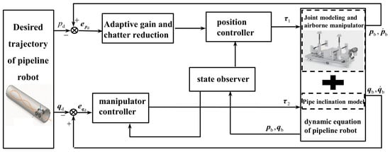
Figure 2. Flowchart of the proposed integrated control structure, illustrating the signal flow from desired trajectory to final control torque, including state observation, disturbance estimation, and the adaptive NTSMC core.

3.1. Problem Formulation with Lumped Disturbance

To structure the control problem, we partition the full system dynamics (3) into a known nominal part (subscript $n$) and an unknown lumped disturbance vector, $d(t)$. The nominal model, $M_n(q)$, $C_n(q,\dot{q})$, and $G_n(q,\varphi )$, is what the controller uses for its calculations and contains parameter estimates that may be inaccurate. The dynamics can then be rewritten as:

$$M_n(q)\ddot{q}+C_n(q,\dot{q})\dot{q}+G_n(q,\varphi )=\tau -d(t).$$

(5)

This lumped disturbance $d(t)$ is a comprehensive representation of all modeling imperfections and external wrenches, defined as:

$$\begin{array}{ll}d(t)=\hfill & \underset{\mathrm{Parametric} \mathrm{Uncertainties}}{\underbrace{(\Delta M(q)\ddot{q}+\Delta C(q,\dot{q})\dot{q}+\Delta G(q,\varphi ))}} \hfill \\ \hfill & +\underset{\mathrm{Unmodeled} \mathrm{Dynamics}}{\underbrace{F_f(\dot{q})}}+\underset{\mathrm{External} \mathrm{Disturbances}}{\underbrace{{\tau }_{ext}(t)}}\hfill \end{array}$$

(6)

where $\Delta M=M-M_n$, $\Delta C=C-C_n$, and $\Delta G=G-G_n$ represent the structural uncertainties arising from inaccurate parameter estimates. The primary control challenge is to design a control law $\tau$ that ensures high-performance tracking of a desired trajectory $q_d(t)$ by effectively rejecting $d(t)$ without its direct measurement.

3.2. State and Velocity Estimation from Position Data

A major practical limitation in most robotic systems is that joint velocities ($\dot{q}$) and accelerations ($\ddot{q}$) are not measured directly. While positions ($q$) are accurately available from encoders, obtaining velocities via numerical differentiation of these signals is notoriously problematic, as it significantly amplifies measurement noise and can degrade controller performance. To circumvent this, we design a state observer to provide clean and reliable estimates. A high-gain observer is a suitable and well-established choice for this task:

$$\begin{array}{l}\dot{\widehat{q}}=\widehat{\dot{q}}+H_1(q-\widehat{q})\\ \dot{\widehat{\dot{q}}}=M_n^{-1}(\tau -C_n\widehat{\dot{q}}-G_n)+H_2(q-\widehat{q})\end{array}$$

(7)

where $\widehat{q}$ and $\widehat{\dot{q}}$ are the estimated position and velocity, respectively. $H_1$ and $H_2$ are diagonal positive-definite observer gain matrices, typically chosen as $H_1=h_{1}I$ and $H_2=h_{2}I$. The large positive constants $h_1,h_2$ create fast error dynamics, ensuring that the estimation errors $(\tilde{q},\tilde{\dot{q}})=(q-\widehat{q},\dot{q}-\widehat{\dot{q}})$ converge to zero rapidly. Henceforth, the controller will exclusively utilize the estimated states $(\widehat{q},\widehat{\dot{q}})$ for all feedback calculations.

To actively compensate for the lumped disturbance, we employ a nonlinear disturbance observer (NDO). Unlike a simple filter, an NDO uses the system’s nominal model to achieve a more accurate and faster estimation. To do this, we define an auxiliary variable $p$ which represents the “calculable” parts of the dynamics using the nominal model (with subscript $n$) and the estimated states (from Section 3.2), $\widehat{\dot{q}}$ and $\ddot{\widehat{q}}$:

$$p=M_n\ddot{\widehat{q}}+C_n\widehat{\dot{q}}+G_n-\tau$$

(8)

The disturbance estimate, $\widehat{d}$, is then constructed using the following nonlinear observer law, where $L$ is a positive-definite gain matrix:

$$\dot{\widehat{d}}=-L(\widehat{d}+p)$$

(9)

The estimated disturbance $\widehat{d}$ is then fed forward to the main controller to cancel the real disturbance in real-time.

To formally analyze the convergence of the NDO, we examine the estimation error dynamics for $\tilde{d}=d-\widehat{d}$. Taking its time derivative, $\dot{\tilde{d}}=\dot{d}-\dot{\widehat{d}}$. Substituting our observer law (10):

$$\dot{\tilde{d}}=\dot{d}+L(\widehat{d}+p)$$

(10)

We now substitute $\widehat{d}=d-\tilde{d}$ and the definition of $p$:

$$\dot{\tilde{d}}=\dot{d}+L((d-\tilde{d})+(M_n\ddot{\widehat{q}}+C_n\widehat{\dot{q}}+G_n-\tau ))$$

(11)

We use the estimation errors from Section 3.2: ${\widehat{e}}_2=\dot{q}-\widehat{\dot{q}}$ and its derivative ${\dot{\widehat{e}}}_2=\ddot{q}-\ddot{\widehat{q}}$. Substituting $\widehat{\dot{q}}=\dot{q}-{\widehat{e}}_2$ and $\ddot{\widehat{q}}=\ddot{q}-{\dot{\widehat{e}}}_2$:

$$\dot{\tilde{d}}=\dot{d}+L((d-\tilde{d})+(M_n(\ddot{q}-{\dot{\widehat{e}}}_2)+C_n(\dot{q}-{\widehat{e}}_2)+G_n-\tau ))$$

(12)

By regrouping terms based on the true system dynamics defined in Equation (7) (i.e.,$M_n\ddot{q}+C_n\dot{q}+G_n-\tau =-d$), the expression simplifies:

$$\begin{array}{l}\dot{\tilde{d}}=\dot{d}+L((d-\tilde{d})+(M_n\ddot{q}+C_n\dot{q}+G_n-\tau )-M_n{\dot{\widehat{e}}}_2-C_n{\widehat{e}}_2)\\ \dot{\tilde{d}}=\dot{d}+L((d-\tilde{d})+(-d)-M_n{\dot{\widehat{e}}}_2-C_n{\widehat{e}}_2)\\ \dot{\tilde{d}}+L\tilde{d}=\dot{d}-L(M_n{\dot{\widehat{e}}}_2+C_n{\widehat{e}}_2)\end{array}$$

(13)

This final equation represents the NDO error dynamics. To formally analyze its stability, we rearrange it as:

$$\dot{\tilde{d}}=-L\tilde{d}+\delta (t)$$

(14)

where $\delta (t)=\dot{d}-L(M_n{\dot{\widehat{e}}}_2+C_n{\widehat{e}}_2)$ is a perturbation term.

We can now prove the stability of the NDO using a Lyapunov analysis. As established in Section 3.2, the high-gain state observer guarantees that the state estimation errors ${\widehat{e}}_2$ and ${\dot{\widehat{e}}}_2$ are bounded. Furthermore, we assume the lumped disturbance $d$ is slowly varying (a standard assumption for physical uncertainties), meaning its derivative $\dot{d}$ is also bounded. Consequently, the entire perturbation term $\delta (t)$ is bounded by some positive constant ${\delta }_{max}$, such that $\left|\right|\delta (t)\left|\right|\le {\delta }_{max}$.

Consider the Lyapunov function candidate:

$$V_{ndo}={\displaystyle \frac{1}{2}}{\tilde{d}}^T\tilde{d}$$

(15)

Taking the time derivative of $V_{ndo}$ along the error dynamics yields:

$$\begin{array}{l}{\dot{V}}_{ndo}={\tilde{d}}^T\dot{\tilde{d}}={\tilde{d}}^T(-L\tilde{d}+\delta (t))\\ {\dot{V}}_{ndo}=-{\tilde{d}}^{T}L\tilde{d}+{\tilde{d}}^T\delta (t)\end{array}$$

(16)

Using standard vector norm inequalities and the definition of ${\delta }_{max}$:

$$\begin{array}{l}{\dot{V}}_{ndo}\le -{\lambda }_{min}(L)\left|\right|\tilde{d}|{|}^2+|\left|\tilde{d}\right||\cdot ||\delta (t)||\\ {\dot{V}}_{ndo}\le -{\lambda }_{min}(L)\left|\right|\tilde{d}|{|}^2+|\left|\tilde{d}\right||\cdot {\delta }_{max}\\ {\dot{V}}_{ndo}\le -\left|\right|\tilde{d}\left|\right|({\lambda }_{min}(L)|\left|\tilde{d}\right||-{\delta }_{max})\end{array}$$

(17)

This derivative ${\dot{V}}_{ndo}$ is guaranteed to be negative (i.e.,${\dot{V}}_{ndo}<0$) as long as $\left|\right|\tilde{d}\left|\right|>{\displaystyle \frac{{\delta }_{max}}{{\lambda }_{min}(L)}}$. This analysis formally proves that the disturbance estimation error $\tilde{d}$ is Uniformly Ultimately Bounded (UUB). The ultimate bound $ϵ={\displaystyle \frac{{\delta }_{max}}{{\lambda }_{min}(L)}}$ can be made arbitrarily small by increasing the NDO gain $L$ (which increases ${\lambda }_{min}(L)$). This provides a rigorous justification for the observer’s stability, replacing the previous approximation, and confirms that $\tilde{d}$ converges to a small neighborhood of zero.

3.3. Integrated Robust Adaptive Control Architecture

With reliable estimates of the state and disturbances, we can synthesize the final control law. We choose a non-singular terminal sliding mode control (NTSMC) strategy to guarantee finite-time convergence of tracking errors, which is superior to the asymptotic convergence of conventional sliding mode control. The non-singular terminal sliding surface is defined using the estimated state error $\widehat{e}=\widehat{q}-q_d$:

$$s=\dot{\widehat{e}}+\alpha \widehat{e}+\beta \mathrm{sig}{(\widehat{e})}^{\gamma }$$

(18)

where $\alpha ,\beta$ are diagonal positive-definite gain matrices and $1<\gamma <2$. The term $\alpha \widehat{e}$ ensures fast convergence when the error is large, while the nonlinear term $\beta \mathrm{sig}{(\widehat{e})}^{\gamma }$ dominates when the error is small, enforcing finite-time convergence to the sliding surface.

Remark 1: The composite structure of the NTSMC surface (18) is designed to ensure both fast convergence and finite-time stability. The mathematical basis lies in the error dynamics enforced when $s=0$, i.e., ${\dot{\widehat{e}}}_1=-\alpha {\widehat{e}}_1-\beta \mathrm{sig}{({\widehat{e}}_1)}^{\gamma }$. When the error ${\widehat{e}}_1$ is large, the linear term $\alpha {\widehat{e}}_1$ dominates, resulting in fast, exponential convergence (${\dot{\widehat{e}}}_1\approx -\alpha {\widehat{e}}_1$). Conversely, when ${\widehat{e}}_1$ is small, the nonlinear term $\beta \mathrm{sig}{({\widehat{e}}_1)}^{\gamma }$ (with $0<\gamma <1$) dominates, enforcing finite-time convergence (${\dot{\widehat{e}}}_1\approx -\beta \mathrm{sig}{({\widehat{e}}_1)}^{\gamma }$). This structure thus combines the fast transient response of conventional SMC with the finite-time convergence of TSMC.

The complete, hierarchical control law is structured to combine model-based feedforward compensation with robust adaptive feedback. It is formulated as:

$$\tau ={\tau }_{eq}+{\tau }_{rob}=(C_n\dot{\widehat{q}}+G_n+M_n{\ddot{q}}_{eq})+(\widehat{d}-K_{s}s-{\widehat{K}}_{ϵ}\mathrm{sgn}(s)).$$

(19)

where ${\ddot{q}}_{eq}={\ddot{q}}_d-\alpha \dot{\widehat{e}}-\beta \gamma \mathrm{diag}({\left|{\widehat{e}}_i\right|}^{\gamma -1})\dot{\widehat{e}}$ is the equivalent acceleration required to maintain the system on the sliding surface. The control law consists of several distinct components:

• Model Compensation $(C_n\dot{\widehat{q}}+G_n+M_n{\ddot{q}}_{eq})$: This is the equivalent control part that linearizes and decouples the nominal dynamics.
• Disturbance Rejection $(\widehat{d})$: This term provides feedforward cancellation of the estimated disturbance.
• Robust Feedback $(-K_{s}s-{\widehat{K}}_{ϵ}\mathrm{sgn}(s))$: This term, composed of a proportional reaching law ($-K_{s}s$) and an adaptive discontinuous term, ensures robustness against residual disturbance estimation errors and guarantees the sliding condition is met.

The adaptive gain ${\widehat{K}}_{ϵ}$ is updated in real-time to handle the unknown bound of the residual estimation error $\tilde{d}=d-\widehat{d}$, using the simple and effective law:

$${\dot{\widehat{K}}}_{ϵ,i}={\eta }_i\left|s_i\right|,\hspace{1em}\mathrm{where} {\eta }_i>0 \mathrm{is} \mathrm{the} \mathrm{adaptive} \mathrm{rate}.$$

(20)

This ensures that the control gain is only increased when necessary (i.e., when $\left|s_i\right|>0$), preventing gain overestimation.

3.4. Stability Analysis of the Composite System

The stability of the overall system depends on the interplay between the state observer, the disturbance observer, and the controller. A formal combined proof is complex; however, under the standard and practical assumption of time-scale separation, stability can be established. By selecting the observer gains ($H_1,H_2,L$) to be sufficiently large, the estimation dynamics for both the state and the disturbance can be made significantly faster than the controller dynamics. This ensures that $\widehat{q}\to q$, $\widehat{\dot{q}}\to \dot{q}$, and $\widehat{d}\to d$ rapidly.

Under this assumption, we analyze the stability of the dominant closed-loop controller dynamics. Consider the Lyapunov function candidate for the controller subsystem:

$$V={\displaystyle \frac{1}{2}}{s}^T{M}_{n}s+{\displaystyle \frac{1}{2}}{\displaystyle \sum _{i=1}^2\frac{1}{{\eta }_i}}{({\tilde{K}}_{ϵ,i})}^2$$

(21)

where ${\tilde{K}}_{ϵ}=K_{ϵ}-{\widehat{K}}_{ϵ}$ is the adaptive gain estimation error, and $K_{ϵ}$ is an unknown ideal gain that bounds the residual disturbance. Taking the time derivative of $V$ along the system trajectories yields:

$$\begin{array}{ll}\dot{V}\hfill & =s^T{M}_n\dot{s}+s^T({\dot{M}}_n-2C_n)s-{\displaystyle \sum \frac{1}{{\eta }_i}}{\tilde{K}}_{ϵ,i}{\dot{\widehat{K}}}_{ϵ,i} \hfill \\ \hfill & =s^T(M_n\ddot{\widehat{e}}+C_n\dot{\widehat{e}})-{\displaystyle \sum {\tilde{K}}_{ϵ,i}}\left|s_i\right| \hfill \\ \hfill & =s^T(d-\widehat{d}-K_{s}s-{\widehat{K}}_{ϵ}\mathrm{sgn}(s))-{\displaystyle \sum {\tilde{K}}_{ϵ,i}}\left|s_i\right| \hfill \\ \hfill & =s^T\tilde{d}-s^T{K}_{s}s-{\displaystyle \sum {\widehat{K}}_{ϵ,i}}\left|s_i\right|-{\displaystyle \sum {\tilde{K}}_{ϵ,i}}\left|s_i\right| \hfill \\ \hfill & \le {\displaystyle \sum }\left|s_i\right|\left|{\tilde{d}}_i\right|-s^T{K}_{s}s-{\displaystyle \sum (K_{ϵ,i}-{\tilde{K}}_{ϵ,i})}\left|s_i\right|-{\displaystyle \sum {\tilde{K}}_{ϵ,i}}\left|s_i\right| \hfill \\ \hfill & ={\displaystyle \sum }\left|s_i\right|(\left|{\tilde{d}}_i\right|-K_{ϵ,i})-s^T{K}_{s}s.\hfill \end{array}$$

(22)

By choosing the ideal gain $K_{ϵ,i}\ge \left|{\tilde{d}}_i\right|$, we ensure that $\dot{V}\le -s^T{K}_{s}s\le 0$. Since $\dot{V}$ is negative semi-definite, this guarantees that $s$ is bounded. By Barbalat’s Lemma, it can be further shown that $s\to 0$ as $t\to \infty$. The convergence of the sliding variable $s$ to zero ensures the stability of the closed-loop system and, due to the structure of the NTSMC surface, the finite-time convergence of the tracking error $\widehat{e}$ to zero.

4. Practical Implementation and Refinements

While the core control algorithm is theoretically sound, several practical issues must be addressed to ensure successful, safe, and smooth deployment on a physical robot. This section details the essential refinements made to bridge the gap between theory and implementation.

4.1. Handling Input Saturation with Anti-Windup

All physical actuators have finite limits; the motors cannot deliver infinite force or torque. If the controller (19) commands a torque $\tau$ that exceeds the actuator’s maximum capability ${\tau }_{max}$, the actual applied torque ${\tau }_{sat}$ will be saturated. This discrepancy can lead to a phenomenon known as integrator windup. Because the controller is unaware of the saturation, the error integral term (implicitly embedded in the dynamics of $s$) continues to accumulate, leading to a large overshoot and poor performance when the error eventually changes sign.

To counteract this, an anti-windup mechanism is crucial. We introduce a simple but effective modification by feeding back the difference between the commanded and saturated control signals to the controller. While various sophisticated schemes exist, a common approach involves modifying the error dynamics. In our simulation, we implement this directly by applying a saturation function to the final control output, a fundamental step in any realistic simulation.

$${\tau }_{final}=\max (\min (\tau ,{\tau }_{max}),-{\tau }_{max})$$

(23)

This ensures the control signal sent to the plant model is always within physical limits, preventing numerical instability and providing a more realistic assessment of controller performance.

4.2. Chattering Mitigation via Boundary Layer

A well-known drawback of classical sliding mode control is the chattering phenomenon, which arises from the discontinuous $\mathrm{sgn}(s)$ function in the control law. This results in high-frequency oscillations in the control signal. Chattering is highly undesirable in practice as it can excite unmodeled high-frequency dynamics of the robot, cause excessive mechanical wear on gears and actuators, and increase energy consumption.

To eliminate this detrimental effect, the discontinuous signum function is replaced with a continuous saturation function, ‘sat()’, within a thin boundary layer of thickness ${\Phi }_i$ around the sliding surface $s_i=0$:

$$\mathrm{sat}(s_i/{\Phi }_i)=\left\{\begin{array}{ll}\mathrm{sgn}(s_i)\hfill & \mathrm{if} \left|s_i\right|>{\Phi }_i\hfill \\ s_i/{\Phi }_i\hfill & \mathrm{if} \left|s_i\right|\le {\Phi }_i\hfill \end{array}\right..$$

(24)

This modification creates a smooth transition in the control signal as the system state enters the boundary layer, effectively filtering out the high-frequency switching. The primary trade-off is that perfect asymptotic tracking is sacrificed; the tracking error is only guaranteed to converge to a small residual set whose size is proportional to the boundary layer thickness $\Phi$. However, this is an entirely acceptable compromise for achieving smooth, safe, and implementable control action.

4.3. Guidelines for Parameter Tuning and Selection

The performance of the proposed hierarchical controller is contingent upon the judicious selection of its various parameters. Tuning is a systematic process, often involving a combination of theoretical guidelines and empirical adjustments.

• NTSMC Gains ($\alpha ,\beta ,\gamma$): These gains shape the error convergence dynamics. $\alpha$ governs the convergence rate when the error is large, while $\beta$ and $\gamma$ dictate the speed of finite-time convergence near the origin. Increasing $\alpha$ and $\beta$ generally leads to faster error reduction but at the cost of higher control effort and potential for overshoot.
• Observer Gains ($H_1,H_2,L$): These gains determine the speed of the state and disturbance estimation. Higher gains lead to faster convergence of the estimates to their true values but also amplify measurement noise. The tuning process involves finding a balance where the estimation is significantly faster than the desired closed-loop bandwidth without introducing excessive noise into the control loop.
• Robust and Adaptive Gains ($K_s,\eta$): The switching gain $K_s$ determines the reaching speed towards the sliding surface. The adaptive rate $\eta$ controls how quickly the adaptive gain ${\widehat{K}}_{ϵ}$ grows to compensate for uncertainties. A larger $\eta$ allows for faster adaptation to changing disturbances but can also lead to higher-frequency oscillations in the adaptive gain itself.
• Boundary Layer Thickness ($\Phi$): This parameter represents a direct trade-off between chattering suppression and steady-state tracking accuracy. A larger $\Phi$ results in smoother control signals but permits a larger steady-state error. It should be chosen to be as small as possible while ensuring the chattering is adequately suppressed to an acceptable level for the physical hardware.

5. Simulation Studies

To validate the effectiveness and performance of the proposed adaptive robust control strategy, numerical simulations were conducted for the 2-DOF pipe-crawling robot (axial motion $x$ and manipulator motion $\theta$) developed in Section 2. The simulations were implemented in a MATLAB 2021b environment, considering significant parametric uncertainties, unmodeled dynamics (friction), and external time-varying disturbances. The robot is tasked with navigating along a pipe inclined at $30°$ while its manipulator executes a prescribed motion. The resulting path of the end-effector in the three-dimensional workspace is depicted in Figure 3, which provides a visual overview of the simulation task.

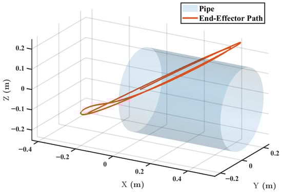
Figure 3. The 3D trajectory of the robot’s end-effector in the simulated environment.

5.1. Simulation Setup

The dynamic model of the robot is subject to uncertainties. The actual physical parameters used in the plant simulation and the nominal parameters used in the controller design are listed in Table 1. The discrepancy between the actual and nominal values constitutes the parametric uncertainty that the controller must handle.

Table 1. Robot Physical Parameters.

Parameter	Symbol	Actual Value	Nominal Value
Main body mass	$m_b$	$5.0 \mathrm{kg}$	$4.5 \mathrm{kg}$
Manipulator mass	$m_a$	$1.2 \mathrm{kg}$	$1.0 \mathrm{kg}$
Arm length (CG)	$l_a$	$0.5 \mathrm{m}$	$0.5 \mathrm{m}$
Arm inertia	$I_a$	$0.1 \mathrm{kg}\cdot {\mathrm{m}}^2$	$0.09 \mathrm{kg}\cdot {\mathrm{m}}^2$
Pipe inclination	$\varphi$	$30°$	$30°$
Gravity	$g$	$9.81 \mathrm{m}/{\mathrm{s}}^2$	$9.81 \mathrm{m}/{\mathrm{s}}^2$

The controller and observer parameters were set according to the values in Table 2. These values were chosen to ensure a stable response and demonstrate the controller’s performance.

Table 2. Controller and Observer Parameters.

Parameter	Value
State Observer Gains	$h_1=100, h_2=2500$
Disturbance Observer Gain	$L=\mathrm{diag}([2,2])$
NTSMC Gains	$\alpha =\mathrm{diag}([80,60]), \beta =\mathrm{diag}([1.5,1.5]), \gamma =1.5$
Switching Gain	$K_s=\mathrm{diag}([1,8])$
Adaptive Rate	$\eta =\mathrm{diag}([30,20])$
Boundary Layer Thickness	$\Phi =[2;2]$
Control Input Saturation	${\tau }_{\max }=[100;50] \mathrm{N},\mathrm{N}\mathrm{m}$

The desired trajectory for the robot’s joints is defined as:

$$\begin{array}{ll}{q}_{d1}(t)\hfill & =0.5\sin (0.5t)\hspace{1em}\left(\mathrm{m}\right)\hfill \\ q_{d2}(t)\hfill & =(\pi /6)\sin (0.8t)\hspace{1em}\left(\mathrm{rad}\right)\hfill \end{array}$$

(25)

The system is subjected to both unmodeled friction forces and external disturbances. The friction model includes Coulomb and viscous components: $F_f=[F_{c,x}\mathrm{sgn}({\dot{q}}_1)+F_{v,x}{\dot{q}}_1;F_{c,\theta }\mathrm{sgn}({\dot{q}}_2)+F_{v,\theta }{\dot{q}}_2]$, with coefficients $F_{c,x}=2.5$, $F_{v,x}=1.5$, $F_{c,\theta }=1.0$, and $F_{v,\theta }=0.5$. A time-varying external disturbance ${\tau }_{ext}(t)$ is also introduced:

$$\begin{array}{ll}{\tau }_{ext,1}(t)\hfill & =1.0\sin (t)\hspace{1em}\left(\mathrm{N}\right)\hfill \\ {\tau }_{ext,2}(t)\hfill & =1.0\cos (t)\hspace{1em}\left(\mathrm{Nm}\right)\hfill \end{array}$$

(26)

In this study, the disturbance observer is specifically configured to track this known external disturbance component, ${\tau }_{ext}(t)$, to evaluate its tracking performance under the given parameters.

5.2. Results and Discussion

The simulation was run for 20 s. The results are presented in Figure 4, Figure 5, Figure 6, Figure 7 and Figure 8, with quantitative performance metrics summarized to support the analysis. To rigorously validate the performance of the proposed integrated controller, a comparative simulation was conducted against the conventional Non-singular Terminal Sliding Mode Controller (NTSMC) presented in [15]. Both controllers were simulated under identical conditions, including the same trajectory, parametric uncertainties, and external disturbances.

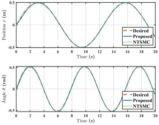
Figure 4. Joint space trajectory tracking performance for axial position (top) and manipulator angle (bottom).

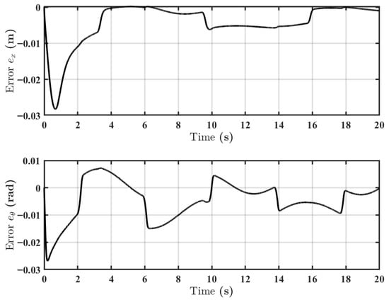
Figure 5. Tracking errors for axial position (top) and manipulator angle (bottom).

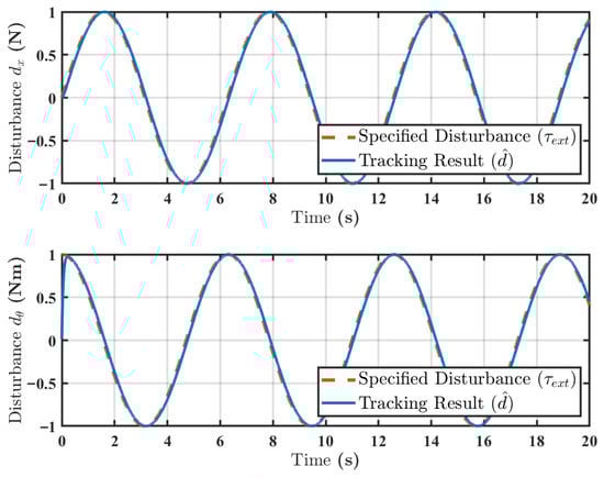
Figure 6. Performance of the disturbance observer in tracking the specified external disturbance ${\tau }_{ext}(t)$.

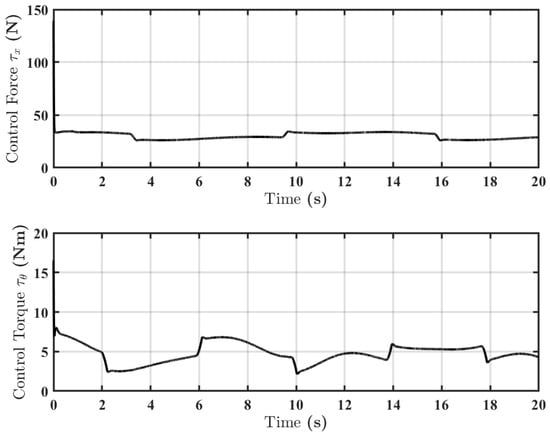
Figure 7. Control inputs: axial force (top) and joint torque (bottom).

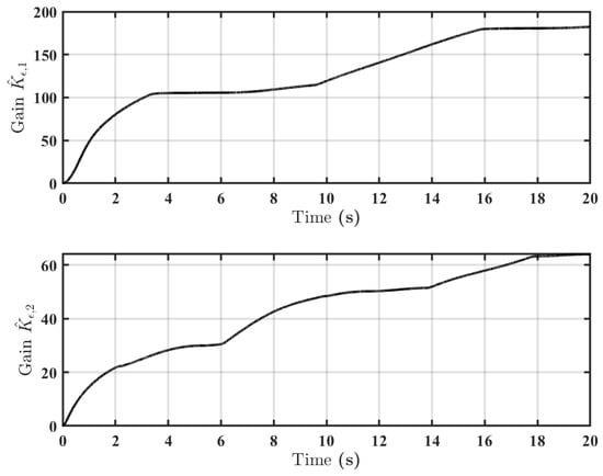
Figure 8. Time history of the adaptive gains ${\widehat{K}}_{ϵ,1}$ (top) and ${\widehat{K}}_{ϵ,2}$ (bottom).

Figure 4 shows the trajectory tracking performance for both the axial position ($x$) and the manipulator angle ($\theta$). It is visually apparent that the actual trajectories (solid blue lines) closely follow the desired paths (dashed red lines), demonstrating the fundamental effectiveness of the control law. As shown in Figure 4, while both methods are capable of tracking the desired trajectory, the “Method in [15]” (dotted green line) exhibits a noticeably larger tracking error and a slower transient response, particularly at the 5 s and 10 s mark where the reference velocity changes direction. In contrast, our proposed method (solid blue line) demonstrates superior precision and robustness, maintaining a significantly tighter tracking performance throughout the simulation. This comparison validates the effectiveness of our integrated framework in handling the compound uncertainties.

A more detailed quantitative analysis is provided by the tracking errors shown in Figure 5. The controller achieves rapid convergence and high steady-state accuracy. For the axial motion, the error settles within a $\pm 0.01$ m tolerance band in just 0.35 s, with the steady-state error (for $t>15$ s) maintained below $1.5\times {10}^{-4}$ m. The manipulator angle exhibits similar performance, converging within a $\pm 0.01$ rad tolerance in 0.42 s, and its steady-state error is confined to $3.2\times {10}^{-4}$ rad. These low error magnitudes quantitatively confirm the controller’s ability to achieve high-precision tracking despite significant uncertainties.

Figure 6 presents the evaluation of the disturbance observer. As configured with a low gain of $L=\mathrm{diag}([2,2])$, the observer’s output $\widehat{d}(t)$ (solid blue line) tracks the specified disturbance ${\tau }_{ext}(t)$ (dashed red line) with noticeable attenuation and phase lag. Quantitatively, the peak amplitude of the estimated disturbance is only about 0.69 N for the axial channel (compared to the target of 1.0 N). This result intentionally demonstrates the direct trade-off between observer gain and tracking bandwidth; while a low gain ensures stability, it limits the ability to track fast-varying signals, leaving the residual portion of the disturbance to be handled by the adaptive robust term of the NTSMC.

The control inputs are shown in Figure 7. The axial force and joint torque are smooth and continuous, confirming that the boundary layer technique effectively mitigates chattering. The inputs remain well within the predefined saturation limits of $\pm 100$ N and $\pm 50$ Nm.

Finally, Figure 8 illustrates the evolution of the adaptive gains. The gains, ${\widehat{K}}_{ϵ,1}$ and ${\widehat{K}}_{ϵ,2}$, increase initially to counteract the system’s uncertainties and then converge to stable, finite values as the tracking error diminishes. This behavior confirms that the adaptive law effectively adjusts the control effort to the required level without causing unbounded gain growth, thereby ensuring the stability of the closed-loop system.

In summary, the simulation results quantitatively confirm that the proposed adaptive robust controller guarantees high-precision trajectory tracking with rapid convergence. The controller effectively handles parametric uncertainties, friction, and external disturbances, maintaining steady-state errors on the order of ${10}^{-4}$ m/rad while ensuring smooth control action.

6. Conclusions

This paper successfully developed a robust adaptive control framework to address the high-precision tracking problem for pipe inspection robots under significant dynamic uncertainties. We proposed a hierarchical architecture that integrates a finite-time disturbance observer with an adaptive non-singular terminal sliding mode controller. This synergistic design ensures finite-time convergence of tracking errors by actively compensating for lumped disturbances and adapting to parametric uncertainties, all without requiring prior knowledge of the uncertainty bounds. Simulation results validated the controller’s superior tracking accuracy and effective chattering suppression.

Future work will prioritize three key directions: (1) experimental validation of the algorithm on a physical prototype; (2) extension of the framework to more complex multi-DOF robots; and (3) integration with learning-based methods to further enhance the system’s autonomy and adaptability.

References

- Shen, Z.; Xie, M.; Song, Z.; Bao, D. Design and Performance Analysis of a Parallel Pipeline Robot. Electronics 2024, 13, 4848. [Google Scholar] [CrossRef]
- Xie, Q.; Liu, Q. Application of TRIZ Innovation Method to In-Pipe Robot Design. Machines 2023, 11, 912. [Google Scholar] [CrossRef]
- Liu, Q.; Li, C.; Wang, G.; Li, L.; Wang, J.; Tan, J.; Wu, Y. Development of a Pipeline-Cleaning Robot for Heat-Exchanger Tubes. Electronics 2025, 14, 2321. [Google Scholar] [CrossRef]
- Lu, D.; Zhang, Y.; Gong, Z.; Wu, T. A slam method based on multi-robot cooperation for pipeline environments underground. Sustainability 2022, 14, 12995. [Google Scholar] [CrossRef]
- Yin, X.; Pan, L.; Cai, S. Robust adaptive fuzzy sliding mode trajectory tracking control for serial robotic manipulators. Robot. Comput.-Integr. Manuf. 2021, 72, 101884. [Google Scholar] [CrossRef]
- Brunke, L.; Greeff, M.; Hall, A.W.; Yuan, Z.; Zhou, S.; Panerati, J.; Schoellig, A.P. Safe learning in robotics: From learning-based control to safe reinforcement learning. Annu. Rev. Control Robot. Auton. Syst. 2022, 5, 411–444. [Google Scholar] [CrossRef]
- Shao, X.; Zhang, J.; Zhang, W. Distributed cooperative surrounding control for mobile robots with uncertainties and aperiodic sampling. IEEE Trans. Intell. Transp. Syst. 2022, 23, 18951–18961. [Google Scholar] [CrossRef]
- Wu, J.; Jin, Z.; Liu, A.; Yu, L.; Yang, F. A survey of learning-based control of robotic visual servoing systems. J. Frankl. Inst. 2022, 359, 556–577. [Google Scholar] [CrossRef]
- Hassan, N.; Saleem, A. Neural network-based adaptive controller for trajectory tracking of wheeled mobile robots. IEEE Access 2022, 10, 13582–13597. [Google Scholar] [CrossRef]
- Wu, L.; Liu, J.; Vazquez, S.; Vazquez, S.; Mazumder, S.K. Sliding mode control in power converters and drives: A review. IEEE/CAA J. Autom. Sin. 2021, 9, 392–406. [Google Scholar] [CrossRef]
- Mousavi, Y.; Bevan, G.; Kucukdemiral, I.B.; Fekih, A. Sliding mode control of wind energy conversion systems: Trends and applications. Renew. Sustain. Energy Rev. 2022, 167, 112734. [Google Scholar] [CrossRef]
- Feng, H.; Song, Q.; Ma, S.; Ma, W.; Yin, C.; Cao, D.; Yu, H. A new adaptive sliding mode controller based on the RBF neural network for an electro-hydraulic servo system. ISA Trans. 2022, 129, 472–484. [Google Scholar] [CrossRef]
- Yao, D.; Li, H.; Shi, Y. Event-based average consensus of disturbed MASs via fully distributed sliding mode control. IEEE Trans. Autom. Control 2023, 69, 2015–2022. [Google Scholar] [CrossRef]
- Liu, M.; Xu, N.; Wang, H.; Zong, G.; Zhao, X.; Li, L. Hierarchical non-singular terminal sliding mode control for constrained under-actuated nonlinear systems against sensor faults. Nonlinear Dyn. 2025, 113, 16913–16929. [Google Scholar] [CrossRef]
- Guo, K.; Shi, P.; Wang, P.; He, C.; Zhang, H. Non-singular terminal sliding mode controller with nonlinear disturbance observer for robotic manipulator. Electronics 2023, 12, 849. [Google Scholar] [CrossRef]
- Xu, B.; Zhang, L.; Ji, W. Improved non-singular fast terminal sliding mode control with disturbance observer for PMSM drives. IEEE Trans. Transp. Electrific. 2021, 7, 2753–2762. [Google Scholar] [CrossRef]
- Gil, J.; You, S.; Lee, Y.; Kim, W. Nonlinear sliding mode controller using disturbance observer for permanent magnet synchronous motors under disturbance. Expert Syst. Appl. 2023, 214, 119085. [Google Scholar] [CrossRef]
- Zhang, Y.; Edwards, C.; Belmont, M.; Li, G. Robust model predictive control for constrained linear system based on a sliding mode disturbance observer. Automatica 2023, 154, 111101. [Google Scholar] [CrossRef]
- Wang, H.; Zhang, Y.; Zhao, Z.; Tang, X.; Yang, J.; Chen, I.-M. Finite-time disturbance observer-based trajectory tracking control for flexible-joint robots. Nonlinear Dyn. 2021, 106, 459–471. [Google Scholar] [CrossRef]
- Vo, A.T.; Truong, T.N.; Kang, H.J. A novel tracking control algorithm with finite-time disturbance observer for a class of second-order nonlinear systems and its applications. IEEE Access 2021, 9, 31373–31389. [Google Scholar] [CrossRef]
- Huang, D.; Huang, T.; Qin, N.; Li, Y.; Yang, Y. Finite-time control for a UAV system based on a finite-time disturbance observer. Aerosp. Sci. Technol. 2022, 129, 107825. [Google Scholar] [CrossRef]
- Li, T.; Liu, X.; Yu, H. Backstepping nonsingular terminal sliding mode control for PMSM with finite-time disturbance observer. IEEE Access 2021, 9, 135496–135507. [Google Scholar] [CrossRef]
- Fu, C.; Zhang, C.; Zhang, G.; Song, J.; Zhang, C.; Duan, B. Disturbance observer-based finite-time control for three-phase AC–DC converter. IEEE Trans. Ind. Electron. 2021, 69, 5637–5647. [Google Scholar] [CrossRef]
- Fei, J.; Liu, L.; Chen, Y. Finite-time disturbance observer of active power filter with dynamic terminal sliding mode controller. IEEE J. Emerg. Sel. Top. Power Electron. 2022, 11, 1604–1615. [Google Scholar] [CrossRef]
- Zhang, D.; Hu, J.; Cheng, J.; Wu, Z.-G.; Yan, H. A novel disturbance observer based fixed-time sliding mode control for robotic manipulators with global fast convergence. IEEE/CAA J. Autom. Sin. 2024, 11, 661–672. [Google Scholar] [CrossRef]
- Derakhshannia, M.; Moosapour, S.S. Disturbance observer-based sliding mode control for consensus tracking of chaotic nonlinear multi-agent systems. Math. Comput. Simul. 2022, 194, 610–628. [Google Scholar] [CrossRef]
- Yang, T.; Deng, Y.; Li, H.; Sun, Z.; Cao, H.; Wei, Z. Fast integral terminal sliding mode control with a novel disturbance observer based on iterative learning for speed control of PMSM. ISA Trans. 2023, 134, 460–471. [Google Scholar] [CrossRef]
Disclaimer/Publisher’s Note: The statements, opinions and data contained in all publications are solely those of the individual author(s) and contributor(s) and not of MDPI and/or the editor(s). MDPI and/or the editor(s) disclaim responsibility for any injury to people or property resulting from any ideas, methods, instructions or products referred to in the content. |
© 2025 by the authors. Licensee MDPI, Basel, Switzerland. This article is an open access article distributed under the terms and conditions of the Creative Commons Attribution (CC BY) license (https://creativecommons.org/licenses/by/4.0/).