Symmetric UAV Cooperative Lifting Motion Planning in Confined Space

Abstract

This paper investigates the motion planning problem for symmetric UAV cooperative lifting in confined spaces. A dynamic model of the symmetric UAV cooperative lifting system is established, and differential flatness analysis is employed to transform nonlinear dynamics into constraints on flat outputs, thereby simplifying the motion planning process. The planning framework consists of two levels: path planning and trajectory planning. For path planning, a reinforcement learning-based bidirectional RRT (RLDB-BiRRT) method is proposed, which integrates the random tree expansion mechanism with the DDPG algorithm to achieve adaptive directional bias. This approach effectively mitigates the issues of low search efficiency and excessive redundant nodes inherent in traditional RRT algorithms. For trajectory planning, an adaptive safe flight corridor (SFC) construction method is introduced, combining symmetric ellipsoids and convex polyhedra to generate high-quality linear constraints. Building upon the proposed motion planning method and leveraging differential flatness analysis, a unified planning framework is developed that seamlessly integrates the reinforcement learning-enhanced path planning with adaptive safe corridor construction and differential-flatness-based trajectory optimization, specifically designed for symmetric UAV cooperative lifting tasks in confined spaces. This integrated approach enhances corridor space utilization and ensures trajectory continuity. Simulation experiments validate the effectiveness of the proposed methods, demonstrating their capability to generate dynamically feasible, smooth, and safe transportation trajectories in confined environments, while effectively constraining load swing and UAV attitude angles. This study provides theoretical foundations and practical references for the application of symmetric UAV cooperative lifting in low-altitude logistics and emergency transportation scenarios.

1. Introduction

Low-altitude logistics, an innovative domain emerging from the integration of the low-altitude economy and smart logistics, effectively utilizes low-altitude Unmanned Aerial Vehicles (UAV) to overcome ground transportation constraints. It not only reduces operational costs but also demonstrates significant value in specialized applications such as emergency rescue, medical supply delivery, and oversized cargo transport. Quadrotor UAV are commonly deployed in these scenarios; however, limited payload capacity of individual drones has led to the development of cooperative transportation using symmetric drone formations. When operating in confined spaces, these systems encounter challenges such as spatial constraints, complex terrain, and obstacles that impede movement. To ensure safe and smooth navigation through such environments, motion planning that incorporates UAV dynamics is essential.

Motion planning consists of two levels: path planning and trajectory planning. Path planning identifies a collision-free geometric path in a constrained space, often by simplifying the system as a point mass. Trajectory planning further incorporates dynamic configuration and temporal constraints to generate a time-parameterized executable trajectory. Among various path planning algorithms, sampling-based methods such as the Rapidly-exploring Random Tree (RRT) are widely used. RRT incrementally expands tree nodes toward the goal, offering advantages like short planning times and adaptability to high-dimensional environments. However, it often produces suboptimal paths due to random sampling and exhibits low search efficiency. Improved variants such as RRT* guarantee asymptotic optimality by rewiring the tree, and Informed RRT* further accelerates convergence by heuristically constraining the sampling domain. Recent hybrids couple RRT* with complementary techniques: an adaptive RRT* was fused with the Dynamic Window Approach [1] to enhance dynamic feasibility, and a bidirectional RRT integrated with particle-swarm optimization [2] was proposed for smoother trajectories. Nevertheless, their efficacy in highly confined spaces remains limited.

In the field of trajectory planning, many remarkable solutions have emerged. Alkomy et al. [3] used polynomial trajectories for vibration reduction of a quadrotor with a cable-suspended payload. Quadratic programming (QP) approaches reformulate trajectory generation into problems with linear constraints [4] or mixed-integer quadratic programming (MIQP) formulations [5], both demonstrating strong performance in complex scenarios. Reinforcement learning (RL) methods generate trajectories via value function approximation and have shown robustness in varying conditions [6,7]. The challenge of real-time obstacle avoidance in dense environments has been addressed through an integrated sensor-based planning approach [8].

While these studies provide a foundation for cooperative trajectory planning, symmetric dual-drone systems introduce additional challenges. Planning must account for both individual drone dynamics and inter-agent coordination. Differential flatness simplifies this by reducing the high-dimensional system into smooth parameterizations of flat outputs, embedding dynamics into the outputs and their derivatives. The challenge of multi-helicopter cooperative transportation in crowded environments has been addressed through real-time trajectory planning leveraging differential flatness [9]. In multi-UAV systems, Valentim et al. [10] introduced a new set of flat outputs for cooperative load transport, achieving precise tracking.

Safe Flight Corridors (SFC) compress the search space into finite-dimensional representations, providing convex constraints for trajectory optimization. Various SFC construction methods have been proposed, including point-cloud processing techniques [11,12] and convex optimization-based approach [13]. Common representations include spherical corridors [14] and ellipsoidal corridors [15]. However, these methods often model drones as point masses, neglecting formation constraints in cooperative systems.

To enhance the adaptability of path planning while accounting for the formation constraints of a symmetric UAV cooperative lifting system in confined spaces, this paper proposes a motion planning strategy comprising the following components: (1) A novel integration of DDPG reinforcement learning with a bidirectional RRT framework (RLDB-BiRRT) is introduced, which significantly improves path search efficiency through adaptive parameter tuning. (2) An adaptive safe flight corridor construction method is designed, which enhances the spatial utilization of cooperative systems by hybridizing ellipsoidal and polyhedral geometries, thereby addressing a key challenge long overlooked by safe flight corridor methods—the configuration constraints of UAV formations. (3) A unified planning framework is developed, seamlessly integrating the above reinforcement learning-enhanced path planning method and adaptive safe corridor construction technique with differential-flatness-based trajectory optimization, specifically tailored for symmetric UAV cooperative lifting tasks in confined spaces.

2. Dynamic Model and Analysis

The overall architecture of the symmetric UAV cooperative transportation system is depicted in Figure 1. The process begins with the construction of a grid map of the confined space. A reinforcement learning-based Bi-RRT algorithm then generates a feasible path, followed by the construction of a Safe Flight Corridor (SFC) via convex decomposition. Finally, the optimal trajectory $X_d$ for the controller is obtained by solving an optimization problem.

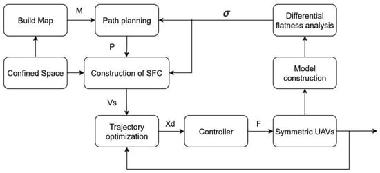
Figure 1. The overall framework of the control system.

Compared to single-UAV transport, the symmetric cooperative system introduces additional degrees of freedom and nonlinear dynamic coupling. This necessitates simultaneous management of both UAVs’ attitudes and thrusts while satisfying geometric and dynamic equilibrium constraints, significantly increasing planning and control complexity. To streamline trajectory planning while ensuring dynamic feasibility, the system’s dynamic model is firstly established. Subsequently, differential flatness analysis is applied, transforming the nonlinear dynamics into equivalent constraints on the flat outputs and their derivatives. This reduces constraint dimensionality and enables efficient analytical motion planning.

2.1. Dynamic Model

The physical model and coordinate system of the symmetric UAV cooperative transportation system are illustrated in Figure 2, where $O-XYZ$ denotes the inertial frame. The positions of the symmetric UAVs, UAV1 and UAV2, are denoted as $(x_1,y_1,z_1)$ and $(x_2,y_2,z_2)$, respectively, and the payload position is denoted as $(x_3,y_3,z_3)$.

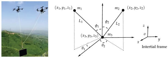
Figure 2. Physical model and coordinate system of the symmetric UAV cooperative lifting system.

The cable lengths connecting UAV1 and UAV2 to the payload are $L_1$ and $L_2$, respectively. The masses of the symmetric UAVs and the payload are $m_1$, $m_2$, and $m_3$, respectively. The angles ${\theta }_1$ and ${\theta }_2$ represent the angles between the projections of cables $L_1$ and $L_2$ onto the $xy$-plane and the x-axis, respectively. The angles ${\varphi }_1$ and ${\varphi }_2$ represent the angles between cables $L_1$, $L_2$ and the z-axis, respectively. Under the thrust generated by their propellers, the UAVs achieve motion control along the X, Y, and Z axes of the inertial frame to accomplish spatial positioning and transportation tasks for the payload.

To facilitate modeling and the design of subsequent algorithms, the following four assumptions are made:

• The UAV fuselage structure is symmetric.
• Both the UAVs and the payload are symmetric rigid bodies with uniform mass density.
• The mass of the cables connecting the UAVs to the payload is negligible.
• The swing angles of the cables connected to the payload satisfy $\varphi ,\theta \in (-{\displaystyle \frac{\pi }{2}},{\displaystyle \frac{\pi }{2}})$.

To derive the dynamic model based on the Lagrange equation, the generalized coordinate vector is introduced:

$$\mathbf{q}={[L_1,{\theta }_1,{\varphi }_1,L_2,{\theta }_2,{\varphi }_2,x_3,y_3,z_3]}^T\in {\mathbb{R}}^9$$

(1)

where $L_1$ and $L_2$ are the cable lengths, ${\theta }_1,{\varphi }_1$ and ${\theta }_2,{\varphi }_2$ are the swing angles of cable 1 and cable 2, and $x_3,y_3,z_3$ are the payload position coordinates.

The symmetric UAVs are interconnected via the payload and cables. The following kinematic relations are considered in the modeling process:

$$x_1=x_3+L_1\sin {\varphi }_1\cos {\theta }_1,y_1=y_3+L_1\sin {\varphi }_1\sin {\theta }_1,z_1=z_3+L_1\cos {\varphi }_1$$

(2)

Due to the symmetry of the UAVs, we have

$$x_2=x_3+L_2\sin {\varphi }_2\cos {\theta }_2,y_2=y_3+L_2\sin {\varphi }_2\sin {\theta }_2,z_2=z_3+L_2\cos {\varphi }_2$$

(3)

The kinetic energy T and potential energy V of the system are given by:

$$T={\displaystyle \frac{1}{2}}\sum _{i=1}^3{m}_i({\dot{x}}_i^2+{\dot{y}}_i^2+{\dot{z}}_i^2),V=\sum _{i=1}^3{m}_{i}g{z}_i$$

(4)

Substituting the kinematic constraints into these expressions yields the Lagrangian of the system:

$$L(\mathbf{q},\dot{\mathbf{q}})=T\left(\dot{\mathbf{q}}\right)-V\left(\mathbf{q}\right)$$

(5)

Considering the generalized forces $\mathbf{Q}$ (which include the UAV thrusts and cable tensions), the equations of motion are derived via the Euler–Lagrange equation:

$${\displaystyle \frac{d}{dt}}\left({\displaystyle \frac{\partial L}{\partial {\dot{q}}_i}}\right)-{\displaystyle \frac{\partial L}{\partial q_i}}=Q_i,(i=1,2,\cdots ,9)$$

(6)

The above dynamic equations can be expressed in matrix form as:

$$\mathbf{M}\left(\mathbf{q}\right)\ddot{\mathbf{q}}+\mathbf{C}(\mathbf{q},\dot{\mathbf{q}})\dot{\mathbf{q}}+\mathbf{G}\left(\mathbf{q}\right)=\mathbf{F}$$

(7)

where $\mathbf{M}\left(\mathbf{q}\right)\in {\mathbb{R}}^{9\times 9}$ is the inertia matrix, $\mathbf{C}(\mathbf{q},\dot{\mathbf{q}})\in {\mathbb{R}}^{9\times 9}$ is the Coriolis and centrifugal matrix, $\mathbf{G}\left(\mathbf{q}\right)\in {\mathbb{R}}^{9\times 1}$ is the gravity vector, and $\mathbf{F}\in {\mathbb{R}}^{9\times 1}$ is the generalized force vector applied to the system. The explicit expressions of the matrix can be found in https://blog.csdn.net/weixin_56678845/article/details/153729276?spm=1001.2014.3001.5502 (accessed on 28 October 2025)

2.2. Differential Flatness Analysis

A system is considered differentially flat if there exists a set of flat outputs such that all states and control inputs can be expressed as algebraic functions of these outputs and their finite-order derivatives [16]. This property transforms the complex, nonlinear system dynamics into an equivalent set of constraints on the flat outputs, significantly simplifying trajectory planning.

For the symmetric dual-UAV cooperative transport system studied in this paper, under the assumption that the payload is a point mass, the following vector is selected as the flat output:

$$\mathit{\sigma }={[x_3,y_3,z_3,\varphi ]}^T$$

(8)

where $x_3,y_3,z_3$ are the coordinates of the payload’s center of mass in the inertial frame, and $\varphi$ is a common cable inclination angle, embodying the symmetric condition ${\varphi }_1={\varphi }_2=\varphi$.

The differential flatness is established by demonstrating that all generalized coordinates $\mathbf{q}$ (from Equation (1)) and the generalized forces F in the system’s Lagrangian dynamics (Equation (7)) can be algebraically expressed using $\mathit{\sigma }$ and its derivatives.

The components of the generalized coordinate vector $\mathbf{q}$ are expressed in terms of the flat outputs as follows. The payload coordinates $x_3,y_3,z_3$ are elements of $\mathit{\sigma }$ by definition. The symmetric cable inclination is directly specified: ${\varphi }_1={\varphi }_2=\varphi$.

The horizontal swing angles ${\theta }_1$ and ${\theta }_2$ are determined by the system’s kinematics and dynamics. The system’s symmetry implies that the two UAVs are symmetrically distributed about the payload in the horizontal plane, leading to the relation:

$${\theta }_2={\theta }_1+\pi$$

(9)

To find an algebraic expression for ${\theta }_1$, we analyze the payload’s dynamics. The force balance equations for the payload in the horizontal plane, which are inherent in the structure of the Lagrangian model, are:

$$\begin{array}{cc}\hfill m_3{\ddot{x}}_3& =T_1\sin \varphi \cos {\theta }_1+T_2\sin \varphi \cos {\theta }_2\hfill \end{array}$$

(10)

$$\begin{array}{cc}\hfill m_3{\ddot{y}}_3& =T_1\sin \varphi \sin {\theta }_1+T_2\sin \varphi \sin {\theta }_2\hfill \end{array}$$

(11)

Substituting the geometric constraint ${\theta }_2={\theta }_1+\pi$ (i.e., $\cos {\theta }_2=-\cos {\theta }_1,\sin {\theta }_2=-\sin {\theta }_1$) into Equations (10) and (11) yields:

$$\begin{array}{cc}\hfill m_3{\ddot{x}}_3& =(T_1-T_2)\sin \varphi \cos {\theta }_1\hfill \end{array}$$

(12)

$$\begin{array}{cc}\hfill m_3{\ddot{y}}_3& =(T_1-T_2)\sin \varphi \sin {\theta }_1\hfill \end{array}$$

(13)

In the ideally symmetric configuration corresponding to either stationary conditions or uniform linear motion, the cable tensions satisfy $T_1=T_2$. However, the presence of horizontal load acceleration breaks this tension symmetry ($T_1\ne T_2$) to enable coordinated system motion, thereby producing the control moment essential for manipulating the load’s dynamic state.

A more rigorous approach involves solving for ${\theta }_1$ directly from the horizontal force balance. For the system to generate horizontal acceleration, a non-zero control moment is required, which implies $T_1\ne T_2$. Under this condition, dividing Equation (13) by Equation (12) cancels out the common factor $(T_1-T_2)\sin \varphi$, yielding:

$${\displaystyle \frac{{\ddot{y}}_3}{{\ddot{x}}_3}}={\displaystyle \frac{\sin {\theta }_1}{\cos {\theta }_1}}=\tan {\theta }_1$$

(14)

Therefore, provided a horizontal acceleration exists $({\ddot{x}}_3,{\ddot{y}}_3)\ne (0,0)$, the horizontal swing angle ${\theta }_1$ is determined by the algebraic relation:

$${\theta }_1=arctan2({\ddot{y}}_3,{\ddot{x}}_3)$$

(15)

This crucial equation links ${\theta }_1$ directly to the second-order derivatives of the flat outputs $x_3$ and $y_3$. Consequently, ${\theta }_2={\theta }_1+\pi$.

The cable lengths $L_1$ and $L_2$ are treated as known system parameters, held constant at $L_1=L_2=L_0$ during transport.

With all components of $\mathbf{q}$ now expressed as functions of $\mathit{\sigma }$ and its derivatives, the generalized velocities $\dot{\mathbf{q}}\left(t\right)$ and accelerations $\ddot{\mathbf{q}}\left(t\right)$ are likewise determined.

The final step is to show that the generalized forces F in Equation (7) are also algebraic functions of the flat outputs. Substituting the fully parameterized expressions $\mathbf{q}\left(\mathit{\sigma }\right)$, $\dot{\mathbf{q}}(\mathit{\sigma },\dot{\mathit{\sigma }})$, and $\ddot{\mathbf{q}}(\mathit{\sigma },\dot{\mathit{\sigma }},\ddot{\mathit{\sigma }})$ into the Lagrangian dynamics transforms the differential equation into an identity that algebraically defines F:

$$F=M(\mathit{\sigma },\dot{\mathit{\sigma }},\dots )\ddot{\mathbf{q}}(\mathit{\sigma },\dot{\mathit{\sigma }},\ddot{\mathit{\sigma }})+C(\mathit{\sigma },\dot{\mathit{\sigma }},\dots )\dot{\mathbf{q}}(\mathit{\sigma },\dot{\mathit{\sigma }},\ddot{\mathit{\sigma }})+G\left(\mathit{\sigma }\right)$$

(16)

The physical control inputs—the UAV thrust vectors ${\mathbf{F}}_1,{\mathbf{F}}_2$ and the cable tensions $T_1,T_2$—are linearly related to specific components of this generalized force vector F. For example, the components of F corresponding to the swing angles in the Lagrangian formulation are directly related to the moments generated by the cable tensions. The UAV thrusts can subsequently be resolved from the force balance in their respective translational dynamics, where all other terms (position, tension) are already known functions of $\mathit{\sigma }$. This completes the proof that all states and inputs are algebraically parameterized by the flat output.

The symmetric dual-UAV cooperative lifting system is differentially flat with the flat output $\mathit{\sigma }={[x_3,y_3,z_3,\varphi ]}^T$. This property allows the complex motion planning problem to be reduced to planning within the flat output space. A trajectory for $\mathit{\sigma }\left(t\right)$ automatically defines a dynamically feasible trajectory for the full system, guaranteed by the algebraic consistency with the Lagrangian model. This forms the theoretical foundation for the minimum-snap trajectory optimization presented in Section 5.

3. Path Planning with Reinforcement Learning

3.1. Directional-Biased Bidirectional RRT

The directional-biased bidirectional RRT (DB-BiRRT) algorithm builds upon our prior work [17], where the core framework was initially developed and validated. In this paper, we focus on its application to the symmetric UAV cooperative system. The algorithm integrates goal-biased sampling, improved potential field guidance, and adaptive step size to optimize path planning in confined spaces.

3.1.1. Goal-Biased Mechanism with Regional Probability Sampling

The algorithm employs an adaptive goal-biasing strategy to balance exploration and exploitation:

$$P_{\mathrm{bias}}=\left\{\begin{array}{cc}{P}_{\mathrm{direct}},\hfill & \mathrm{if}r\le P_0\hfill \\ P_{\mathrm{regional}},\hfill & \mathrm{if}r>P_0\hfill \end{array}\right.$$

(17)

where $P_{\mathrm{direct}}$ denotes the target point coordinates, $P_{\mathrm{regional}}$ represents the coordinates of a regional probability cluster point, $P_0$ is the bias probability threshold, and $r\in (0,1)$ is a random number.

When $r>P_0$, sampling is based on a regional probability distribution determined by a Gaussian function:

$$G\left(d\right)=exp\left[-{\displaystyle \frac{1}{2}}{\left({\displaystyle \frac{d}{\zeta }}\right)}^2\right]$$

(18)

where $\zeta =kL$ is the standard deviation proportional to the start-target distance L, k is a scaling factor, and d is the perpendicular distance from a region’s center to the start-target line.

3.1.2. Direction Guidance Mechanism Based on Improved Potential Field

To address local minima in traditional potential fields, we introduce an improved potential field that incorporates random sampling points. The potential functions are defined as:

$$\begin{array}{cccc}\hfill U_{\mathrm{att}}\left(q\right)& =\left\{\begin{array}{cc}{\displaystyle \frac{1}{2}}{\alpha }_1{d}_g{(q,q_{\mathrm{goal}})}^2,\hfill & d_g<d_{g0}\hfill \\ {\displaystyle \frac{1}{2}}{\alpha }_1{d}_{g0}{d}_g(q,q_{\mathrm{goal}}),\hfill & d_g\ge d_{g0}\hfill \end{array}\right.\hfill & \hspace{1em}\hspace{1em}\hspace{1em}& \hspace{1em}\hspace{1em}\hspace{1em}\hspace{1em}\end{array}$$

(19)

$$\begin{array}{cc}\hfill U_{\mathrm{rep}}\left(q\right)& =\left\{\begin{array}{cc}{\displaystyle \frac{1}{2}}\beta {\left({\displaystyle \frac{1}{d(q,q_{\mathrm{obs}})}}-{\displaystyle \frac{1}{d_0}}\right)}^2{d}_g{(q,q_{\mathrm{goal}})}^n,\hfill & d(q,q_{\mathrm{obs}})<d_0\hfill \\ 0,\hfill & d(q,q_{\mathrm{obs}})\ge d_0\hfill \end{array}\right.\hfill \end{array}$$

(20)

where ${\alpha }_1$ and ${\alpha }_2$ are attractive gain coefficients; $\beta$ is the repulsive gain coefficient; q, $q_{\mathrm{obs}}$, $q_{\mathrm{goal}}$ are the coordinates of the current node, obstacle, and target point; $d(q,q_{\mathrm{obs}})$, $d_g(q,q_{\mathrm{goal}})$ are Euclidean distances; $d_0$ is the maximum influence distance of obstacles; $d_{g0}$ is the threshold distance for the attractive field; n is the repulsive strength parameter ($n>0$).

The corresponding forces are derived as:

$$\begin{array}{ccccc}\hfill F_{\mathrm{att}}& =-\nabla U_{\mathrm{att}}\left(q\right)=\left\{\begin{array}{cc}{\alpha }_1{d}_g(q,q_{\mathrm{goal}}),\hfill & d_g<d_{g0}\hfill \\ {\alpha }_1{d}_{g0},\hfill & d_g\ge d_{g0}\hfill \end{array}\right.\hfill & \hspace{1em}\hspace{1em}\hspace{1em}\hspace{1em}& \hspace{1em}\hspace{1em}\hspace{1em}\hspace{1em}& \hspace{1em}\hspace{1em}\hspace{1em}\hspace{1em}\end{array}$$

(21)

$$\begin{array}{cc}\hfill F_{\mathrm{rep}}& =-\nabla U_{\mathrm{rep}}\left(q\right)=\left\{\begin{array}{cc}\beta \left({\displaystyle \frac{1}{d(q,q_{\mathrm{obs}})}}-{\displaystyle \frac{1}{d_0}}\right){\displaystyle \frac{d_g{(q,q_{\mathrm{goal}})}^n}{d{(q,q_{\mathrm{obs}})}^2}}{\displaystyle \frac{\partial d(q,q_{\mathrm{obs}})}{\partial q}},\hfill & d(q,q_{\mathrm{obs}})<d_0\hfill \\ 0,\hfill & d(q,q_{\mathrm{obs}})\ge d_0\hfill \end{array}\right.\hfill \end{array}$$

(22)

The direction of $F_{\mathrm{att}}$ is from the current node toward the target, while $F_{\mathrm{rep}}$ is directed from the obstacle toward the current node.

3.1.3. Adaptive Step Size Mechanism

An adaptive step size based on obstacle density enhances planning flexibility:

$$L=L_{\min }+(L_{\max }-L_{\min })e^{-k·\rho }$$

(23)

where $\rho =A_{\mathrm{obs}}/A_{\mathrm{total}}$ is the obstacle density ratio, $A_{\mathrm{total}}$ is the area of the obstacle detection region, $A_{\mathrm{obs}}$ is the area occupied by obstacles, $L_{\max }$ and $L_{\min }$ are the step size bounds, and k is a decay coefficient.

These adaptive parameters $P_0$, $\beta$, and L are dynamically optimized by the reinforcement learning module described in the next subsection.

3.2. Reinforcement Learning Supporting

To enhance the adaptability and flexibility of the algorithm in environments of varying complexity, this paper proposes a reinforcement learning-supported DB-BiRRT (RLDB-BiRRT) method, which integrates a learning module to dynamically generate key parameters during node expansion. The overall framework is illustrated in Figure 3.

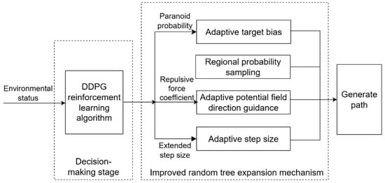
Figure 3. The framework of RLDB-BiRRT.

With the reinforcement learning support, the adaptive parameters $P_0$ (target bias probability), $\beta$ (repulsive gain coefficient), and L (step size) in Equations (17), (22), and (23) are dynamically output by a trained decision-making model. The random tree expansion process is modeled as a Markov Decision Process (MDP), with the following components.

3.2.1. State Space

To capture sufficient environmental information around a node, the state space is designed as:

$$S=\{{\mathbf{D}}_{g1},{\mathbf{D}}_{g2},{\mathbf{D}}_{g3},{\mathbf{D}}_{s1},{\mathbf{D}}_{s2},{\mathbf{D}}_{s3},{\mathbf{D}}_{o1},{\mathbf{D}}_{o2},{\mathbf{D}}_{o3},N_{p1},N_{p2},N_{p3}\}$$

(24)

where ${\mathbf{D}}_{gi}$, ${\mathbf{D}}_{si}$, ${\mathbf{D}}_{oi}$ and $N_{pi}$ represent, respectively, the 3D vectors from the current node of tree i to its corresponding target point, to the nearest random sampling point, and to the nearest obstacle, as well as the total number of nodes within a specified radius of the current node of tree i, for $i=1,2,3$.

3.2.2. Action Space

Based on the design and parameter requirements of RLDB-BiRRT, the action space is defined as a continuous vector:

$$A=\{P_{b1},P_{b2},{\beta }_1,{\beta }_2,L_1,L_2\}$$

(25)

where $P_{b1},P_{b2}$: Goal-Biased probabilities for the two trees; ${\beta }_1,{\beta }_2$: Repulsive gain coefficients for the two trees; $L_1,L_2$: Step sizes for the two trees.

3.2.3. Reward Function

The reward function is designed to guide the agent through sparse reward challenges by combining multiple objectives. The four core reward components, their design objectives, triggering conditions, and values are defined in Table 1.

Table 1. Design of fundamental reward components.

Component	Design Objective	Condition	Value
$R_{\mathrm{obs}}$	Penalize proximity to obstacles for safety.	$d_{\mathrm{obs}}<d_{\mathrm{safe}}$	$-1$
		Otherwise	0
$R_{\mathrm{prox}}$	Encourage progress toward the goal.	$d_{\mathrm{goal}}>d_s$	$-1$
		Otherwise	0
$R_{\mathrm{conn}}$	Highly reward successful path connection.	Trees connect	$+100$
		Connection fails	$-200$
$R_{\mathrm{qual}}$	Incentivize shorter paths.	$X<X_{\min }$	$+80$
		$X>X_{\max }$	$-80$
		Otherwise	0

The total reward $R_{\mathrm{total}}$ is formulated as a weighted sum of these components:

$$R_{\mathrm{total}}=w_{\mathrm{obs}}{R}_{\mathrm{obs}}+w_{\mathrm{prox}}{R}_{\mathrm{prox}}+w_{\mathrm{conn}}{R}_{\mathrm{conn}}+w_{\mathrm{qual}}{R}_{\mathrm{qual}}$$

(26)

with the weight coefficients set as: $w_{\mathrm{obs}}=w_{\mathrm{prox}}=w_{\mathrm{conn}}=1.0$ and $w_{\mathrm{qual}}=0.8$, to prioritize safety and feasibility over path optimality.

This hierarchical design prioritizes task success and safety. The primary weights on $R_{\mathrm{obs}}$, $R_{\mathrm{prox}}$, and $R_{\mathrm{conn}}$ ensure the agent first learns a feasible and safe policy, while the secondary weight on $R_{\mathrm{qual}}$ refines the solution for optimality, leading to more stable training.

3.2.4. Training Process

The Deep Deterministic Policy Gradient (DDPG) algorithm [18] is employed to train the agent due to its suitability for continuous action spaces. The agent is trained over a series of episodes. Each episode terminates upon successful connection of the two trees, collision with an obstacle, or exceeding the maximum number of iterations (set to 2000). Upon completion of training, the trained agent is integrated into the complete workflow of the RLDB-BiRRT algorithm, with the pseudocode shown in Algorithm 1. The algorithm begins by initializing parameters, including start and goal positions, the obstacle map, and the two random trees. The pre-trained agent is then loaded. At each decision step, the agent observes the current state S of the environment and outputs an action vector A. This action vector dynamically sets the parameters for target biasing, repulsive field gain, and step size. Based on these adapted parameters, the algorithm performs goal-biased sampling, regional probability sampling, and calculates the expansion direction using the improved potential field. Combined with the adaptive step size, a new sampling point is determined. This sampling cycle continues until the two random trees successfully connect, yielding a feasible path and completing the path planning process.

Algorithm 1: RLDB-BiRRT: Reinforcement Learning-based Bi-RRT

3.3. Simulation Experiments

Simulation experiments were conducted in MATLAB R2023a on a computer equipped with an Intel i9 CPU and 32 GB RAM, to validate the effectiveness and superiority of the proposed RLDB-BiRRT algorithm in path planning. A custom 3D obstacle map with dimensions of $45\times 45\times 45$ cubic units was constructed, incorporating various obstacle primitives including spheres, cylinders, and cuboids, arranged to form complex regions, narrow passages, and scenarios that mimic challenging real-world confined spaces.

Parameters for the RLDB-BiRRT algorithm were set as follows: obstacle influence distance $d_0=10$ units, attractive field threshold $d_{g0}=50$ units, attractive gains ${\alpha }_1=2,{\alpha }_2=10$, safe distance $d_{\mathrm{safe}}=5$ units, repulsive parameter $n=2$, with adaptive step size bounds $L_{\max }=3.5$ units, $L_{\min }=0.2$ units, and a maximum of 2000 iterations per planning trial. The hyperparameters for the DDPG algorithm, determined through empirical tuning, are listed in Table 2.

Table 2. DDPG algorithm hyperparameters.

Parameter	Value
Actor Learning Rate	0.003
Critic Learning Rate	0.003
Replay Buffer Size	$5\times {10}^4$
Mini-batch Size	128
Initial Noise Std	0.1
Noise Std Decay Rate	0.995
Minimum Noise Std	0.01

The training reward curve of the DDPG agent is shown in Figure 4. It can be observed that the agent’s average reward exhibits considerable variation during the initial exploration phase. As training progresses, the overall trend stabilizes. The reward curve fluctuates within a narrow range after approximately 500 episodes, demonstrating the convergence and improved stability of the training process.

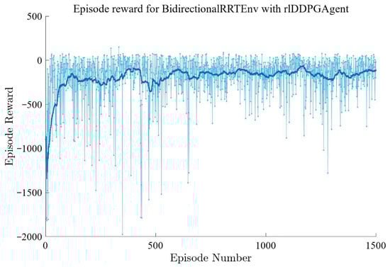
Figure 4. Training reward curve of the DDPG agent.

To evaluate the performance of the RLDB-BiRRT algorithm, three benchmark sampling-based algorithms were selected for comparison: the classic RRT* [19], Improved Bi-RRT* [20], and APF-RRT* [21]. These algorithms were tested on identical obstacle maps to ensure a fair and comprehensive performance comparison. For all compared algorithms, the maximum number of iterations was set to 2000, with a fixed step size of 1.75 units, a maximum connection distance of 5 units, and a rewiring radius of 5 units for RRT*-based optimizations.

The simulation results of the four algorithms are qualitatively compared in Figure 5. Twenty independent Monte Carlo trials were conducted for each algorithm to ensure statistical significance. The runtime, path length, and number of nodes were recorded for each trial. The statistical results for computation time and path length are summarized in Figure 6 and Figure 7, respectively. The results indicate that the proposed RLDB-BiRRT algorithm achieves a favorable balance between planning efficiency (time) and path quality (length), consistently outperforming the benchmark algorithms in these key metrics across diverse environmental configurations.

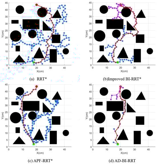
Figure 5. Comparison of paths generated by the four algorithms in a representative scenario.

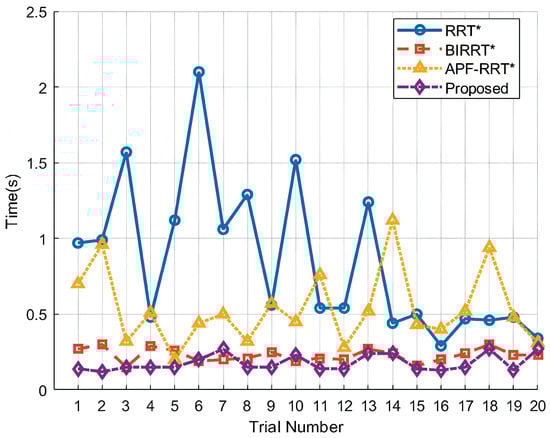
Figure 6. Comparison of average computation time of the four algorithms.

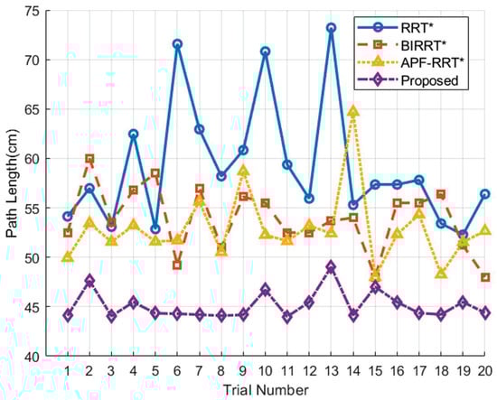
Figure 7. Comparison of average final path length of the four algorithms.

The proposed RLDB-BiRRT algorithm introduces a learning-based paradigm to dynamically adapt the core expansion parameters of a BiRRT, aiming for greater robustness and efficiency across diverse environments. We note that deep reinforcement learning comprises both offline training and online inference phases. The former is computationally intensive and time-consuming, as it requires extensive environmental interactions and experience replay. However, once training is completed, the computational overhead of online inference—that is, using the trained model to make decisions based on the current state—becomes very low. Each inference step takes approximately 0.08 seconds and consumes 0.315 MB of memory. Such a computational load is considered typical for conventional offline training scenarios. Statistical results show that the agent first discovers a feasible solution within 184 ± 27 episodes and reaches a reward plateau (±5 %) after approximately 487 ± 42 episodes. The entire training process takes 21.6 min. During online execution, the average decision time is only 0.18 s, which meeting the fast-response requirement.

4. Safe Flight Corridor Construction

For symmetric UAV systems performing cooperative transportation in confined spaces, the high obstacle density and stringent spatial constraints present dual challenges. Traditional safe flight corridor (SFC) methods addressed in [14,15] typically model free space as spheres or ellipsoids. While these approaches suit single-UAV high-speed flight scenarios, they fail to accommodate the unique configuration requirements of dual-UAV cooperative systems, resulting in poor corridor space utilization and trajectories prone to boundary violations.

To address this issue, this study proposes an adaptive hybrid geometric construction framework. The method begins by optimizing and pruning the raw nodes generated from path planning in Section 3 to extract key waypoints as the basis for corridor segmentation. Subsequently, using each path segment as an axis, it constructs continuous safe flight corridors through adaptive ellipsoid construction and convex polyhedron optimization. Finally, these convex polyhedral constraints are embedded into the trajectory optimization framework, providing high-quality linear constraint spaces for backend planning. This technical approach effectively balances safety, spatial continuity, and utilization efficiency, establishing a reliable trajectory planning foundation for cooperative transportation tasks in confined spaces.

4.1. Path Segmentation and Initial Corridor Generation

The process begins with the piecewise linear path $P=\{P_0,P_1,\cdots ,P_n\}$ generated by the global planner described in Section 3. For each segment $L_i=\{P_i\to P_{i+1}\}$, an initial spherical corridor is constructed. This sphere fully contains both endpoints and the segment’s midpoint, establishing a preliminary collision-free volume for subsequent ellipsoidal refinement.

As illustrated in Figure 8, conventional methods generate an ellipsoidal corridor per path segment, with the overall SFC composed of convex polyhedra derived from the ellipsoids’ tangent planes. Let ${\mathcal{V}}_i$ denote the convex polyhedron for segment $L_i$; the complete corridor is then ${\mathcal{V}}_s=\{{\mathcal{V}}_i\mid i=0,1,\cdots ,n-1\}$. This construction ensures that consecutive polyhedra ${\mathcal{V}}_i$ and ${\mathcal{V}}_{i+1}$ intersect at the shared waypoint $P_{i+1}$, guaranteeing continuity at these critical junctions.

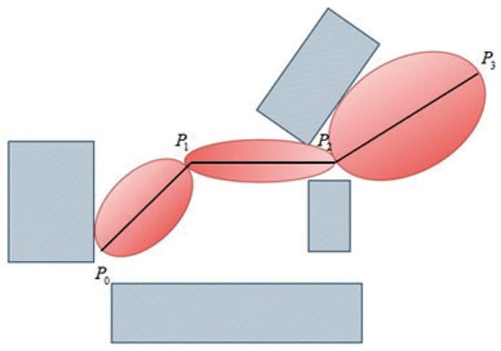
Figure 8. Traditional SFC construction using spheres.

However, these methods typically consider a single UAV. For cooperative lifting, the spatial constraints are coupled. Our proposed adaptive SFC explicitly constructs corridors that accommodate the formation of two UAVs and the suspended payload, thereby improving space utilization.

An ellipsoid is formally defined as:

$$\mathcal{E}=\xi (\mathbf{C},\mathbf{d})=\left\{\mathbf{p}={\mathbf{C}}^T{\mathbf{p}}^{\prime }+\mathbf{d}\mid \parallel {\mathbf{p}}^{\prime }\parallel \le 1\right\}$$

(27)

where $\mathcal{E}$ is the ellipsoid, $\mathbf{C}$ is a $3\times 3$ symmetric positive definite matrix shaping the ellipsoid, and $\mathbf{d}$ is its center. The matrix $\mathbf{C}$ can be decomposed via eigenvalue decomposition as $\mathbf{C}={\mathbf{R}}^T\mathbf{S}\mathbf{R}$.

Here, $\mathbf{R}$ is a rotation matrix aligning the ellipsoid with the global coordinate frame, and $\mathbf{S}=\mathrm{diag}(a,b,c)$ is a diagonal matrix where a, b, and c represent the lengths of the semi-principal axes, with $a\ge b$ and $a\ge c$.

The ellipsoid must fully enclose its corresponding path segment L while remaining free of obstacles O. The process starts by creating a sphere centered at the segment midpoint, $\mathbf{d}=(P_i+P_{i+1})/2$, with initially equal axis lengths.

4.2. Ellipsoid Adaptive Construction

To resolve issues of insufficient obstacle clearance and intersection discontinuity prevalent in initial corridors (Figure 8), we introduce a dual-objective adaptive strategy termed “Dynamic Ellipsoid Adaptation and Intersection Continuity Assurance” as shown in Figure 9 with the procedure is as follows:

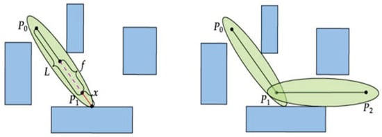
Figure 9. Adaptive elongation of the ellipsoid’s major axis to increase clearance from nearby obstacles.

First, the major axis of the ellipsoid is adaptively adjusted. The segment’s direction vector is $\mathbf{dr}={\displaystyle \frac{P_{i+1}-P_i}{\parallel P_{i+1}-P_i\parallel }}$ For an obstacle point ${\mathbf{P}}_o$, its projection parameter along the segment is $t=({\mathbf{P}}_o-P_i)·\mathbf{dr}$ The corresponding projection point on the segment is: ${\mathbf{P}}_t=P_i+t·\mathbf{dr}$ The perpendicular distance from the obstacle to the segment is then: $d_i=\parallel {\mathbf{P}}_o-{\mathbf{P}}_t\parallel$

If $d_i\le d_{\mathrm{threshold}}$ (e.g., $d_{\mathrm{threshold}}=0.1$), the obstacle is considered influential. The minimum distance from the obstacle to either segment endpoint is computed as:

$$x=min(\parallel {\mathbf{P}}_o-P_i\parallel ,\parallel {\mathbf{P}}_o-P_{i+1}\parallel )$$

(28)

This distance x is used to extend the major axis, enhancing the safety margin. If no obstacle is within the threshold, x is set to a fixed positive increment. The updated scaling matrix becomes:

$$\mathbf{S}=\mathrm{diag}(f+x,f,f)$$

(29)

Following the acquisition of a collision-free ellipsoid $\mathcal{E}$, a convex polyhedron ${\mathcal{V}}_p$ is constructed to provide linear inequality constraints for trajectory optimization. The polyhedron is built iteratively from the obstacle set O and a set of uniformly sampled points $S_{\mathrm{sample}}$ on the ellipsoid’s surface, parameterized by spherical coordinates. These are combined into an extended constraint set $O_{\mathrm{extended}}=O\cup S_{\mathrm{sample}}$.

The iterative construction process as shown in Figure 10 is as follows: While $O_{\mathrm{extended}}$ is non-empty, find the point $p_c\in O_{\mathrm{extended}}$ closest to the ellipsoid center $\mathbf{d}$. A constraining hyperplane H tangent to the ellipsoid at $p_c$ is defined. Its normal vector and offset are given by:

$$\mathbf{a}=2{\mathbf{C}}^{-T}(p_c-\mathbf{d})$$

(30)

$$b={\mathbf{a}}^T{p}_c$$

(31)

This defines the half-space $H=\{p\mid {\mathbf{a}}^{T}p\le b\}$, which is added to ${\mathcal{V}}_p$. For all points $p\in O_{\mathrm{extended}}$, the signed distance to H is computed as $d\left(p\right)={\mathbf{a}}^{T}p-b$. Points satisfying $d\left(p\right)>0$ (i.e., outside H) are retained, updating $O_{\mathrm{extended}}$. This loop continues until $O_{\mathrm{extended}}$ is empty, ensuring all obstacle and sample points are interior to the polyhedron.

Figure 10. Iterative refinement process to ensure the ellipsoid maintains a safe distance from all obstacles while preserving path connectivity.

The final convex polyhedron is the intersection of all generated hyperplanes:

$${\mathcal{V}}_p=\bigcap _i{H}_i=\{p\mid {\mathbf{A}}^{T}p\le \mathbf{b}\}$$

(32)

where columns of $\mathbf{A}$ are the normal vectors ${\mathbf{a}}_i$, and $\mathbf{b}$ contains the corresponding offsets $b_i$. Since the initial ellipsoid $\mathcal{E}$ contains segment L, and ${\mathcal{V}}_p$ is constructed from its tangent planes, it is guaranteed that $L\subset {\mathcal{V}}_p$. The incorporation of surface sample points ensures the polyhedron boundary approximates the ellipsoidal shape, while obstacle exclusion guarantees safety.

The adaptive safe corridor shown in Figure 11 effectively meets the obstacle avoidance requirements in complex environments, ensures the spatial continuity between path segments, and enhances the trajectory safety of the symmetric UAV cooperative transportation system.

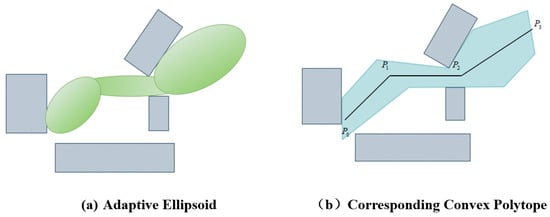
Figure 11. The resulting adaptive safe corridor.

5. Trajectory Planning Based on Safety Corridors

The Safe Flight Corridor (SFC) constructed in Section 4 provides a series of convex polyhedral safe regions, effectively transforming non-convex spatial constraints into manageable linear inequalities. This representation significantly enhances the convergence properties of the trajectory optimization algorithm. By integrating these linear constraints into the planning process, the system guarantees dynamic feasibility and robust obstacle avoidance for the UAV formation within the defined safe space. This section formulates the trajectory generation as a constrained minimum-snap optimization problem, solved via Sequential Quadratic Programming (SQP) to achieve safe, smooth, and controllable flight in complex 3D environments.

5.1. Objective Function Formulation

In trajectory planning for cooperative UAV transportation systems, the minimization of snap is adopted for generating trajectories in confined spaces. This approach ensures continuity in lower-order derivatives (acceleration and jerk), thereby producing smoother motion trajectories, reducing energy consumption, and achieving more manageable control inputs. Furthermore, the minimum-snap optimization problem can be formulated as a quadratic programming (QP) problem, which exhibits lower computational complexity compared to other higher-order optimization methods, making it suitable for real-time applications.

As established in Section 2, the symmetric UAV cooperative transportation system is differentially flat with outputs defined as $\mathit{\sigma }={[x_3,y_3,z_3,\varphi ]}^T$. This property implies that planning trajectories for these flat outputs is sufficient to determine the complete system states and control inputs, thereby significantly simplifying the planning complexity.

The trajectory is represented as an n-th order piecewise polynomial over M segments:

$$\mathbf{p}\left(t\right)=\left\{\begin{array}{cc}{\mathbf{c}}_1^T\mathbf{fi}\left(t\right),\hfill & t_0\le t<t_1\hfill \\ {\mathbf{c}}_2^T\mathbf{fi}\left(t\right),\hfill & t_1\le t<t_2\hfill \\ ⋮\hfill & ⋮\hfill \\ {\mathbf{c}}_M^T\mathbf{fi}\left(t\right),\hfill & t_{M-1}\le t<t_M\hfill \end{array}\right.$$

(33)

where ${\mathbf{c}}_i$ is the coefficient vector for the i-th segment, $\mathbf{fi}\left(t\right)={[1,t,t^2,\dots ,t^n]}^T$ is the polynomial basis vector, and $t_0,t_1,\dots ,t_M$ are the segment time nodes.

The objective is to find the optimal polynomial coefficients that minimize the total snap while satisfying all constraints, formulated as:

$$\begin{array}{cc}\hfill \underset{\mathbf{p}}{min}& f\left(\mathbf{p}\right)=\sum _{i=1}^M{\int }_{t_{i-1}}^{t_i}{∥{\mathbf{p}}_i^{\left(4\right)}\left(t\right)∥}^{2}dt\hfill \\ \hfill \mathrm{s}.\mathrm{t}.& {\mathbf{A}}_{\mathrm{eq}}\mathbf{p}={\mathbf{b}}_{\mathrm{eq}},\hfill \\ \hfill & {\mathbf{A}}_{\mathrm{ineq}}\mathbf{p}\le {\mathbf{b}}_{\mathrm{ineq}}\hfill \end{array}$$

(34)

Here, the objective function $f\left(\mathbf{p}\right)$ minimizes the integral of the squared norm of the snap across all trajectory segments, promoting overall smoothness and energy efficiency.

5.2. Constraints Formulation

5.2.1. Equality Constraints

Equality constraints are imposed to ensure the trajectory satisfies specific state conditions at key points (start, end, and intermediate waypoints) and maintains smooth transitions between segments.For a polynomial segment ${\mathbf{p}}_i\left(t\right)={\mathbf{c}}_i^T\mathbf{fi}\left(t\right)$, the value and derivatives at a specific time $t_0$ can be computed using the basis vector and its derivatives: $\mathbf{fi}\left(t_0\right),\dot{\mathbf{fi}}\left(t_0\right),\ddot{\mathbf{fi}}\left(t_0\right)$, etc. The constraints for position ($p_0$), velocity ($v_0$), and acceleration ($a_0$) at $t_0$ are:

$${\mathbf{c}}_i^T\mathbf{fi}\left(t_0\right)=p_0\left(\mathrm{Pos}\right),{\mathbf{c}}_i^T\dot{\mathbf{fi}}\left(t_0\right)=v_0\left(\mathrm{Vel}\right),{\mathbf{c}}_i^T\ddot{\mathbf{fi}}\left(t_0\right)=a_0\left(\mathrm{Acc}\right)$$

(35)

Similar constraints are applied at intermediate waypoints and the final point to ensure geometric and dynamic consistency.

Continuity between adjacent segments is enforced by equating the derivatives at the connection points. For instance, the continuity of position, velocity, and acceleration between segment i and segment $i+1$ at time $t_i$ is expressed as:

$${\mathbf{c}}_i^T\mathbf{fi}\left(t_i\right)={\mathbf{c}}_{i+1}^T\mathbf{fi}\left(t_i\right)\left(\mathrm{Pos}\right),{\mathbf{c}}_i^T\dot{\mathbf{fi}}\left(t_i\right)={\mathbf{c}}_{i+1}^T\dot{\mathbf{fi}}\left(t_i\right)\left(\mathrm{Vel}\right),{\mathbf{c}}_i^T\ddot{\mathbf{fi}}\left(t_i\right)={\mathbf{c}}_{i+1}^T\ddot{\mathbf{fi}}\left(t_i\right)\left(\mathrm{Acc}\right)$$

(36)

All these linear equality constraints are aggregated into the system ${\mathbf{A}}_{\mathrm{eq}}\mathbf{p}={\mathbf{b}}_{\mathrm{eq}}$.

5.2.2. Inequality Constraints

Inequality constraints are crucial for ensuring the trajectory remains within the Safe Flight Corridor (SFC), thereby guaranteeing safety and obstacle avoidance. A piecewise polynomial trajectory constrained within an SFC.

Each segment i of the trajectory, defined over $[t_i,t_{i+1}]$, is associated with a convex polyhedron ${\mathcal{V}}_i$ from the SFC. This polyhedron is defined by a set of hyperplanes ${\mathcal{V}}_i={\left\{({\mathbf{n}}_{i,j},{\mathbf{q}}_{i,j})\right\}}_{j=1}^{m_i}$, where ${\mathbf{n}}_{i,j}$ is the outward-pointing normal vector of the j-th hyperplane, and ${\mathbf{q}}_{i,j}$ is a point on that hyperplane.

For a trajectory point $\mathbf{x}\left(t\right)={[x\left(t\right),y\left(t\right),z\left(t\right)]}^T$ to lie inside the polyhedron, it must satisfy the linear inequality for every hyperplane:

$${\mathbf{n}}_{i,j}^T\mathbf{x}\left(t\right)\le {\mathbf{n}}_{i,j}^T{\mathbf{q}}_{i,j},\forall j=1,\dots ,m_i,t\in [t_i,t_{i+1}]$$

(37)

To incorporate this continuous-time constraint into the QP framework, the trajectory is discretized. For each segment i, a set of $N+1$ sample times is defined:

$$t_{i,k}=t_i+{\displaystyle \frac{k}{N}}(t_{i+1}-t_i),k=0,1,\dots ,N$$

(38)

The safety constraint is then enforced at these discrete time points.

The position in each axis is represented by polynomials. For the i-th segment:

$$x\left(t\right)={\mathbf{t}}_{\mathrm{base}}{\left(t\right)}^T{\mathbf{p}}_{x,i},y\left(t\right)={\mathbf{t}}_{\mathrm{base}}{\left(t\right)}^T{\mathbf{p}}_{y,i},z\left(t\right)={\mathbf{t}}_{\mathrm{base}}{\left(t\right)}^T{\mathbf{p}}_{z,i}$$

(39)

where ${\mathbf{t}}_{\mathrm{base}}\left(t\right)={[1,(t-t_i),{(t-t_i)}^2,\dots ,{(t-t_i)}^n]}^T$ and ${\mathbf{p}}_{x,i},{\mathbf{p}}_{y,i},{\mathbf{p}}_{z,i}$ are the coefficient vectors.

Substituting the polynomial expressions into Equation (37) at a sample time $t_{i,k}$ yields the linear inequality:

$$\left[n_{x,i,j}{\mathbf{t}}_{\mathrm{base}}{\left(t_{i,k}\right)}^T,n_{y,i,j}{\mathbf{t}}_{\mathrm{base}}{\left(t_{i,k}\right)}^T,n_{z,i,j}{\mathbf{t}}_{\mathrm{base}}{\left(t_{i,k}\right)}^T\right]\left[\begin{array}{c}{\mathbf{p}}_{x,i}\\ {\mathbf{p}}_{y,i}\\ {\mathbf{p}}_{z,i}\end{array}\right]\le {\mathbf{n}}_{i,j}^T{\mathbf{q}}_{i,j}$$

(40)

By constructing this constraint for every hyperplane j and every sample point k in every segment i, all spatial safety requirements are transformed into a consolidated set of linear inequality constraints of the form ${\mathbf{A}}_{\mathrm{ineq}}\mathbf{p}\le {\mathbf{b}}_{\mathrm{ineq}}$.

5.3. Complete Optimization Problem

Integrating the objective function with all constraints, the complete minimum-snap trajectory optimization problem is formulated as the following Quadratic Program (QP):

$$\begin{array}{cc}\hfill \underset{\mathbf{p}}{min}& f\left(\mathbf{p}\right)=\sum _{i=1}^{n_p}{\int }_{t_i}^{t_{i+1}}{∥{\displaystyle \frac{d^4{\mathbf{p}}_i\left(t\right)}{d{t}^4}}∥}^{2}dt\hfill \\ \hfill \mathrm{s}.\mathrm{t}.& {\displaystyle \frac{d^k}{d{t}^k}}{\mathbf{p}}_1\left(t_0\right)={\mathbf{s}}_0^{\left(k\right)},k=0,\dots ,K(\mathrm{Initial}\mathrm{Boundary}\mathrm{Conditions})\hfill \\ \hfill & {\displaystyle \frac{d^k}{d{t}^k}}{\mathbf{p}}_{n_p}\left(t_f\right)={\mathbf{s}}_f^{\left(k\right)},k=0,\dots ,K(\mathrm{Final}\mathrm{Boundary}\mathrm{Conditions})\hfill \\ \hfill & {\mathbf{A}}_{\mathrm{eq}}\mathbf{p}={\mathbf{b}}_{\mathrm{eq}}(\mathrm{Equality}\mathrm{Constraints})\hfill \\ \hfill & {\mathbf{A}}_{\mathrm{ineq}}\mathbf{p}\le {\mathbf{b}}_{\mathrm{ineq}}(\mathrm{Inequality}\mathrm{Constraints})\hfill \end{array}$$

(41)

where K defines the order of derivative continuity (typically up to snap, $K=4$), ${\mathbf{s}}_0^{\left(k\right)}$ and ${\mathbf{s}}_f^{\left(k\right)}$ are the specified initial and final state derivatives, and the matrices ${\mathbf{A}}_{\mathrm{eq}},{\mathbf{A}}_{\mathrm{ineq}}$ and vectors ${\mathbf{b}}_{\mathrm{eq}},{\mathbf{b}}_{\mathrm{ineq}}$ encapsulate all linear constraints derived above.

6. Simulation Experiments of the Integrated Framework

To comprehensively validate the effectiveness and safety of the proposed integrated framework—encompassing both the Safe Flight Corridor (SFC) construction and the trajectory planning method for the symmetric UAV cooperative transportation system—simulation experiments were conducted. The simulations replicate the complete process of two UAVs cooperatively transporting a payload from a start point to a goal within a complex, confined environment. The experiments are designed to evaluate the performance of both the SFC generation and the subsequent trajectory optimization under stringent boundary constraints.

6.1. Simulation Environment Setup

Simulations of the symmetric UAV transportation system were performed in MATLAB. The environment simulates a scenario requiring navigation through obstacles, represented as a point cloud $O_{\mathrm{obs}}$ distributed within a $6 \mathrm{m}\times 6 \mathrm{m}\times 8 \mathrm{m}$ workspace. This setup models the process of symmetric UAVs cooperatively transporting a payload through obstacles in a complex setting. The obstacles consist of three stacked cuboids, forming a narrow passage through which the system must navigate. A simulation model for the symmetric UAV cooperative payload transport was also established, incorporating the dynamic model developed in Section 2.

The symmetric UAVs cooperatively transport a payload with a mass of $m_3=0.5\mathrm{kg}$, connected to the UAVs by cables of length $L=1\mathrm{m}$. The masses of the two UAVs are $m_1=1.5\mathrm{kg}$ and $m_2=1.5\mathrm{kg}$, respectively. Given the start and goal positions for the payload, the system is tasked with collaboratively controlling the payload to traverse the narrow passage within the obstacle region and safely reach the target point.

6.2. Safe Flight Corridor Construction for Confined Space

To evaluate the performance of the Safe Flight Corridor (SFC) construction, this study conducts a comparative analysis between the generated convex polyhedra and the elliptical corridors proposed in [15] in terms of volume, continuity, and collision-free properties. As shown in Figure 12, the constructed SFC consists of three overlapping convex polyhedra generated along segmented path waypoints. Rigorous validation confirms that all generated safe corridors remain collision-free with the obstacle point cloud. A comparison with Figure 13 further verifies the effectiveness of the proposed method in ensuring safety. Moreover, by appropriately elongating the major axis in local regions, the algorithm achieves more efficient utilization of the available space, demonstrating its capability to adapt to environmental disturbances.

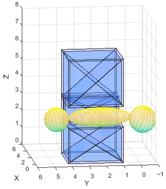
Figure 12. Compared spherical corridor with [15].

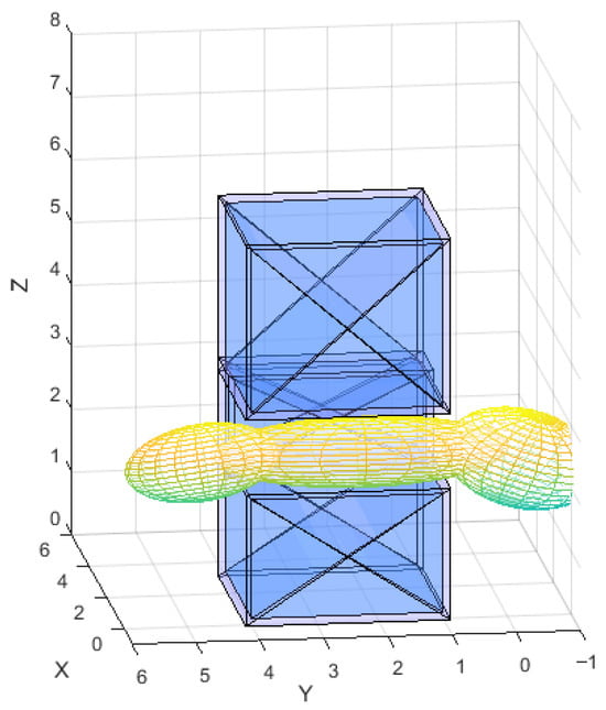
Figure 13. Proposed adaptive ellipsoidal corridor.

The proposed optimizer reduces the snap energy by 49% and the jerk energy by 31%, which directly translates into lower motor thrust-rate demands, smaller cable-swing amplitudes, and a 20% increase in actuator margin, while still allowing the corridor to be tightened ($\Delta w\downarrow 20\%$) and its spatial utilization to rise from 68% to 98%. Therefore, the improvement in the smoothness index not only represents numerical optimization but also enables simultaneous gains in compactness, safety, and trackability as reported in the paper.

As shown in Figure 12, the proposed adaptive corridor demonstrates significant performance improvements compared to the corridor presented in [15] (Figure 13). According to the summary in Table 3, although the adaptive corridor incurs a slight increase in generation time and memory usage, it achieves a remarkable 30-percentage-point gain in spatial utilization (increasing from 68% to 98%). This enhancement expands the feasible region for trajectory planning, enabling passage through areas previously inaccessible under symmetric hoisting configurations. Experimental results confirm that the proposed method substantially improves both spatial efficiency and corridor continuity but with less energy as shown in Table 4, thereby providing a more reliable safety margin for subsequent trajectory planning.

Table 3. Comparison of safe corridor performance.

Corridor Type	Gen. Time (s)	Memory Usage (MB)	Utilization (%)
Compared Corridor in [15]	0.018	0.188	68
Adaptive Corridor (Proposed)	0.023	0.242	98

Table 4. Comparison of path smoothness indices between the Compared SFC approach and the proposed method.

Method	Jerk Energy $\int \parallel {\mathit{p}}^{\left(3\right)}{\left(\mathit{t}\right)\parallel }^2\mathbf{d}\mathit{t}$	Snap Energy $\int \parallel {\mathit{p}}^{\left(4\right)}{\left(\mathit{t}\right)\parallel }^2\mathbf{d}\mathit{t}$
Compared SFC	5.0–6.8	23.7–31.4
Proposed Adaptive Corridor	3.5	15.9

6.3. Trajectory Planning and Tracking Results

The payload transportation system is designed to depart from the start point, navigate through the obstacle region depicted in Figure 14, and ultimately arrive at the target point. The design of closed-loop dynamic control is crucial for the actual tracking performance of the system. In our previous research, our team has conducted in-depth studies on trajectory tracking control for similar systems [22], with which the stable trajectory tracking can be effectively achieved while ensuring system dynamic stability, maintaining positive cable tension, and effectively suppressing load . The obstacles, represented by the blue rectangular prisms, have a height of 1 m, while the transportation system flies at an altitude of 1.2 m. With the help of results presented in Section 2.2, Section 3 and Section 4, as well as our control strategies [22], the system effectively avoids obstacles by dynamically adjusting both the inter-UAV angle and the flight trajectory as shown in Figure 14.

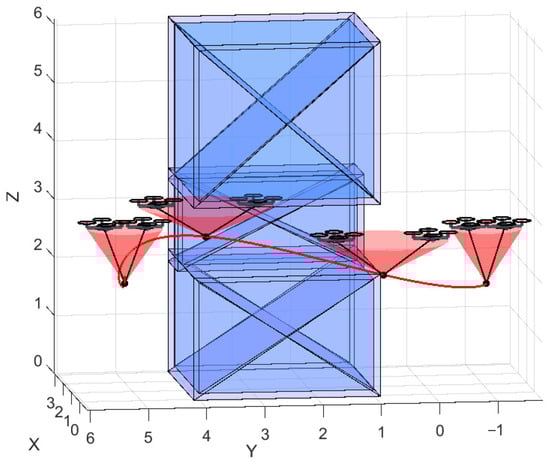
Figure 14. Navigating through the internal confined space within a large obstacle.

Based on the framework developed in this study, the symmetric UAV system was tested in a larger and more complex three-dimensional obstacle environment, as shown in Figure 15. To ensure safe passage through the complex environment, the system dynamically adjusts the inter-UAV angles and flight trajectories, as depicted in Figure 15. In the figure, the blue solid line represents the desired trajectory, while the black dashed line indicates the actual tracking trajectory. The tracking performance of the system is presented in Table 5, which shows the average error (AE) and maximum error (ME) percentages for different variables related to the load’s trajectory tracking. Specifically, $x_3$, $y_3$, and $z_3$ represent the average error percentages of the load’s three directional axes, while ${\theta }_1$ and ${\theta }_2$ indicate the maximum error percentages of the two swing angles. These error percentages are calculated by multiplying the ratio of the error value to the reference value (e.g., the total length of the trajectory) by 100%. As shown in the table, the system exhibits low error percentages, indicating high precision and reliability in trajectory tracking.

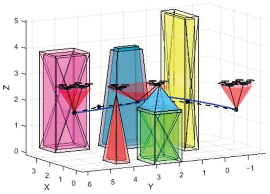
Figure 15. Three dimensional internal confined space within a large obstacle structure.

Table 5. Error Percentages for Different Metrics.

Metric	AE of ${\mathit{x}}_3$	AE of ${\mathit{y}}_3$	AE of ${\mathit{z}}_3$	ME of ${\mathit{\theta }}_1$	ME of ${\mathit{\theta }}_2$
Error Percentage	0.3851%	0.7532%	0.1101%	0.0204%	0.0203%

7. Discussion and Conclusions

This paper presents an integrated motion planning framework for symmetric UAV cooperative transportation. The core novelties lie in the RL-driven adaptive path planner, the formation-aware safe flight corridor, and their integration within a differential flatness-based optimization framework. This framework effectively addresses cooperative transportation challenges through unified path planning, corridor construction, and trajectory optimization.

The entire paper is developed under the symmetry and small-angle assumptions. If these assumptions are violated, the following failures occur:

• Differential-flatness breakdown
  The flat output $\mathit{\sigma }={[x_l,y_l,z_l,\varphi ]}^T$ is derived under the symmetry conditions ${\theta }_2={\theta }_1+\pi$ and $T_1\approx T_2$. If the two UAVs differ in position or tension (${\varphi }_1\ne {\varphi }_2$, ${\theta }_2-{\theta }_1\ne \pi$), the 4-D vector $\sigma$ can no longer algebraically parameterize the 9-D state vector q. Hence the dimensionality-reduction core of the minimum-snap optimizer vanishes; the trajectory must be planned in the full 9-D space, and the QP size and solution time explode.
• Constraint-linearization error blow-up
  The small-angle approximation ($\sin \theta \approx \theta$, $\cos \theta \approx 1$) turns Lagrangian dynamics into linear/quadratic constraints. For swing angles $>20°$–$30°$ the linearization error exceeds $10\%$, so the “smooth” optimal trajectory deviates significantly from real dynamics, producing negative cable tension (slack), thrust commands beyond motor saturation, and saturated tracking controllers that may become unstable.
• Safe-flight corridor misalignment
  The SFC treats the whole formation as one ellipsoid plus a sequence of convex polyhedra—valid only if symmetry fixes the relative UAV positions. Without symmetry, the UAV-payload triangle changes over time; the ellipsoid must be recomputed frame-by-frame or enveloped separately, leading to insufficient corridor volume (collision risk) or excessive corridor volume (space utilization collapses). collapses).

Future work will extend this approach to large-scale multi-UAV systems, dynamic environments, and real-world applications with perception uncertainties.

References

- Guo, L.; Li, Q. Path Planning of Mobile Robot Based on Improved RRT* Algorithm. Cogn. Syst. Res. 2024, 19, 1209–1217. [Google Scholar]
- Chen, Z.; Min, L.; Shao, X.; Zhao, Z. Obstacle Avoidance Path Planning of Bridge Crane Based on Improved RRT Algorithm. J. Syst. Simul. 2021, 33, 1832–1838. [Google Scholar]
- Alkomy, H.; Shan, J. Vibration reduction of a quadrotor with a cable-suspended payload using polynomial trajectories. Nonlinear Dyn. 2021, 104, 3713–3735. [Google Scholar] [CrossRef] [PubMed]
- Yu, G.; Chen, Y.; Chen, C.; Chen, X.; Mei, Y.; Liu, Y.; Xu, Y.; Zhang, W. Aggressive maneuvers for a quadrotor-slung-load system through fast trajectory generation and tracking. Auton. Robot. 2022, 46, 499–513. [Google Scholar] [CrossRef]
- Zhang, G.; Liu, X. UAV collision avoidance using mixed-integer second-order cone programming. J. Guid. Control. Dyn. 2022, 45, 1732–1738. [Google Scholar] [CrossRef]
- Li, X.; Zhang, J.; Han, J. Trajectory planning of load transportation with multi-quadrotors based on reinforcement learning algorithm. Aerosp. Sci. Technol. 2021, 116, 106887. [Google Scholar] [CrossRef]
- Estevez, J.; Gangoiti, U.; Lopez-Guede, J.M.; Graña, M. Reinforcement learning based trajectory planning for multi-UAV load transportation. IEEE Access 2024. [Google Scholar] [CrossRef]
- Campos-Macías, L.; Aldana-López, R.; de la Guardia, R.; Parra-Vilchis, J.I.; Gómez-Gutiérrez, D. Autonomous navigation of MAVs in unknown cluttered environments. J. Field Robot. 2021, 38, 307–326. [Google Scholar] [CrossRef]
- Duan, D.; Zu, R.; Yu, T.; Zhang, C.; Li, J. Differential flatness-based real-time trajectory planning for multihelicopter cooperative transportation in crowded environments. AIAA J. 2023, 61, 4079–4095. [Google Scholar] [CrossRef]
- Valentim, T.; Cunha, R.; Oliveira, P.; Cabecinhas, D.; Silvestre, C. Multi-vehicle cooperative control for load transportation. IFAC-PapersOnLine 2019, 52, 358–363. [Google Scholar] [CrossRef]
- Savin, S. An algorithm for generating convex obstacle-free regions based on stereographic projection. In Proceedings of the 2017 International Siberian Conference on Control and Communications (SIBCON), Astana, Kazakhstan, 29–30 June 2017; pp. 1–6. [Google Scholar]
- Zhong, X.; Wu, Y.; Wang, D.; Wang, Q.; Xu, C.; Gao, F. Generating large convex polytopes directly on point clouds. arXiv 2020, arXiv:2010.08744. [Google Scholar] [CrossRef]
- Werner, P.; Cohn, T.; Jiang, R.H.; Seyde, T.; Simchowitz, M.; Tedrake, R.; Rus, D. Faster algorithms for growing collision-free convex polytopes in robot configuration space. arXiv 2024, arXiv:2410.12649. [Google Scholar] [CrossRef]
- Ren, Y.; Zhu, F.; Liu, W.; Wang, Z.; Lin, Y.; Gao, F.; Zhang, F. Bubble planner: Planning high-speed smooth quadrotor trajectories using receding corridors. In Proceedings of the 2022 IEEE/RSJ International Conference on Intelligent Robots and Systems (IROS), Kyoto, Japan, 23–27 October 2022; pp. 6332–6339. [Google Scholar]
- Liu, S.; Watterson, M.; Mohta, K.; Sun, K.; Bhattacharya, S.; Taylor, C.J.; Kumar, V. Planning dynamically feasible trajectories for quadrotors using safe flight corridors in 3-D complex environments. IEEE Robot. Autom. Lett. 2017, 2, 1688–1695. [Google Scholar] [CrossRef]
- An, N.; Wang, Q.; Zhao, X.; Wang, Q. Differential Flatness and Formation Control of Unmanned Aerial Vehicle Swarm. J. Dyn. Control 2023, 21, 79–80. [Google Scholar]
- Zhang, H.; Huang, J. Research on Motion Planning of Tower Crane in Complex Environment. Control Eng. 2025, 32, 1833–1845. [Google Scholar]
- Lillicrap, T.P.; Hunt, J.J.; Pritzel, A.; Heess, N.; Erez, T.; Tassa, Y.; Silver, D.; Wierstra, D. Continuous control with deep reinforcement learning. arXiv 2015, arXiv:1509.02971. [Google Scholar]
- Karaman, S.; Frazzoli, E. Incremental Sampling-based Algorithms for Optimal Motion Planning. Int. J. Robot. Res. 2011, 30, 846–894. [Google Scholar] [CrossRef]
- Wang, H.F.; Zhang, Y.; Zhu, Y.K.; Chen, X.B. Path Planning Algorithm for Mobile Robot Based on Improved Bidirectional RRT*. J. Northeast. Univ. (Nat. Sci.) 2021, 42, 1065–1070. [Google Scholar]
- Shang, F.; Luo, C.; Li, W.; Liang, Y.; Xiao, W.; Chen, Q.; Zhou, X. Path Planning Research for Pitaya Picking Manipulator Based on APF-RRT*. J. Agric. Mech. Res. 2025, 47, 48–52. [Google Scholar]
- Huang, J.; Wang, Y.; Ni, L. Design of Cooperative Transportation and Anti-Sway Control for Dual UAVs. Comput. Integr. Manuf. Syst. 2025, 31, 4096–4104. [Google Scholar]
Disclaimer/Publisher’s Note: The statements, opinions and data contained in all publications are solely those of the individual author(s) and contributor(s) and not of MDPI and/or the editor(s). MDPI and/or the editor(s) disclaim responsibility for any injury to people or property resulting from any ideas, methods, instructions or products referred to in the content. |
© 2025 by the authors. Licensee MDPI, Basel, Switzerland. This article is an open access article distributed under the terms and conditions of the Creative Commons Attribution (CC BY) license (https://creativecommons.org/licenses/by/4.0/).