On the Solvability of Some Systems of Nonlinear Difference Equations

Abstract

The aim of this paper is to find formulas for the solutions of the nonlinear system of difference equations related to symmetry $P_{n+1}={\displaystyle \frac{T_n{T}_{n-2}}{-P_{n-3}-T_n}},T_{n+1}={\displaystyle \frac{P_n{P}_{n-2}}{\pm T_{n-3}\pm P_n}},$ where the initial conditions $P_{-3},P_{-2},P_{-1},P_0,T_{-3},T_{-2},T_{-1}$, and $T_0$ are arbitrary real numbers. Moreover, the theoretical results are verified through several numerical examples, which are simulated and graphically illustrated using mathematical programs.

1. Introduction

Nonlinear difference equations (NDEs) have recently gained significant attention from many researchers. Over the past decade, there has been a notable surge in interest in these types of equations. Their widespread applications across various fields not only in mathematics, but also in related disciplines such as biological sciences, engineering, ecology, discrete-time systems, economics, and physics, may have contributed to this growing fascination. Recent research has examined various aspects of nonlinear dynamics, including local and global behaviors, boundedness, topological classifications, and chaos analysis [1,2,3]. For instance, Khan et al. [4] investigated these dynamics within the framework of a discrete hepatitis C virus model. Similarly, Lei and Han [5] explored the dynamic behavior of a discrete predator–prey model incorporating fear and Allee effects through both theoretical analysis and numerical simulations.

We anticipate that as more intriguing and impactful results are discovered and shared through research, this area will continue to attract the curiosity of scholars in the coming years. The challenge of obtaining closed-form solutions for (NDEs) has become a central topic in this field of research. Many studies have attempted to address NDEs using various analytical and numerical techniques (see, for example, [6,7,8,9,10]), as these equations are often difficult to solve, especially when seeking exact solutions. To overcome this difficulty, several recent approaches have been proposed to transform complex nonlinear difference equations into linear forms, for which well-established solution techniques exist. For instance, a large class of NDEs has been successfully solved in closed form through linearization methods (see, [11,12,13,14]). Numerous researchers have also examined the dynamical behavior of systems of difference equations (SDEs). For example, Çinar analyzed the solutions of a specific SDE in [15], while Karakay et al. [16] demonstrated that certain subclasses of nonlinear two-dimensional SDEs can be solved in closed form. In addition, Halim et al. [17] provided a general formula for the solutions of two-dimensional SDEs, and El-Dessoky [18] explored the existence and periodic nature of such solutions. Khalil and Elsayed [19] studied systems of rational difference equations of various orders, derived explicit solution formulas for these systems, and analyzed their periodic behavior with different periods. Al-Juaid [20] investigated the structural properties of SDE solutions, whereas Alharbi [21] studied the dynamics of three-dimensional nonlinear SDEs, particularly those of fourth order. Alharthi [22] studied higher-order rational difference equation systems, derived their closed-form solutions, and investigated their periodic behavior. Further related studies on NDEs and SDEs can be found in [1,2,23].

Difference equations serve as suitable models for scenarios where population growth occurs in discrete, seasonal intervals with overlapping generations. In this context, researchers have examined the generalized Beverton–Holt stock recruitment model in [24]. Khaliq et al. [25] conducted a dynamical analysis of a discrete-time Lotka–Volterra model involving a system with two predators and one prey. Din and Elsayed [26] examined the boundedness, persistence, and local and global dynamics of a two-directional interacting invasive species model. In [27], the authors conducted a comprehensive study of the local dynamics of a discrete-time COVID-19 epidemic model, focusing on topological classifications, bifurcation analysis, and chaos control. See also [28,29,30].

In this paper, we focus on the following two-dimensional system, and we provide explicit solutions for several specific cases.

$$P_{n+1}={\displaystyle \frac{T_n{T}_{n-2}}{-P_{n-3}-T_n}},T_{n+1}={\displaystyle \frac{P_n{P}_{n-2}}{\pm T_{n-3}\pm P_n}},$$

(1)

where $n=0,1,2,\dots$ and the initial conditions $P_{n-i}$ and $T_{n-i}$ for $i\in \{-3,-2,-1,0\}$ are arbitrary nonzero real numbers.

The structure of the paper is as follows: Section 2 introduces the system under consideration and outlines the various cases derived from system (1), along with relevant theorems. Section 3 presents numerical simulations that support and validate the theoretical results. Section 4 offers a comprehensive discussion of the findings.

2. The Main Results

2.1. The First Case

In this section, we find the expressions of exact solution of the following system:

$$P_{n+1}={\displaystyle \frac{T_n{T}_{n-2}}{-P_{n-3}-T_n}},T_{n+1}={\displaystyle \frac{P_n{P}_{n-2}}{-T_{n-3}-P_n}}.$$

(2)

Theorem 1.

Suppose that $\{P_n,T_n\}$ are solutions of the SDEs (2). Then for $n=0,1,2,\dots$, the solutions of system (2) can be formed as follows:

$$P_{6n-3}={\displaystyle \frac{D^{2n}}{a^{n-1}{(-a-D)}^n}},T_{6n-3}={\displaystyle \frac{d^{2n}}{A^{n-1}{(-A-d)}^n}},$$

$$P_{6n-2}={\displaystyle \frac{d^{2n}b}{A^n{(-A-d)}^n}},T_{6n-2}={\displaystyle \frac{D^{2n}B}{a^n{(-a-D)}^n}},$$

$$P_{6n-1}={\displaystyle \frac{D^{2n}c}{a^n{(-a-D)}^n}},T_{6n-1}={\displaystyle \frac{d^{2n}C}{A^n{(-A-d)}^n}},$$

$$P_{6n}={\displaystyle \frac{d^{2n+1}}{A^n{(-A-d)}^n}},T_{6n}={\displaystyle \frac{D^{2n+1}}{a^n{(-a-D)}^n}},$$

$$P_{6n+1}={\displaystyle \frac{D^{2n+1}B}{a^n{(-a-D)}^{n+1}}},T_{6n+1}={\displaystyle \frac{d^{2n+1}b}{A^n{(-A-d)}^{n+1}}},$$

$$P_{6n+2}={\displaystyle \frac{d^{2n+1}C}{A^{n+1}{(-A-d)}^n}},T_{6n+2}={\displaystyle \frac{D^{2n+1}c}{a^{n+1}{(-a-D)}^n}},$$

where $P_{-3}=a$, $P_{-2}=b$, $P_{-1}=c$, $P_0=d$, $T_{-3}=A$, $T_{-2}=B$, $T_{-1}=C$, and $T_0=D$.

Proof. 

The results hold for $n=0$. Now for $n>0$, assume that the results are valid for $n-1$, as stated below

$$P_{6n-9}={\displaystyle \frac{D^{2n-2}}{a^{n-2}{(-a-D)}^{n-1}}},T_{6n-9}={\displaystyle \frac{d^{2n-2}}{A^{n-2}{(-A-d)}^{n-1}}},$$

$$P_{6n-8}={\displaystyle \frac{d^{2n-2}b}{A^{n-1}{(-A-d)}^{n-1}}},T_{6n-8}={\displaystyle \frac{D^{2n-2}B}{a^{n-1}{(-a-D)}^{n-1}}},$$

$$P_{6n-7}={\displaystyle \frac{D^{2n-2}c}{a^{n-1}{(-a-D)}^{n-1}}},T_{6n-7}={\displaystyle \frac{d^{2n-2}C}{A^{n-1}{(-A-d)}^{n-1}}},$$

$$P_{6n-6}={\displaystyle \frac{d^{2n-1}}{A^{n-1}{(-A-d)}^{n-1}}},T_{6n-6}={\displaystyle \frac{D^{2n-1}}{a^{n-1}{(-a-D)}^{n-1}}},$$

$$P_{6n-5}={\displaystyle \frac{D^{2n-1}B}{a^{n-1}{(-a-D)}^n}},T_{6n-5}={\displaystyle \frac{d^{2n-1}b}{A^{n-1}{(-A-d)}^n}},$$

$$P_{6n-4}={\displaystyle \frac{d^{2n-1}C}{A^n{(-A-d)}^{n-1}}},T_{6n-4}={\displaystyle \frac{D^{2n-1}c}{a^n{(-a-D)}^{n-1}}}.$$

Now, we prove the first relation.

Substituting $6n-3$ into system (2), we get

$$P_{6n-3}={\displaystyle \frac{T_{6n-4}{T}_{6n-6}}{-P_{6n-7}-T_{6n-4}}},$$

so

$$P_{6n-3}={\displaystyle \frac{\frac{D^{2n-1}c}{a^n{(-a-D)}^{n-1}}\frac{D^{2n-1}}{a^{n-1}{(-a-D)}^{n-1}}}{-\frac{D^{2n-2}c}{a^{n-1}{(-a-D)}^{n-1}}-\frac{D^{2n-1}c}{a^n{(-a-D)}^{n-1}}}};$$

then,

$$P_{6n-3}={\displaystyle \frac{D^{4n-2}c}{a^n{D}^{2n-1}c{(-a-D)}^{n-1}[-D^{-1}-a^{-1}]}}.$$

Therefore,

$$P_{6n-3}={\displaystyle \frac{D^{2n}}{a^{n-1}{(-a-D)}^n}}.$$

For equation $t_{6n-3}$, we can see from (2) that

$$T_{6n-3}={\displaystyle \frac{P_{6n-4}{P}_{6n-6}}{-T_{6n-7}-P_{6n-4}}};$$

that is,

$$T_{6n-3}={\displaystyle \frac{\frac{d^{2n-1}C}{A^n{(-A-d)}^{n-1}}\frac{d^{2n-1}}{A^{n-1}{(-A-d)}^{n-1}}}{-\frac{d^{2n-2}C}{A^{n-1}{(-A-d)}^{n-1}}-\frac{d^{2n-1}C}{A^n{(-A-d)}^{n-1}}}}.$$

Then,

$$T_{6n-3}={\displaystyle \frac{d^{4n-2}C}{A^n{d}^{2n-1}C{(-A-d)}^{n-1}[-d^{-1}-A^{-1}]}};$$

hence,

$$T_{6n-3}={\displaystyle \frac{d^{2n}}{A^{n-1}{(-A-d)}^n}}.$$

For the second formula, substituting $6n-2$ into (2), we get

$$P_{6n-2}={\displaystyle \frac{T_{6n-3}{T}_{6n-5}}{-P_{6n-6}-T_{6n-3}}};$$

then,

$$P_{6n-2}={\displaystyle \frac{\frac{d^{2n}}{A^{n-1}{(-A-d)}^n}\frac{d^{2n-1}b}{A^{n-1}{(-A-d)}^n}}{-\frac{d^{2n-1}}{A^{n-1}{(-A-d)}^{n-1}}-\frac{d^{2n}}{A^{n-1}{(-A-d)}^n}}},$$

so

$$P_{6n-2}={\displaystyle \frac{d^{2n-1}b{(-A-d)}^{-1}}{A^{n-1}{(-A-d)}^n\left(-d^{-1}-{(-A-d)}^{-1}\right)}}.$$

Thus,

$$P_{6n-2}={\displaystyle \frac{d^{2n}b}{A^n{(-A-d)}^n}}.$$

Now for equation $T_{6n-2}$, from (2) we get

$$T_{6n-2}={\displaystyle \frac{P_{6n-3}{P}_{6n-5}}{-T_{6n-6}-P_{6n-3}}};$$

that is,

$$T_{6n-2}={\displaystyle \frac{\frac{D^{2n}}{a^{n-1}{(-a-D)}^n}\frac{D^{2n-1}B}{a^{n-1}{(-a-D)}^n}}{-\frac{D^{2n-1}}{a^{n-1}{(-a-D)}^{n-1}}-\frac{D^{2n}}{a^{n-1}{(-a-D)}^n}}},$$

so

$$T_{6n-2}={\displaystyle \frac{D^{2n-1}B{(-a-D)}^{-1}}{a^{n-1}{(-a-D)}^n\left(-D^{-1}-{(-a-D)}^{-1}\right)}}.$$

Consequently,

$$T_{6n-2}={\displaystyle \frac{D^{2n}B}{a^n{(-a-D)}^n}},$$

Following the same approach, we can verify other forms. The proof is completed. □

2.2. The Second Case

This section is designed to discuss the form of solutions of the following system:

$$P_{n+1}={\displaystyle \frac{T_n{T}_{n-2}}{-P_{n-3}-T_n}},T_{n+1}={\displaystyle \frac{P_n{P}_{n-2}}{T_{n-3}-P_n}}.$$

(3)

Theorem 2.

Assume that $\{P_n,T_n\}$ are solutions of system (3). Then for $n\ge 0$, the solutions of system (3) can be formed as follows:

$$P_{12n-3}={\displaystyle \frac{{(-1)}^n{D}^{4n}}{a^{n-1}{(-a-2D)}^n{(-a-D)}^{2n}}},T_{12n-3}={\displaystyle \frac{{(-1)}^n{d}^{4n}}{A^{2n-1}{(A-d)}^n{(A+d)}^n}},$$

$$P_{12n-2}={\displaystyle \frac{{(-1)}^n{d}^{4n}b}{A^{2n}{(A-d)}^n{(A+d)}^n}},T_{12n-2}={\displaystyle \frac{{(-1)}^n{D}^{4n}B}{a^n{(-a-2D)}^n{(-a-D)}^{2n}}},$$

$$P_{12n-1}={\displaystyle \frac{{(-1)}^n{D}^{4n}c}{a^n{(-a-2D)}^n{(-a-D)}^{2n}}},T_{12n-1}={\displaystyle \frac{{(-1)}^n{d}^{4n}C}{A^{2n}{(A-d)}^n{(A+d)}^n}},$$

$$P_{12n}={\displaystyle \frac{{(-1)}^n{d}^{4n+1}}{A^{2n}{(A-d)}^n{(A+d)}^n}},T_{12n}={\displaystyle \frac{{(-1)}^n{D}^{4n+1}}{a^n{(-a-2D)}^n{(-a-D)}^{2n}}},$$

$$P_{12n+1}={\displaystyle \frac{{(-1)}^n{D}^{4n+1}B}{a^n{(-a-2D)}^n{(-a-D)}^{2n+1}}},T_{12n+1}={\displaystyle \frac{{(-1)}^n{d}^{4n+1}b}{A^{2n}{(A-d)}^{n+1}{(A+d)}^n}},$$

$$P_{12n+2}={\displaystyle \frac{{(-1)}^{n+1}{d}^{4n+1}C}{A^{2n+1}{(A-d)}^n{(A+d)}^n}},T_{12n+2}={\displaystyle \frac{{(-1)}^n{D}^{4n+1}c}{a^n{(-a-2D)}^{n+1}{(-a-D)}^{2n}}},$$

$$P_{12n+3}={\displaystyle \frac{{(-1)}^{n+1}{D}^{4n+2}}{a^n{(-a-2D)}^n{(-a-D)}^{2n+1}}},T_{12n+3}={\displaystyle \frac{{(-1)}^{n+1}{d}^{4n+2}}{A^{2n}{(A-d)}^n{(A+d)}^{n+1}}},$$

$$P_{12n+4}={\displaystyle \frac{{(-1)}^n{d}^{4n+2}b}{A^{2n+1}{(A-d)}^{n+1}{(A+d)}^n}},T_{12n+4}={\displaystyle \frac{{(-1)}^n{D}^{4n+2}B}{a^{n+1}{(-a-2D)}^n{(-a-D)}^{2n+1}}},$$

$$P_{12n+5}={\displaystyle \frac{{(-1)}^n{D}^{4n+2}c}{a^n{(-a-2D)}^{n+1}{(-a-D)}^{2n+1}}},T_{12n+5}={\displaystyle \frac{{(-1)}^{n+1}{d}^{4n+2}C}{A^{2n+1}{(A-d)}^{n+1}{(A+d)}^n}},$$

$$P_{12n+6}={\displaystyle \frac{{(-1)}^{n+1}{d}^{4n+3}}{A^{2n+1}{(A-d)}^n{(A+d)}^{n+1}}},T_{12n+6}={\displaystyle \frac{{(-1)}^{n+1}{D}^{4n+3}}{a^n{(-a-2D)}^{n+1}{(-a-D)}^{2n+1}}},$$

$$P_{12n+7}={\displaystyle \frac{{(-1)}^{n+1}{D}^{4n+3}B}{a^{n+1}{(-a-2D)}^n{(-a-D)}^{2n}}},T_{12n+7}={\displaystyle \frac{{(-1)}^{n+1}{d}^{4n+3}b}{A^{2n+1}{(A-d)}^{n+1}{(A+d)}^{n+1}}},$$

$$P_{12n+8}={\displaystyle \frac{{(-1)}^{n+1}{d}^{4n+3}C}{A^{2n+2}{(A-d)}^{n+1}{(A+d)}^n}},T_{12n+8}={\displaystyle \frac{{(-1)}^n{D}^{4n+3}c}{a^{n+1}{(-a-2D)}^{n+1}{(-a-D)}^{2n+1}}}.$$

Proof. 

It is evident that the results hold for the base case $n=0$. Now for $n>0$, assume that the results are valid for $n-1$ and are stated as follows:

$$P_{12n-15}={\displaystyle \frac{{(-1)}^{n-1}{D}^{4n-4}}{a^{n-2}{(-a-2D)}^{n-1}{(-a-D)}^{2n-2}}},T_{12n-15}={\displaystyle \frac{{(-1)}^{n-1}{d}^{4n-4}}{A^{2n-3}{(A-d)}^{n-1}{(A+d)}^{n-1}}},$$

$$P_{12n-14}={\displaystyle \frac{{(-1)}^{n-1}{d}^{4n-4}b}{A^{2n-2}{(A-d)}^{n-1}{(A+d)}^{n-1}}},T_{12n-14}={\displaystyle \frac{{(-1)}^{n-1}{D}^{4n-4}B}{a^{n-1}{(-a-2D)}^{n-1}{(-a-D)}^{2n-2}}},$$

$$P_{12n-13}={\displaystyle \frac{{(-1)}^{n-1}{D}^{4n-4}c}{a^{n-1}{(-a-2D)}^{n-1}{(-a-D)}^{2n-2}}},T_{12n-13}={\displaystyle \frac{{(-1)}^{n-1}{d}^{4n-4}C}{A^{2n-2}{(A-d)}^{n-1}{(A+d)}^{n-1}}},$$

$$P_{12n-12}={\displaystyle \frac{{(-1)}^{n-1}{d}^{4n-3}}{A^{2n-2}{(A-d)}^{n-1}{(A+d)}^{n-1}}},T_{12n-12}={\displaystyle \frac{{(-1)}^{n-1}{D}^{4n-3}}{a^{n-1}{(-a-2D)}^{n-1}{(-a-D)}^{2n-2}}},$$

$$P_{12n-11}={\displaystyle \frac{{(-1)}^{n-1}{D}^{4n-3}B}{a^{n-1}{(-a-2D)}^{n-1}{(-a-D)}^{2n-1}}},T_{12n-11}={\displaystyle \frac{{(-1)}^{n-1}{d}^{4n-3}b}{A^{2n-2}{(A-d)}^n{(A+d)}^{n-1}}},$$

$$P_{12n-10}={\displaystyle \frac{{(-1)}^n{d}^{4n-3}C}{A^{2n-1}{(-A+d)}^{n-1}{(A+d)}^{n-1}}},T_{12n-10}={\displaystyle \frac{{(-1)}^{n-1}{D}^{4n-3}c}{a^{n-1}{(-a-2D)}^n{(a-D)}^{2n-2}}},$$

$$P_{12n-9}={\displaystyle \frac{{(-1)}^n{D}^{4n-2}}{a^{n-1}{(-a-2D)}^{n-1}{(-a-D)}^{2n-1}}},T_{12n-9}={\displaystyle \frac{{(-1)}^n{d}^{4n-2}}{A^{2n-2}{(A-d)}^{n-1}{(A+d)}^n}},$$

$$P_{12n-8}={\displaystyle \frac{{(-1)}^{n-1}{d}^{4n-2}b}{A^{2n-1}{(A-d)}^n{(A+d)}^{n-1}}},T_{12n-8}={\displaystyle \frac{{(-1)}^{n-1}{D}^{4n-2}B}{a^n{(-a-2D)}^{n-1}{(-a-D)}^{2n-1}}},$$

$$P_{12n-7}={\displaystyle \frac{{(-1)}^{n-1}{D}^{4n-2}c}{a^{n-1}{(-a-2D)}^n{(-a-D)}^{2n-1}}},T_{12n-7}={\displaystyle \frac{{(-1)}^n{d}^{4n-2}C}{A^{2n-1}{(A-d)}^n{(A+d)}^{n-1}}},$$

$$P_{12n-6}={\displaystyle \frac{{(-1)}^n{d}^{4n-1}}{A^{2n-1}{(A-d)}^{n-1}{(A+d)}^n}},T_{12n-6}={\displaystyle \frac{{(-1)}^n{D}^{4n-1}}{a^{n-1}{(-a-2D)}^n{(-a-D)}^{2n-1}}},$$

$$P_{12n-5}={\displaystyle \frac{{(-1)}^n{D}^{4n-1}B}{a^n{(-a-2D)}^{n-1}{(-a-D)}^{2n-2}}},T_{12n-5}={\displaystyle \frac{{(-1)}^n{d}^{4n-1}b}{A^{2n-1}{(A-d)}^n{(A+d)}^n}},$$

$$P_{12n-4}={\displaystyle \frac{{(-1)}^n{d}^{4n-1}C}{A^{2n}{(A-d)}^n{(A+d)}^{n-1}}},T_{12n-4}={\displaystyle \frac{{(-1)}^{n-1}{D}^{4n-1}c}{a^n{(-a-2D)}^n{(-a-D)}^{2n-1}}}.$$

Now, we will demonstrate the first relation.

Substituting $12n-3$ into system (3), we get

$$P_{12n-3}={\displaystyle \frac{T_{12n-4}{T}_{12n-6}}{-P_{12n-7}-T_{12n-4}}};$$

then,

$$P_{12n-3}={\displaystyle \frac{\frac{{(-1)}^{n-1}{D}^{4n-1}c}{a^n{(-a-2D)}^n{(-a-D)}^{2n-1}}\frac{{(-1)}^n{D}^{4n-1}}{a^{n-1}{(-a-2D)}^n{(-a-D)}^{2n-1}}}{-\frac{{(-1)}^{n-1}{D}^{4n-2}c}{a^{n-1}{(-a-2D)}^n{(-a-D)}^{2n-1}}-\frac{{(-1)}^{n-1}{D}^{4n-1}c}{a^n{(-a-2D)}^n{(-a-D)}^{2n-1}}}},$$

so

$$P_{12n-3}={\displaystyle \frac{{(-1)}^n{D}^{4n-1}}{a^n{(-a-2D)}^n{(-a-D)}^{2n-1}[-D^{-1}-a^{-1}]}}.$$

Therefore,

$$P_{12n-3}={\displaystyle \frac{{(-1)}^n{D}^{4n}}{a^{n-1}{(-a-2D)}^n{(-a-D)}^{2n}}}.$$

For equation $T_{12n-3}$, we get from (3)

$$T_{12n-3}={\displaystyle \frac{P_{12n-4}{P}_{12n-6}}{T_{12n-7}-P_{12n-4}}};$$

that is,

$$T_{12n-3}={\displaystyle \frac{\frac{{(-1)}^n{d}^{4n-1}C}{A^{2n}{(A-d)}^n{(A+d)}^{n-1}}\frac{{(-1)}^n{d}^{4n-1}}{A^{2n-1}{(A-d)}^{n-1}{(A+d)}^n}}{\frac{{(-1)}^n{d}^{4n-2}C}{A^{2n-1}{(A-d)}^n{(A+d)}^{n-1}}-\frac{{(-1)}^n{d}^{4n-1}C}{A^{2n}{(A-d)}^n{(A+d)}^{n-1}}}}.$$

Then,

$$T_{12n-3}={\displaystyle \frac{{(-1)}^n{d}^{4n-1}}{A^{2n}{(A-d)}^{n-1}{(A+d)}^n[d^{-1}-A^{-1}]}}.$$

Consequently,

$$T_{12n-3}={\displaystyle \frac{{(-1)}^n{d}^{4n}}{A^{2n-1}{(A-d)}^n{(A+d)}^n}}.$$

In a similar way, we can prove the remaining relations. The proof is completed. □

2.3. The Third Case

In this part, we show the formula of solutions for the following nonlinear system:

$$P_{n+1}={\displaystyle \frac{T_n{T}_{n-2}}{-P_{n-3}-T_n}},T_{n+1}={\displaystyle \frac{P_n{P}_{n-2}}{T_{n-3}+P_n}}.$$

(4)

Theorem 3.

Suppose that $\{P_n,T_n\}$ are solutions of the system (4). Then for $n=0,1,2,3,\dots$, the solutions of system (4) can be formed as follows:

$$P_{12n-3}={\displaystyle \frac{D^{4n}}{a^{2n-1}{(-a+D)}^n{(-a-D)}^n}},T_{12n-3}={\displaystyle \frac{d^{4n}}{A^{n-1}{(A+d)}^{2n}{(A+2d)}^n}},$$

$$P_{12n-2}={\displaystyle \frac{d^{4n}b}{A^n{(A+d)}^{2n}{(A+2d)}^n}},T_{12n-2}={\displaystyle \frac{D^{4n}B}{a^{2n}{(-a+D)}^n{(-a-D)}^n}},$$

$$P_{12n-1}={\displaystyle \frac{D^{4n}c}{a^{2n}{(-a+D)}^n{(-a-D)}^n}},T_{12n-1}={\displaystyle \frac{d^{4n}C}{A^n{(A+d)}^{2n}{(A+2d)}^n}},$$

$$P_{12n}={\displaystyle \frac{d^{4n+1}}{A^n{(A+d)}^{2n}{(A+2d)}^n}},T_{12n}={\displaystyle \frac{D^{4n+1}}{a^{2n}{(-a+D)}^n{(-a-D)}^n}},$$

$$P_{12n+1}={\displaystyle \frac{D^{4n+1}B}{a^{2n}{(-a+D)}^n{(-a-D)}^{n+1}}},T_{12n+1}={\displaystyle \frac{-d^{4n+1}b}{A^n{(A+d)}^{2n+1}{(A+2d)}^n}},$$

$$P_{12n+2}={\displaystyle \frac{-d^{4n+1}C}{A^n{(A+d)}^{2n}{(A+2d)}^{n+1}}},T_{12n+2}={\displaystyle \frac{-D^{4n+1}c}{a^{2n+1}{(-a+D)}^n{(-a-D)}^n}},$$

$$P_{12n+3}={\displaystyle \frac{-D^{4n+2}}{a^{2n}{(-a+D)}^{n+1}{(-a-D)}^n}},T_{12n+3}={\displaystyle \frac{d^{4n+2}}{A^n{(A+d)}^{2n+1}{(A+2d)}^n}},$$

$$P_{12n+4}={\displaystyle \frac{-d^{4n+2}b}{A^{n+1}{(A+d)}^{2n+1}{(A+2d)}^n}},T_{12n+4}={\displaystyle \frac{D^{4n+2}B}{a^{2n+1}{(-a+D)}^n{(-a-D)}^{n+1}}},$$

$$P_{12n+5}={\displaystyle \frac{-D^{4n+2}c}{a^{2n+1}{(-a+D)}^n{(-a-D)}^{n+1}}},T_{12n+5}={\displaystyle \frac{d^{4n+2}C}{A^n{(A+d)}^{2n+1}{(A+2d)}^{n+1}}},$$

$$P_{12n+6}={\displaystyle \frac{d^{4n+3}}{A^n{(A+d)}^{2n+1}{(A+2d)}^{n+1}}},T_{12n+6}={\displaystyle \frac{D^{4n+3}}{a^{2n+1}{(-a+D)}^{n+1}{(-a-D)}^n}},$$

$$P_{12n+7}={\displaystyle \frac{-D^{4n+3}B}{a^{2n+1}{(-a+D)}^{n+1}{(-a-D)}^{n+1}}},T_{12n+7}={\displaystyle \frac{-d^{4n+3}b}{A^{n+1}{(A+d)}^{2n+2}{(A+2d)}^n}},$$

$$P_{12n+8}={\displaystyle \frac{d^{4n+3}C}{A^{n+1}{(A+d)}^{2n+1}{(A+2d)}^{n+1}}},T_{12n+8}={\displaystyle \frac{-D^{4n+3}c}{a^{2n+2}{(-a+D)}^n{(-a-D)}^{n+1}}}.$$

Proof. 

See Appendix A □

2.4. The Fourth Case

The formula of solutions is explored for the nonlinear system of difference Equation (5) in this section.

$$P_{n+1}={\displaystyle \frac{T_n{T}_{n-2}}{-P_{n-3}-T_n}},T_{n+1}={\displaystyle \frac{P_n{P}_{n-2}}{-T_{n-3}+P_n}}.$$

(5)

Theorem 4.

Let $\{P_n,T_n\}$ be solutions of system (5). Then for $n=0,1,2,3,\dots$, the solutions of system (5) can be formed as follows:

$$\begin{array}{cc}\hfill P_{6n-3}& ={\displaystyle \frac{a{D}^{2n}}{{\prod }_{i=0}^{n-1}(-a-\left(6i\right)D)(-a-(6i+3)D)}},\hfill \\ \hfill T_{6n-3}& ={\displaystyle \frac{A{d}^{2n}}{{\prod }_{i=0}^{n-1}(-A+\left(6i\right)d)(-A+(6i+3)d)}},\hfill \end{array}$$

$$\begin{array}{cc}\hfill P_{6n-2}& ={\displaystyle \frac{-d^{2n}b}{{\prod }_{i=0}^{n-1}(-A+(6i+1)d)(-A+(6i+4)d)}},\hfill \\ \hfill T_{6n-2}& ={\displaystyle \frac{-D^{2n}B}{{\prod }_{i=0}^{n-1}(-a-(6i+1)D)(-a-(6i+4)D)}},\hfill \end{array}$$

$$\begin{array}{c}\hfill P_{6n-1}={\displaystyle \frac{-D^{2n}c}{{\prod }_{i=0}^{n-1}(-a-(6i+2)D)(-a-(6i+5)D)}},\\ \hfill T_{6n-1}={\displaystyle \frac{-d^{2n}C}{{\prod }_{i=0}^{n-1}(-A+(6i+2)d)(-A+(6i+5)d)}},\end{array}$$

$$\begin{array}{c}\hfill P_{6n}={\displaystyle \frac{-d^{2n+1}}{{\prod }_{i=0}^{n-1}(-A+(6i+3)d)(-A+(6i+6)d)}},\\ \hfill T_{6n}={\displaystyle \frac{-D^{2n+1}}{{\prod }_{i=0}^{n-1}(-a-(6i+3)D)(-a-(6i+6)D)}},\end{array}$$

$$\begin{array}{c}\hfill P_{6n+1}={\displaystyle \frac{D^{2n+1}B}{(-a-D){\prod }_{i=0}^{n-1}(-a-(6i+4)D)(-a-(6i+7)D)}},\\ \hfill T_{6n+1}={\displaystyle \frac{d^{2n+1}b}{(-A+d){\prod }_{i=0}^{n-1}(-A+(6i+4)d)(-A+(6i+7)d)}},\end{array}$$

$$\begin{array}{c}\hfill P_{6n+2}={\displaystyle \frac{-d^{2n+1}C}{(-A+2d){\prod }_{i=0}^{n-1}(-A+(6i+5)d)(-A+(6i+8)d)}},\\ \hfill T_{6n+2}={\displaystyle \frac{-D^{2n+1}c}{(-a-2D){\prod }_{i=0}^{n-1}(-a-(6i+5)D)(-a-(6i+8)D)}}.\end{array}$$

Proof. 

The results are true for $n=0$. Now for $n>0$, assume the results hold for $n-1$ and they are given as follows:

$$\begin{array}{c}\hfill P_{6n-9}={\displaystyle \frac{a{D}^{2n-2}}{{\prod }_{i=0}^{n-2}(-a-\left(6i\right)D)(-a-(6i+3)D)}},\\ \hfill T_{6n-9}={\displaystyle \frac{A{d}^{2n-2}}{{\prod }_{i=0}^{n-2}(-A+\left(6i\right)d)(-A+(6i+3)d)}},\end{array}$$

$$\begin{array}{c}\hfill P_{6n-8}={\displaystyle \frac{-d^{2n-2}b}{{\prod }_{i=0}^{n-2}(-A+(6i+1)d)(-A+(6i+4)d)}},\\ \hfill T_{6n-8}={\displaystyle \frac{-D^{2n-2}B}{{\prod }_{i=0}^{n-2}(-a-(6i+1)D)(-a-(6i+4)D)}},\end{array}$$

$$\begin{array}{c}\hfill P_{6n-7}={\displaystyle \frac{-D^{2n-2}c}{{\prod }_{i=0}^{n-2}(-a-(6i+2)D)(-a-(6i+5)D)}},\\ \hfill T_{6n-7}={\displaystyle \frac{-d^{2n-2}C}{{\prod }_{i=0}^{n-2}(-A+(6i+2)d)(-A+(6i+5)d)}},\end{array}$$

$$\begin{array}{c}\hfill P_{6n-6}={\displaystyle \frac{-d^{2n-1}}{{\prod }_{i=0}^{n-2}(-A+(6i+3)d)(-A+(6i+6)d)}},\\ \hfill T_{6n-6}={\displaystyle \frac{-D^{2n-1}}{{\prod }_{i=0}^{n-2}(-a-(6i+3)D)(-a-(6i+6)D)}},\end{array}$$

$$\begin{array}{c}\hfill P_{6n-5}={\displaystyle \frac{D^{2n-1}B}{(-a-D){\prod }_{i=0}^{n-2}(-a-(6i+4)D)(-a-(6i+7)D)}},\\ \hfill T_{6n-5}={\displaystyle \frac{d^{2n-1}b}{(-A+d){\prod }_{i=0}^{n-2}(-A+(6i+4)d)(-A+(6i+7)d)}},\end{array}$$

$$\begin{array}{c}\hfill P_{6n-4}={\displaystyle \frac{-d^{2n-1}C}{(-A+2d){\prod }_{i=0}^{n-2}(-A+(6i+5)d)(-A+(6i+8)d)}},\\ \hfill T_{6n-4}={\displaystyle \frac{-D^{2n-1}c}{(-a-2D){\prod }_{i=0}^{n-2}(-a-(6i+5)D)(-a-(6i+8)D)}}.\end{array}$$

We will prove the first formula.

Substituting $6n-3$ into the SDEs (5), we get

$$\begin{array}{cc}\hfill P_{6n-3}& ={\displaystyle \frac{T_{6n-4}{T}_{6n-6}}{-P_{6n-7}-T_{6n-4}}},\hfill \\ \\ \hfill P_{6n-3}& ={\displaystyle \frac{\frac{-D^{2n-1}c}{(-a-2D){\prod }_{i=0}^{n-2}(-a-(6i+5)D)(-a-(6i+8)D)}\frac{-D^{2n-1}}{{\prod }_{i=0}^{n-2}(-a-(6i+3)D)(-a-(6i+6)D)}}{-\frac{-D^{2n-2}c}{{\prod }_{i=0}^{n-2}(-a-(6i+2)D)(-a-(6i+5)D)}-\frac{-D^{2n-1}c}{(-a-2D){\prod }_{i=0}^{n-2}(-a-(6i+5)D)(-a-(6i+8)D)}}}.\hfill \\ \end{array}$$

Accordingly,

$$\begin{array}{cc}\hfill P_{6n-3}& ={\displaystyle \frac{D^{2n}}{{\prod }_{i=0}^{n-2}(-a-(6i+3)D)(-a-(6i+6)D)\left((-a-(6n-4\left)D\right)-D\right)}}.\hfill \end{array}$$

Hence,

$$\begin{array}{cc}\hfill P_{6n-3}& ={\displaystyle \frac{a{D}^{2n}}{{\prod }_{i=0}^{n-1}(-a-\left(6i\right)D)(-a-(6i+3)D)}},\hfill \end{array}$$

For equation $T_{12n-3}$, we get from (5)

$$\begin{array}{cc}\hfill T_{6n-3}& ={\displaystyle \frac{P_{6n-4}{P}_{6n-6}}{-T_{6n-7}+P_{6n-4}}},\hfill \\ \\ \hfill T_{6n-3}& ={\displaystyle \frac{\frac{-d^{2n-1}C}{(A-2d){\prod }_{i=0}^{n-2}(-A+(6i+5)d)(-A+(6i+8)d)}\frac{-d^{2n-1}}{{\prod }_{i=0}^{n-2}(-A+(6i+3)d)(-A+(6i+6)d)}}{-\frac{-d^{2n-2}C}{{\prod }_{i=0}^{n-2}(-A+(6i+2)d)(-A+(6i+5)d)}+\frac{-d^{2n-1}C}{(-A+2d){\prod }_{i=0}^{n-2}(-A+(6i+5)d)(-A+(6i+8)d)}}},\hfill \end{array}$$

$$T_{6n-3}={\displaystyle \frac{d^{2n}}{{\prod }_{i=0}^{n-2}(-A+(6i+3)d)(-A+(6i+6)d)\left((-A+(6n-4)d-d)\right)}}.$$

Consequently,

$$T_{6n-3}={\displaystyle \frac{A{d}^{2n}}{{\prod }_{i=0}^{n-1}(-A+\left(6i\right)d)(-A+(6i+3)d)}}.$$

Likewise, we can prove other formulas. The proof is completed. □

3. Numerical Examples

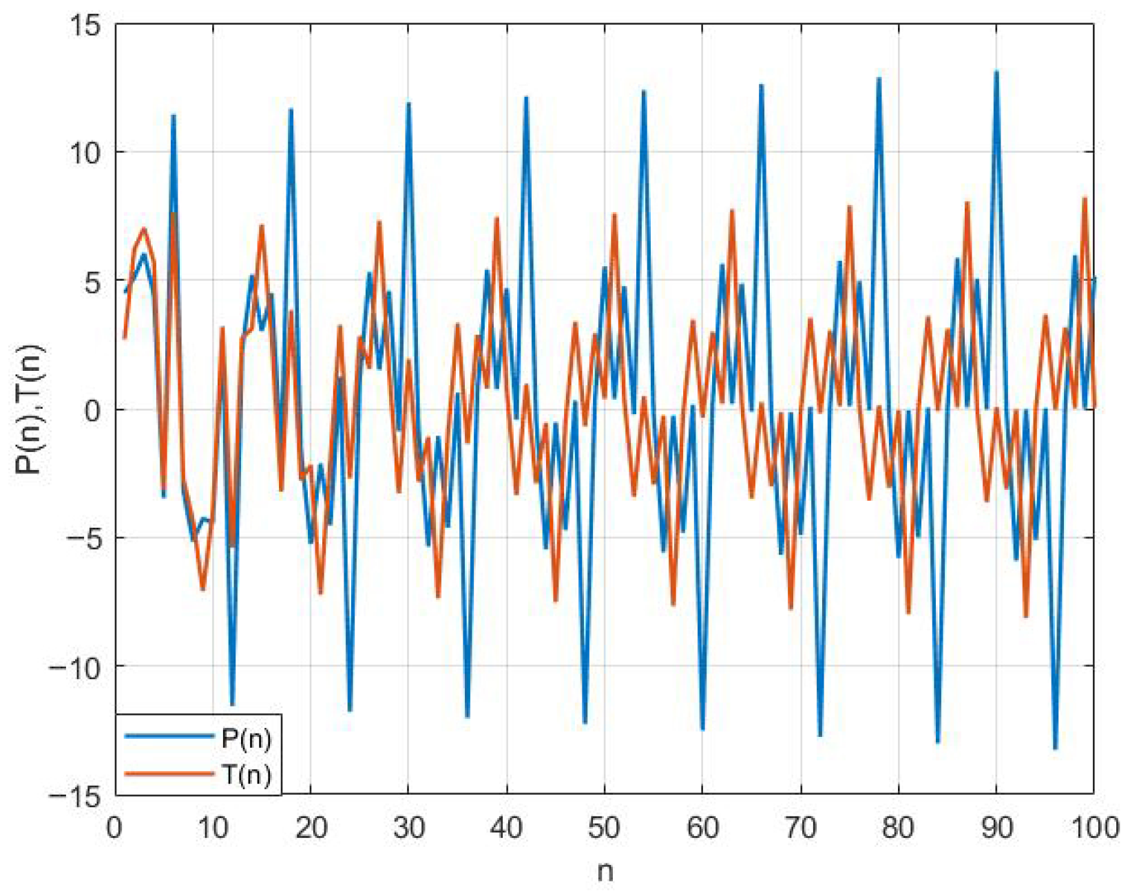
In this section, we provide several interesting numerical examples that validate our earlier theoretical findings and reinforce the correctness of our proofs. Additionally, these examples demonstrate the behavior of various solutions to the nonlinear systems explored in the previous sections. All of the plots (Figure 1, Figure 2, Figure 3 and Figure 4) in this section were generated using MATLAB (R2024b).

Example 1.

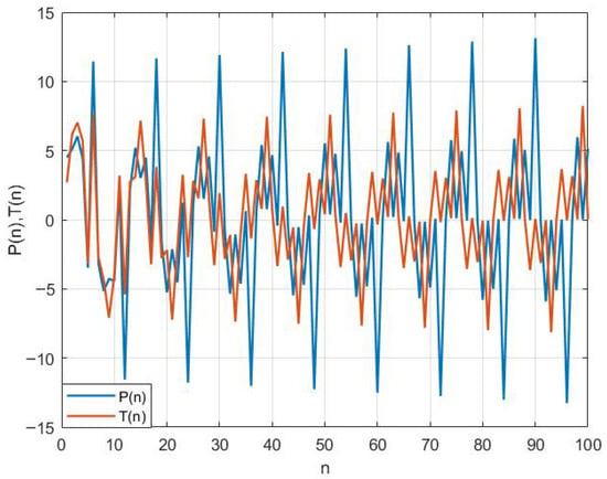
Figure 1 shows the behavior of the first system (2) under the random values $P_{-3}=4.5$, $P_{-2}=5.1$, $P_{-1}=6.03$, $P_0=4.4$, $T_{-3}=2.7$, $T_{-2}=6.2$, $T_{-1}=7.02$, and $T_0=5.7$.

Figure 1. Representation of behavior of System (2) when $P_{-3}=4.5$, $P_{-2}=5.1$, $P_{-1}=6.03$, $P_0=4.4$, $T_{-3}=2.7$, $T_{-2}=6.2$, $T_{-1}=7.02$, and $T_0=5.7$.

Example 2.

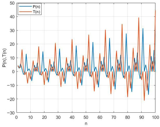
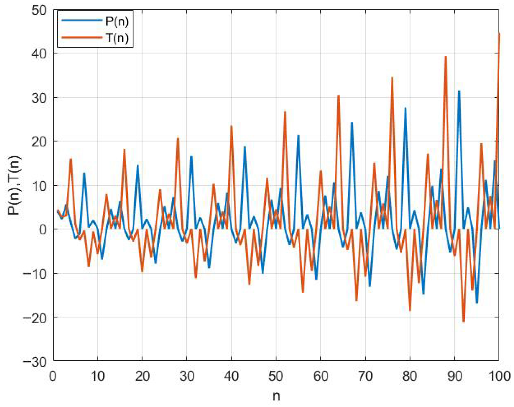
In Figure 2, we present the dynamics of the system (3) with the initial conditions $P_{-3}=4.01$, $P_{-2}=2.3$, $P_{-1}=5.6$, $P_0=1.5$, $T_{-3}=4.41$, $T_{-2}=2.07$, $T_{-1}=3.1$, and $T_0=16.03$.

Figure 2. Behavior of System (3) with $P_{-3}=4.01$, $P_{-2}=2.3$, $P_{-1}=5.6$, $P_0=1.5$, $T_{-3}=4.41$, $T_{-2}=2.07$, $T_{-1}=3.1$, and $T_0=16.03$.

Example 3.

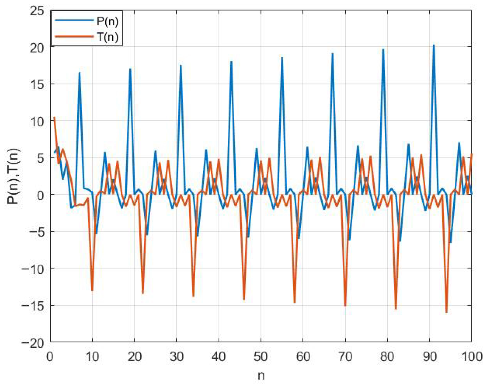
This example illustrates the behavior of the solutions of system (4), which is simulated in Figure 3 using the initial conditions $P_{-3}=5.6$, $P_{-2}=6.5$, $P_{-1}=2$, $P_0=4.5$, $T_{-3}=10.5$, $T_{-2}=4.10$, $T_{-1}=6.2$, and $T_0=4.42$.

Figure 3. Expression of the solution of System (4) when $P_{-3}=5.6$, $P_{-2}=6.5$, $P_{-1}=2$, $P_0=4.5$, $T_{-3}=10.5$, $T_{-2}=4.10$, $T_{-1}=6.2$, and $T_0=4.42$.

Example 4.

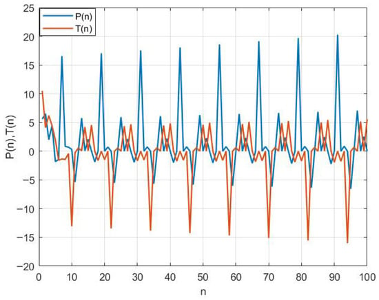
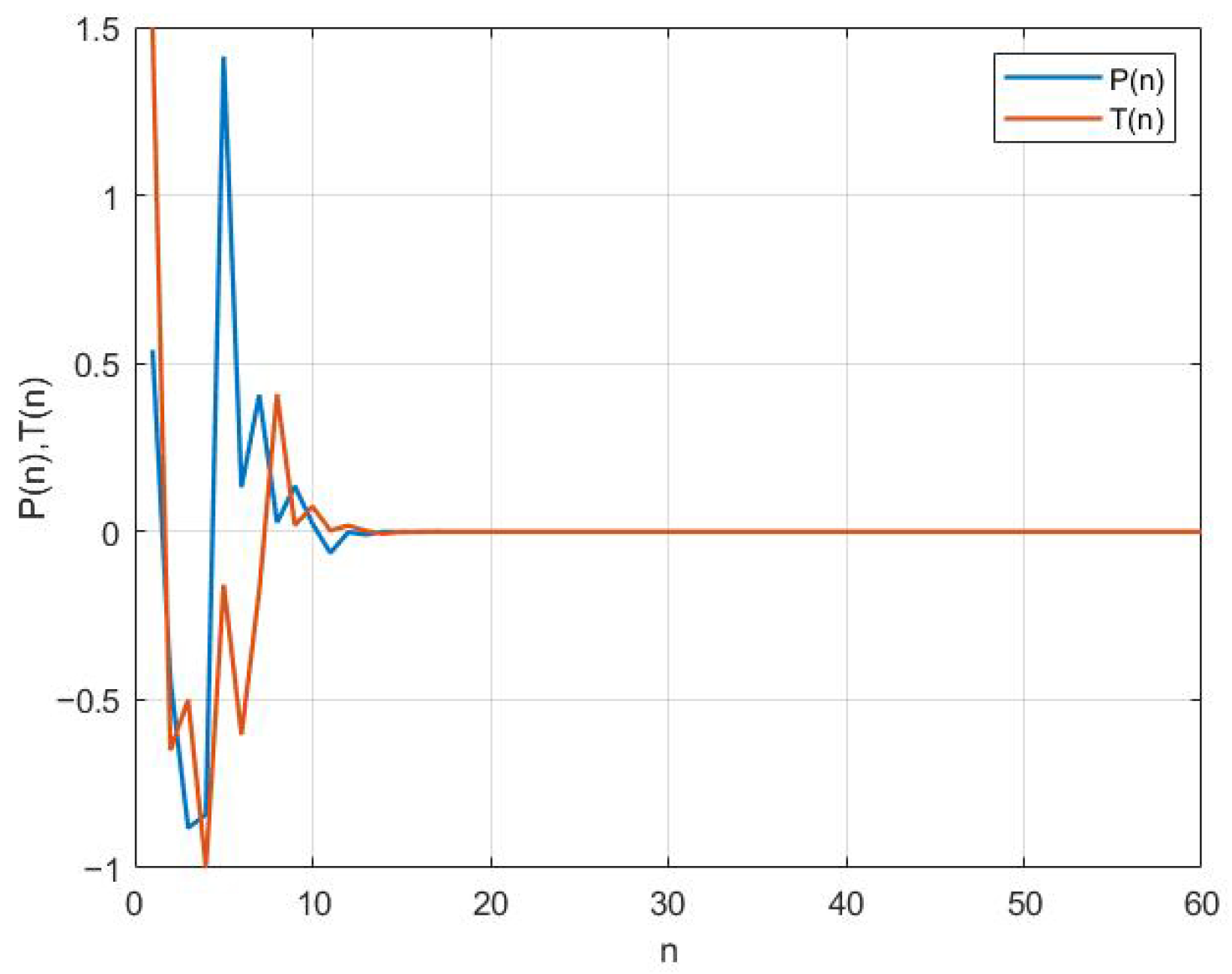
Figure 4 shows that the solution of the fourth system (5) approaches zero as n goes to ∞ with the initial values $P_{-3}=0.54$, $P_{-2}=-0.44$, $P_{-1}=-0.881$, $P_0=-0.841$, $T_{-3}=1.5$, $T_{-2}=-0.65$, $T_{-1}=-0.50$, and $T_0=-1$.

Figure 4. Plot of solutions of System (5) with $P_{-3}=0.54$, $P_{-2}=-0.44$, $P_{-1}=-0.881$, $P_0=-0.841$, $T_{-3}=1.5$, $T_{-2}=-0.65$, $T_{-1}=-0.50$, and $T_0=-1$.

4. Conclusions

This paper examines the dynamics of nonlinear systems of difference equations, with particular emphasis on fourth-order cases. Our primary goal was to provide analytical solutions for various systems by employing an iterative approach to obtain explicit solution formulas for systems of Equation (1) characterized by recursive relationships. We first found the general solution for system (2) and then obtained the solution formulas for systems (3)–(5). To validate the theoretical findings, numerical simulations were performed and visualized using mathematical software. These simulations demonstrate the accuracy and applicability of the solutions. Overall, the results make a meaningful contribution to the study of nonlinear systems and have significant implications for their applications across various scientific disciplines.

References

1. Althagafi, H. Dynamics of difference systems: A mathematical study with applications to neural systems. AIMS Math. 2025, 10, 2869–2890. [Google Scholar] [CrossRef]
2. Alharbi, T.D.; Hasan, M.R. On the Dynamics of Some Higher-Order Nonlinear Difference Equations. Mathematics 2024, 12, 3810. [Google Scholar] [CrossRef]
3. Ahlbrandt, C.D.; Peterson, A.C. Discrete Hamiltonian Systems: Difference Equations, Continued Fractions, and Riccati Equations; Kluwer Academic Publishers: Dordrecht, The Netherlands, 1996. [Google Scholar]
4. Khan, A.Q.; Ayesha, Y.; Alsaadi, A. Discrete Hepatitis C virus model with local dynamics, chaos and bifurcations. AIMS Math. 2024, 9, 28643–28670. [Google Scholar] [CrossRef]
5. Lei, C.; Han, X. Codimension-two bifurcation analysis of a discrete predator–prey system with fear effect and Allee effect. Nonlinear Anal. Model. Control. 2025, 30, 386–404. [Google Scholar] [CrossRef]
6. Ogul, B.; Simsek, D. On the recursive sequence, Dynamics of Continuous. Discret. Impuls. Syst. Ser. B Appl. Algorithms 2022, 29, 423–435. [Google Scholar]
7. Folly-Gbetoula, M.; Gocen, M.; Guneysu, M. General form of the solutions of some difference equations via Lie symmetry analysis. J. Anal. Appl. 2022, 20, 105–122. [Google Scholar]
8. Elsayed, E.M.; AL-Juaid, J.G. The form of solutions and periodic nature for some system of difference equations. Fundam. J. Math. Appl. 2023, 6, 24–34. [Google Scholar] [CrossRef]
9. Alharbi, T.D.; Elsayed, E.M. The solution expression and the periodicity solution of some nonlinear discrete systems. Pan-Am. J. Math. 2023, 2, 3. [Google Scholar] [CrossRef] [PubMed]
10. Kara, M. Solvability of a three-dimensional system of nonlinear difference equations. Math. Sci. Appl. E-Notes 2022, 10, 1–15. [Google Scholar] [CrossRef]
11. Das, S.E.; Bayram, M. On a system of rational difference equations. World Appl. Sci. J. 2010, 10, 1306–1312. [Google Scholar]
12. Dilip, D.S.; Mathew, S.M. Dynamics of a second order nonlinear difference system with exponents. J. Egypt. Math. Soc. 2021, 29, 1–10. [Google Scholar] [CrossRef]
13. Elabbasy, E.M.; Eleissawy, S.M. Asymptotic behavior of two dimensional rational system of difference equations. Dyn. Contin. Impuls. Syst. Ser. B Appl. Algorithms 2013, 20, 221–235. [Google Scholar]
14. Elabbasy, E.M.; El-Metwally, H.; Elsayed, E.M. Global behavior of the solutions of difference equation. Adv. Differ. Equ. 2011, 28, 1–16. [Google Scholar] [CrossRef]
15. Cinar, C.; Yalcinkaya, I.; Karatas, R. On the positive solutions of the difference equation system xn+1 = m y n , yn+1 = p y n x n 1 y n 1 . J. Inst. Math. Comp. Sci. 2005, 18, 135–136. [Google Scholar]
16. Karakaya, D.; Yasin, Y.; Kara, M. On A solvable system Of difference equations of sixth-order. Miskolc Math. Notes 2023, 24, 1405–1426. [Google Scholar] [CrossRef]
17. Halim, Y.; Khelifa, A.; Berkal, M. Representation of solutions of a two-dimensional system of difference equations. Miskolc Math. Notes 2020, 21, 203–218. [Google Scholar] [CrossRef]
18. El-Dessoky, M.M.; Elsayed, E.M.; Alghamdi, M. Solutions and periodicity for some systems of fourth order rational difference equations. J. Comput. Anal. Appl. 2025, 18, 179–194. [Google Scholar]
19. Al-Basyouni, K.S.; Elsayed, E.M. On Some Solvable Systems of Some Rational Difference Equations of Third Order. Mathematics 2023, 11, 1047. [Google Scholar] [CrossRef]
20. Elsayed, E.M.; AL-Juaid, J.G.; Malaikah, H. On the solutions of systems of rational difference equations. J. Progress. Res. Math. 2022, 19, 49–59. [Google Scholar] [CrossRef]
21. Alharbi, T.D.; AL-Juaid, J.G. On the dynamics of some three-dimensional systems of difference equations. Axioms 2025, 14, 371. [Google Scholar] [CrossRef]
22. Alharthi, M.T. On the solutions of some systems of rational difference equations. AIMS Math. 2024, 9, 30320–30347. [Google Scholar] [CrossRef]
23. Almatra, M.B.; Elsayed, E.M. Solutions and formulae for some systems of difference equations. MathLAB J. 2018, 1, 356–369. [Google Scholar]
24. Beverton, R.J.; Holt, S.J. On the Dynamics of Exploited Fish Populations; Fish Invest: London, UK, 1957; p. 19. [Google Scholar]
25. Khaliq, A.; Ibrahim, T.F.; Alotaibi, A.M.; Shoaib, M.; El-Moneam, M. Dynamical analysis of discrete-time two-predators one-Prey Lotka–Volterra model. Mathematics 2022, 10, 4015. [Google Scholar] [CrossRef]
26. Din, Q.; Elsayed, E.M. Stability analysis of a discrete ecological. Model. Comput. Ecol. Softw. 2014, 4, 89–103. [Google Scholar]
27. Khan, A.Q.; Tasneem, M.; Younis, B.; Ibrahim, T.F. Dynamical analysis of a discrete-time COVID-19 epidemic model. Math. Meth. Appl. Sci. 2022, 46, 4789–4814. [Google Scholar] [CrossRef]
28. Al-Khedhairi, A.; Elsadany, A.A.; Elsonbaty, A. On the dynamics of a discrete fractional-order cournot–bertrand competition duopoly game. Math. Probl. Eng. 2022, 2022, 8249215. [Google Scholar] [CrossRef]
29. Ibrahim, T.F. Asymptotic behavior of a difference equation model in exponential form. Math. Methods Appl. Sci. 2022, 45, 10736–10748. [Google Scholar] [CrossRef]
30. Khaliq, A.; Mustafa, I.; Ibrahim, T.F.; Osman, W.M.; Al-Sinan, B.R.; Dawood, A.A.; Juma, M.Y. Stability and bifurcation analysis of fifth-order nonlinear fractional difference equation. Fractal Fract. 2023, 7, 113. [Google Scholar] [CrossRef]
Disclaimer/Publisher’s Note: The statements, opinions and data contained in all publications are solely those of the individual author(s) and contributor(s) and not of MDPI and/or the editor(s). MDPI and/or the editor(s) disclaim responsibility for any injury to people or property resulting from any ideas, methods, instructions or products referred to in the content.
Article Metrics
Citations
Article Access Statistics
Article metric data becomes available approximately 24 hours after publication online.