Asymptotic Analysis of Generalized Logistic Affiliation Network Models with Node Attributes

Abstract

Affiliation networks, with their bipartite structure and non-binary features, pose unique challenges due to their complex relationships and diverse node attributes. These challenges differ from those in symmetric one-mode networks. To address them, we propose a generalized logistic affiliation network model. Despite the structural asymmetry, the model incorporates node attributes and includes parameters for actor activeness, event popularity, and symmetric patterns in actor–event interactions. We study the theoretical properties of this model under an asymptotic framework, where the number of actors and events grows to infinity. Using maximum likelihood estimation, we show that the estimators for degree heterogeneity and node homophily converge to multivariate normal distributions under mild conditions. To validate the model and our theory, we conduct experiments on both simulated data and a movie-rating dataset.

1. Introduction

Advancements in information technology have led to the generation of vast amounts of complex network data across various scientific fields, such as epidemiology and biology [1]. Researchers are increasingly utilizing these data to derive valuable insights, such as tracing disease transmission pathways [2,3] and uncovering gene interactions [4,5]. These network data often involve numerous individuals, with connections and attributes that extend beyond simple homogeneous network relationships. Affiliation networks, featuring two distinct types of nodes (e.g., students and clubs) with inter-type connections, provide a powerful framework for analyzing such complex relational structures [6,7,8].

The exponential random graph model (ERGM), as introduced by [9], is a foundational network model that reveals key characteristics of network structures, and it has inspired the development of numerous other network models. Generally, these models aim to capture empirical network features by identifying and incorporating the underlying mechanisms that govern them [10,11,12]. The $\beta$ model, a simplified version of the ERGM that uses Bernoulli random variables, captures degree heterogeneity in undirected networks, and has led to extensive research [13,14]. Areas of exploration include maximum likelihood estimation [15,16], regularization strategies [17], and applications of the central limit theorem [18,19,20,21]. The extensions of the $\beta$ model to affiliation network analysis, in both non-private [22,23] and private settings [24,25,26], further advance this field.

Beyond ERGM and the $\beta$ model, recent advances have introduced more flexible models for affiliation networks. Latent space models model bipartite co-occurrence via latent position distances [27], with [28] adding persistence parameters for interlocking directorates’ dynamics; Ref. [29] then offered an attribute-aware latent space model for dynamic bipartite networks. Stochastic block models and bipartite variants [30,31] uncover joint clustering of actors and events, while interpretable bipartite models with efficient algorithms [32] address mixed membership.

Most of the studies mentioned above primarily focus on network topology, often neglecting the rich node covariate information. In practical applications, especially in social networks, user demographics such as age, gender, and occupation can significantly influence the likelihood of individuals joining specific interest groups. Incorporating these node attributes can enhance model predictive accuracy and provide a deeper understanding of network structures. Several statistical methods have been proposed to integrate node covariates into network models [33,34,35,36]. For example, ref. [33] augmented the $\beta$ model with homogeneity parameters for node assessment, addressing the issues of degree heterogeneity and node homogeneity in undirected networks. Under the strict assumptions that parameters are bounded and parameter estimators lie in a compact set, ref. [33] established the consistency and asymptotic normality of covariate-related parameter estimators. However, the asymptotic normality of heterogeneity parameter estimators was not explored. Building on the work of [33], ref. [34] extended these concepts to directed networks. As the number of nodes increases, they formulated a comprehensive asymptotic theory that includes estimators for both degree heterogeneity and homophily parameters. Despite these contributions, most studies focus on one-mode networks, often overlooking the insights that affiliation networks can provide.

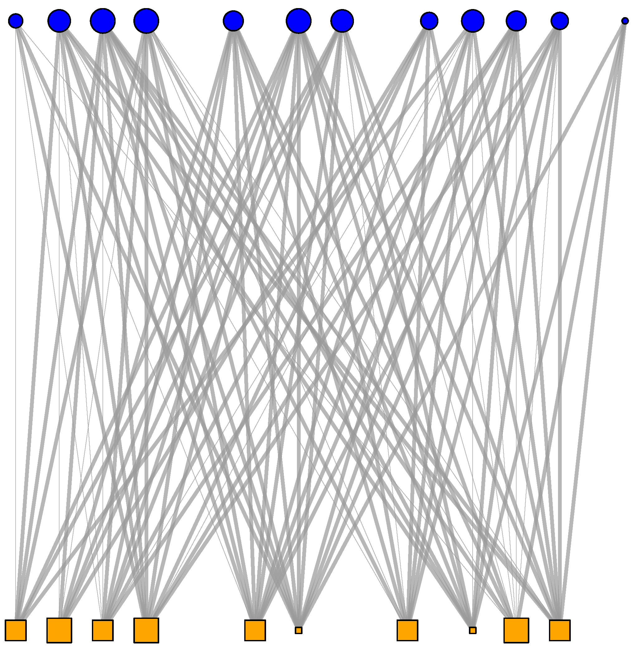
Affiliation networks, with their bipartite structure, show structural asymmetry: actors and events form two separate node sets with fixed roles (e.g., users and movies in rating networks), and links occur only between the sets. This differs from one-mode networks, where all nodes are of the same type and can connect to each other. However, symmetric patterns can still appear in affiliation networks. For example, users with similar attributes (e.g., age or genre preference) often choose events (e.g., movies) with similar attributes, creating a form of symmetry in cross-set links. Affiliation networks can also include edge weights. For example, in a user–event network, edge weights may represent how many times a user attended an event. Heavier weights show stronger relationships (e.g., frequent participation), while lighter weights show weaker relationships (e.g., attending only once). Using the MovieLens 100K dataset [37], we build a movie rating network with 88 users and 55 movies, as detailed analysis is provided in Section 5.2. Figure 1 visualizes the network topology by including the top $10\%$ of users and top $20\%$ of movies. User and movie nodes are shown as blue circles and orange squares, respectively. Node size is scaled logarithmically by degree. Edge width and opacity represent connection strength.

In this paper, we introduce the Generalized Logistic Affiliation Network (GLAN) model, a novel approach for analyzing affiliation networks that incorporates node attributes. GLAN builds on foundational models such as the $\beta$ model. These earlier models established a basis for understanding network structures but they often fail to integrate three critical elements within a unified framework. The three elements are degree heterogeneity, covariate effects and the distinct characteristics of two-mode networks. GLAN addresses this challenge by adopting the $\beta$ model’s approach to degree heterogeneity and extending it to bipartite structures. It employs a multinomial logistic link function to effectively manage discrete edge weights. This function enhances the interpretability of actor–event relationships. Additionally, GLAN incorporates both actor-level and event-level covariates. In this way it captures essential homophily effects. These effects are vital for understanding user interactions in real-world contexts. A key innovation of GLAN is its simultaneous consideration of degree heterogeneity, node attributes, and symmetric interaction patterns in bipartite networks. Furthermore, our model offers theoretical guarantees in the asymptotic regime, balancing flexibility and statistical rigor. Theoretical properties are established under asymptotic conditions where both the number of actors and events grows large, ensuring model reliability beyond empirical fit. Our main contributions are as follows:

1

Model Formulation: We formulate the GLAN model by incorporating node attributes with three key parameters: actor activeness, event popularity, and additional factors for actor–event interactions. We apply the GLAN model to analyze a movie-rating network. In this context, actor activeness is linked to user engagement, which is reflected in frequent ratings, while event popularity is measured through average ratings and review volume. Interaction factors, such as user demographics and genre preferences, provide insights into user rating behaviors. For more details, refer to Section 4.4.

2

Parameter Estimation: We estimate the GLAN model’s homophily parameters $\mathit{\gamma }$, degree heterogeneity parameters $\mathit{\alpha }$ and $\mathit{\beta }$ using the maximum likelihood estimation method. A stepwise optimization strategy is adopted. Given $\mathit{\gamma }$, the conditional maximum likelihood method is used to separately estimate $\mathit{\alpha }$ and $\mathit{\beta }$. Newton’s method is employed to compute the derivatives of the log-likelihood Function (2) in Section 3 to obtain the estimators ${\widehat{\mathit{\alpha }}}_{\mathit{\gamma }}$ and ${\widehat{\mathit{\beta }}}_{\mathit{\gamma }}$. These estimators are then iteratively used to optimize $\mathit{\gamma }$ until convergence. The existence and convergence of the estimators are verified by the Newton–Kantorovich conditions [38]. Under mild assumptions, as the number of actors and events increases, the maximum likelihood estimators (MLEs) of degree heterogeneity and homophily parameters converge to multivariate normal distributions, as confirmed by large sample theory.

3

Model Validation: Through simulations and empirical applications on the MovieLens 100K Dataset [37], we demonstrate the effectiveness and robustness of the GLAN model in capturing and analyzing affiliation networks.

The remainder of this paper is structured as follows: Section 2 details the structure of the GLAN model and the roles of its parameters. Section 3 discusses parameter estimation using the maximum likelihood method. Section 4 explores the asymptotic properties of the MLEs. Section 5 presents simulations and real-world data applications. Finally, Section 6 discusses the findings, limitations, and future research directions. All technical proofs are provided in the Appendix A.

2. GLAN Model with Node Attributes

Consider a weighted affiliation network $\mathcal{G}=([m],[n],\mathcal{W},\mathcal{Z})$, where $[m]:=\{1,2,\dots ,m\}$ represents the set of actors and $[n]:=\{1,2,\dots ,n\}$ represents the set of events. In this network, edges exist only between actors and events. For simplicity, we assume that $m\ge n$. The edge weight $a_{i,j}$ in the adjacency matrix $A\in {\mathbb{R}}^{m\times n}$ is drawn from the discrete set $\{0,1,\dots ,q\}\subset \mathcal{W}$, where q is a positive integer with $q\ge 2$. The edge weight $a_{i,j}$ quantifies the strength of the connection between actor $i\in [m]$ and event $j\in [n]$. For example, in a musician–concert affiliation network, a high $a_{i,j}$ for a particular musician and concert suggests that the musician plays a significant role in the concert, possibly as the headline act. Additionally, the matrix $\mathcal{Z}\in {\mathbb{R}}^{p\times mn}$ contains covariates. Each element $Z_{i,j}\in {\mathbb{R}}^p$ is a p-dimensional vector encoding essential features of an actor’s event participation. Specifically, it includes expressions like $|X_{k,i}-Y_{l,j}|$, which measures the difference or similarity between the k-th attribute of actor i and the l-th attribute of event j. Furthermore, $X_{k,i}\times Y_{l,j}$ reflects the interactive influence between the two attributes. For instance, consider the musical genre as an attribute. If a highly skilled jazz musician (where $X_{k,i}$ is large for the jazz genre) performs at a jazz concert (where $Y_{l,j}$ is prominent for the jazz genre), then $|X_{k,i}-Y_{l,j}|$ will be minimal, indicating a good alignment. Meanwhile, $X_{k,i}\times Y_{l,j}$ captures how this alignment influences the concert’s success or popularity. When both the actor’s proficiency in the relevant attribute and the event’s focus on that attribute are strong, the product suggests a higher likelihood of attracting a larger audience.

In this paper, we present a GLAN model, which integrates degree sequences and covariates as sufficient statistics. For each actor–event pair $(i,j),$ where $i\in [m],j\in [n]$, the probability distribution of the weight $a_{i,j}$, derived from the adjacency matrix A is defined as follows:

$$P(a_{i,j}=a)={\displaystyle \frac{exp\left\{a({\alpha }_i+{\beta }_j+Z_{ij}^{\top }\gamma )\right\}}{{\sum }_{k=0}^{q}exp\left\{k({\alpha }_i+{\beta }_j+Z_{ij}^{\top }\gamma )\right\}}},a\in \mathcal{W}.$$

(1)

In the GLAN model (1), ${\alpha }_i$ and ${\beta }_j$ represent actors’ activity levels and events’ popularity, respectively, while the vector $\mathit{\gamma }$ captures additional factors influencing the strength of the link between them. Our model (1) extends the renowned $\beta$ model [39] that emphasizes degree sequences. By integrating degree sequences and covariates as sufficient statistics, the enhanced model (1) allows for a detailed analysis of actor–event interactions, accounting for the homogeneous phenomenon caused by their attributes. It is particularly relevant for applications such as online shopping platforms, where relationship weights are influenced by user demographics, product characteristics, and transaction details. This approach affords a deeper understanding of the affiliation network by evaluating not only the frequency of interactions but also the underlying qualities and similarities that foster links.

Moreover, the structure of the GLAN model (1) remains invariant under a linear transformation of the parameters $(\mathit{\alpha },\mathit{\beta })$ to $(\mathit{\alpha }-c,\mathit{\beta }+c)$ for any non-zero constant c, ensuring model consistency. For the purposes of identifiability and to simplify asymptotic analysis, we set ${\beta }_n=0$. Specifically, this choice of constraint does not affect the intrinsic properties of the model or the estimation of relative differences between parameters. Its sole purpose is to anchor the parameter space for identifiability. The asymptotic variances and covariances derived for the parameter estimators, and consequently all subsequent statistical inference, are conditional on this specific constraint. Notably, inference on contrasts between parameters remains valid and is invariant to the particular node selected for the constraint.

3. Estimation

In this paper, we use the maximum likelihood method to estimate the parameters of the GLAN model in Equation (1). Let $\mathit{\theta }={(\mathit{\alpha },\mathit{\beta })}^{\top }$ and $\mathit{\gamma }$ represent the unknown homophily and heterogeneity parameter vectors, respectively. The estimators $\widehat{\mathit{\theta }}={(\widehat{\mathit{\alpha }},\widehat{\mathit{\beta }})}^{\top }$ and $\widehat{\mathit{\gamma }}$ are obtained by optimizing the log-likelihood function of the GLAN model in Equation (1):

$$\begin{array}{cc}\hfill log\mathcal{L}(\mathit{\theta },\mathit{\gamma }\mid A\})& =\sum _{i=1}^m\sum _{j=1}^n{a}_{i,j}{Z}_{i,j}^{\top }\gamma +\sum _{i=1}^m{d}_i{\alpha }_i+\sum _{j=1}^n{b}_j{\beta }_j\hfill \\ \hfill & -\sum _{i=1}^m\sum _{j=1}^{n}log\left(\sum _{k=0}^{q}exp\left\{k({\alpha }_i+{\beta }_j+Z_{i,j}^{\top }\gamma )\right\}\right),\hfill \end{array}$$

(2)

where $d_i={\sum }_{j=1}^n{a}_{i,j}$ and $b_j={\sum }_{i=1}^m{a}_{i,j}$ are the actor and event degrees for $i\in [m]$ and $j\in [n]$, respectively. Based on the above likelihood Function (2), we then derive the following score equations:

$$\begin{array}{cc}\hfill F_i(\mathit{\theta },\mathit{\gamma })& =d_i-\sum _{k=1}^n\sum _{a=0}^q{\displaystyle \frac{aexp\left\{a({\alpha }_i+{\beta }_k+Z_{i,j}^{\top }\gamma )\right\}}{{\sum }_{a=0}^{q}exp\left\{a({\alpha }_i+{\beta }_k+Z_{i,j}^{\top }\gamma )\right\}}},i\in [m],\hfill \\ \hfill F_{m+j}(\mathit{\theta },\mathit{\gamma })& =b_j-\sum _{k=1}^m\sum _{a=0}^q{\displaystyle \frac{aexp\left\{a({\alpha }_k+{\beta }_j+Z_{i,j}^{\top }\gamma )\right\}}{{\sum }_{a=0}^{q}exp\left\{a({\alpha }_k+{\beta }_j+Z_{i,j}^{\top }\gamma )\right\}}},j\in [n-1],\hfill \\ \hfill Q_k(\mathit{\theta },\mathit{\gamma })& =\sum _{i=1}^m\sum _{j=1}^n{z}_{i,j,k}(a_{i,j}-\sum _{a=0}^q{\displaystyle \frac{aexp\left\{a({\alpha }_i+{\beta }_j+Z_{i,j}^{\top }\gamma )\right\}}{{\sum }_{a=0}^{q}exp\left\{a({\alpha }_i+{\beta }_j+Z_{i,j}^{\top }\gamma )\right\}}}),k\in [p].\hfill \end{array}$$

(3)

Here, $z_{i,j,k}$ represents k-th element of p-dimensional attribute vector $Z_{i,j}$, which characterizes the k-th attribute characteristic between actor i’s participation in event j. Define $F(\mathit{\theta })={(F_1(\mathit{\theta },\mathit{\gamma }),\dots ,F_{m+n-1}(\mathit{\theta },\mathit{\gamma }))}^{\top }$ and $F_{\mathit{\gamma }}(\mathit{\theta })={(F_{\mathit{\gamma },1}(\mathit{\theta },\mathit{\gamma }),\dots ,F_{\mathit{\gamma },m+n-1}(\mathit{\theta },\mathit{\gamma }))}^{\top }$, where $F_{\gamma ,i}(\mathit{\theta })$ represents the value of $F_i(\mathit{\theta },\mathit{\gamma })$ with $\mathit{\gamma }$ fixed. Additionally, define

$$Q(\mathit{\theta },\mathit{\gamma })={(Q_1(\mathit{\theta },\mathit{\gamma }),\dots ,Q_p(\mathit{\theta },\mathit{\gamma }))}^{\top }$$

and

$$Q_c(\mathit{\gamma })=(Q_{c,1}({\widehat{\mathit{\theta }}}_{\mathit{\gamma }},\mathit{\gamma }),\dots ,Q_{c,p}{({\widehat{\mathit{\theta }}}_{\mathit{\gamma }},\mathit{\gamma })}^{\top },$$

where $Q_{c,i}({\widehat{\mathit{\theta }}}_{\mathit{\gamma }},\mathit{\gamma })$ is the value of $Q_i({\widehat{\mathit{\theta }}}_{\mathit{\gamma }},\mathit{\gamma })$ when ${\widehat{\mathit{\theta }}}_{\mathit{\gamma }}$ is the solution to $F_{\gamma }(\mathit{\theta })=0$ for $i\in [p]$. Solving the following system of equations:

$$\begin{array}{cc}\hfill & F(\mathit{\theta },\mathit{\gamma })=0,F_{\mathit{\gamma }}(\mathit{\theta })=0,\hfill \\ \hfill & Q({\widehat{\mathit{\theta }}}_{\mathit{\gamma }},\mathit{\gamma })=0,Q_c(\mathit{\gamma })=0\hfill \end{array}$$

(4)

yields the MLEs of $\mathit{\theta }$ and $\mathit{\gamma }$, respectively. The stepwise maximum likelihood estimation procedure is shown in Algorithm 1.   

Algorithm 1: The stepwise maximum likelihood estimation procedure

Input: Initial parameters ${\gamma }_0$, ${\theta }_0$; Convergence threshold $\epsilon$

Output: Parameter estimates $\widehat{\theta }$, $\widehat{\gamma }$

1 Initialize parameters ${\gamma }^{(0)}={\gamma }_0$, ${\theta }^{(0)}={\theta }_0$, and set iteration counter $k=0$ 2 Fix $\gamma ={\gamma }^{(k)}$. Use Newton’s method to solve the system $F_{\gamma }(\theta )=0$, obtaining the current estimate ${\theta }^{(k)}$ 3 Using the current parameters ${\theta }^{(k)}$ and ${\gamma }^{(k)}$, compute the function value $Q_c({\gamma }^{(k)})$ and its Jacobian matrix ${\left.{\displaystyle \frac{\partial Q_c}{\partial \gamma }}\right|}_{\gamma ={\gamma }^{(k)}}$ 4 Update the homophily parameter using Newton’s method: ${\gamma }^{(k+1)}={\gamma }^{(k)}-{\left[{\displaystyle \frac{\partial Q_c}{\partial \gamma }}\right]}^{-1}·Q_c({\gamma }^{(k)})$ 5 Check convergence If $\parallel {\gamma }^{(k+1)}-{\gamma }^{(k)}\parallel <\epsilon$, proceed to step 6; Otherwise, set $k=k+1$ and return to step 2 6 Return the final parameter estimates $\widehat{\theta }={\theta }^{(k)}$ and $\widehat{\gamma }={\gamma }^{(k)}$

4. Asymptotic Results

In this section, we analyze the asymptotic behavior of MLEs for the parameters in the GLAN model, as given in Equation (1). Our primary focus is on the neighborhood of the true parameter vectors, denoted by ${\mathit{\theta }}^{*}={({\mathit{\alpha }}^{*},{\mathit{\beta }}^{*})}^{\top }$ and ${\mathit{\gamma }}^{*}$. This neighborhood is defined by a specific bound that involves these parameters and the elements of the covariance matrix Z. Let $Q_{m,n},q_{m,n}$, and $Z_{max}:={\parallel Z_{i,j}\parallel }_{\infty }$ represent any positive numbers. The bound is expressed as follows:

$$\parallel {\alpha }_i^{*}+{\beta }_j^{*}{\parallel }_{\infty }\le Q_{m,n},{\parallel Z_{i,j}^{\top }{\mathit{\gamma }}^{*}\parallel }_{\infty }\le Z_{max}{q}_{m,n},$$

The parameter space $\Theta$ is then characterized as follows: for all $i\in [m],j\in [n]$:

$$\Theta =\{(\mathit{\alpha },\mathit{\beta },\mathit{\gamma }):\parallel {\alpha }_i+{\beta }_j{\parallel }_{\infty }\le Q_{m,n}+{ϵ}_{m,n},\parallel Z_{i,j}^{\top }\mathit{\gamma }{\parallel }_{\infty }\le Z_{max}{q}_{m,n}+{ϵ}_{m,n}\},$$

(5)

where ${ϵ}_{m,n}=O(\sqrt{{\displaystyle \frac{logm}{n}}})$ is an arbitrarily small value.

4.1. Characterization of the Fisher Information Matrix

In the analysis of affiliation network data, understanding the asymptotic properties of the MLE is crucial for hypothesis testing, prediction, and model validation. Classical asymptotic theory suggests that as the number of observed data increases, the MLE converges to a normal distribution centered around the true parameters, with its covariance determined by the inverse of the Fisher information matrix (FIM). However, deriving the inverse of the FIM can be complex. To address this, ref. [22] introduced a specialized matrix category, similar to the FIM, for analyzing the asymptotic behavior of the MLE. They defined a matrix $V\in {\mathcal{L}}_{m,n}(q,Q)$, a $(m+n-1)\times (m+n-1)$ matrix that satisfies specific criteria, making it diagonally dominant, symmetric, and nonnegative. For two positive numbers, q and Q, the matrix V has the following properties:

$$\begin{array}{c}q\le v_{i,i}-\sum _{j=m+1}^{m+n-1}{v}_{i,j}\le Q,i=1,\dots ,m;v_{m+n,m+n}:=\sum _{i=1}^{m+n-1}{v}_{m+n,i},\hfill \\ v_{i,j}=0,i,j=1,\dots ,m,i\ne j,\hfill \\ v_{i,j}=0,i,j=m+1,\dots ,m+n-1,i\ne j,\hfill \\ q\le v_{i,j}=v_{j,i}\le Q,i=1,\dots ,m,j=m+1,\dots ,m+n-1,\hfill \\ v_{i,i}=\sum _{k=1}^m{v}_{k,i}=\sum _{k=1}^m{v}_{i,k},i=m+1,\dots ,m+n-1.\hfill \end{array}$$

(6)

To simplify the inversion of V, ref. [22] introduced an approximation matrix S to estimate $V^{-1}$. The structure of S is given by the following equation:

$$s_{i,j}=\left\{\begin{array}{cc}{\displaystyle \frac{{\delta }_{i,j}}{v_{i,i}}}+{\displaystyle \frac{1}{v_{m+n,m+n}}},\hfill & i,j=1,\dots ,m,\hfill \\ -{\displaystyle \frac{1}{v_{m+n,m+n}}},\hfill & i=1,\dots ,m,j=m+1,\dots ,m+n-1,\hfill \\ -{\displaystyle \frac{1}{v_{m+n,m+n}}},\hfill & i=m+1,\dots ,m+n-1,j=1,\dots ,m,\hfill \\ {\displaystyle \frac{{\delta }_{i,j}}{v_{i,i}}}+{\displaystyle \frac{1}{v_{m+n,m+n}}},\hfill & i,j=m+1,\dots ,m+n-1.\hfill \end{array}\right.$$

(7)

Here, ${\delta }_{i,j}$ represents the Kronecker function. This approach reduces computational complexity and effectively handles the high-dimensional structures that are characteristic of network data analysis.

For any fixed $\mathit{\gamma }$, we denote the Jacobian matrix of $F_{\mathit{\gamma }}(\mathit{\theta })$ with respect to $\mathit{\theta }$ as

$${\displaystyle \frac{\partial F_{\mathit{\gamma }}(\mathit{\theta })}{\partial {\mathit{\theta }}^{\top }}}={\left({\displaystyle \frac{\partial F_{\mathit{\gamma },i}(\mathit{\theta })}{\partial {\mathit{\theta }}_j}}\right)}_{i,j=1}^{m+n-1,m+n-1},$$

where

$${\displaystyle \frac{\partial F_{\mathit{\gamma },i}(\mathit{\theta })}{\partial {\mathit{\theta }}_j}}=\left\{\begin{array}{cc}{\displaystyle \frac{\partial F_{\mathit{\gamma },i}(\mathit{\theta })}{\partial {\alpha }_k}},\hfill & j=k\in [m];\hfill \\ \\ {\displaystyle \frac{\partial F_{\mathit{\gamma },i}(\mathit{\theta })}{\partial {\beta }_k}},\hfill & j=m+k\in [m+n-1]\setminus [m].\hfill \end{array}\right.$$

Further, let ${\pi }_{i,j}={\alpha }_i+{\beta }_j+Z_{i,j}^{\top }\mathit{\gamma }.$ By (3), we obtain

$${\displaystyle \frac{\partial F_{\mathit{\gamma },i}(\mathit{\theta })}{\partial {\mathit{\theta }}_j}}=\left\{\begin{array}{c}0,\mathrm{if}i\ne j,i,j\in [m]\mathrm{or}i,j\in [m+n-1]\setminus [m];\hfill \\ \\ -\sum _{k=1}^n{\displaystyle \frac{{\sum }_{0\le t\ne s\le q}{(t-s)}^2{e}^{(t+s){\pi }_{i,k}}}{{({\sum }_{a=0}^q{e}^{a{\pi }_{i,j}})}^2}},\mathrm{if}i=j\in [m];\hfill \\ \\ -{\displaystyle \frac{{\sum }_{0\le t\ne s\le q}{(t-s)}^2{e}^{(t+s){\pi }_{k,l}}}{{({\sum }_{a=0}^q{e}^{a{\pi }_{k,l}})}^2}},\mathrm{if}i=k\in [m],j=m+l\in [m+n-1]\setminus [m]\hfill \\ \mathrm{or}i=k+m\in [m+n-1]\setminus [m],j=l\in [m];\hfill \\ \\ -\sum _{k=1}^m{\displaystyle \frac{{\sum }_{0\le t\ne s\le q}{(t-s)}^2{e}^{(t+s){\pi }_{k,j}}}{{({\sum }_{a=0}^q{e}^{a{\pi }_{k,j}})}^2}},\mathrm{if}i=j\in [m+n-1]\setminus [m].\hfill \\ \end{array}\right.$$

(8)

Since ${({\sum }_{a=0}^q{e}^{a{\pi }_{k,l}})}^2={\sum }_{a=0}^q{e}^{2a{\pi }_{k,l}}+{\sum }_{0\le t\ne s\le q}{e}^{(t+s){\pi }_{k,l}},$ by (5), we have

$$\sum _{0\le t\ne s\le q}{e}^{(t+s){\pi }_{k,l}}\le {(\sum _{a=0}^q{e}^{a{\pi }_{k,l}})}^2\le \sum _{0\le t\ne s\le q}{e}^{(t+s){\pi }_{k,l}}(1+b_{m,n}),$$

where $b_{m,n}:=e^{\parallel {\pi }_{k,l}{\parallel }_{\infty }}=O(e^{Q_{m,n}+Z_{max}{q}_{m,n}}).$ Further, we obtain

$$\begin{array}{cc}\hfill {\displaystyle \frac{{\sum }_{0\le t\ne s\le q}{e}^{(t+s){\pi }_{k,l}}}{{\sum }_{0\le t\ne s\le q}{e}^{(t+s){\pi }_{k,l}}(1+b_{m,n})}}& \le {\displaystyle \frac{{\sum }_{0\le t\ne s\le q}{(t-s)}^2{e}^{(t+s){\pi }_{k,l}}}{{({\sum }_{a=0}^q{e}^{a{\pi }_{k,l}})}^2}}\hfill \\ \hfill & \le {\displaystyle \frac{{max}_{t\ne s}{(t-s)}^2{\sum }_{0\le t\ne s\le q}{e}^{(t+s){\pi }_{k,l}}}{{\sum }_{0\le t\ne s\le q}{e}^{(t+s){\pi }_{k,l}}}}=q^2.\hfill \end{array}$$

(9)

From (6) and (9), we have

$$\begin{array}{c}\hfill -{\displaystyle \frac{\partial F_{\mathit{\gamma }}(\mathit{\theta })}{\partial {\mathit{\theta }}^{\top }}}\in {\mathcal{L}}_{m,n}\left({\displaystyle \frac{1}{1+b_{m,n}}},q^2\right).\end{array}$$

(10)

Next, we delve into the Jacobian matrix of $Q_c(\mathit{\gamma })$ on $\mathit{\gamma }$ to analyze the asymptotic properties of $\mathit{\gamma }$. By (4) and the compound function derivation law, we have

$$\begin{array}{c}\hfill 0={\displaystyle \frac{\partial F_{\mathit{\gamma }}({\widehat{\mathit{\theta }}}_{\mathit{\gamma }})}{\partial {\mathit{\gamma }}^{\top }}}={\displaystyle \frac{\partial F({\widehat{\mathit{\theta }}}_{\mathit{\gamma }},\mathit{\gamma })}{\partial {\mathit{\theta }}^{\top }}}{\displaystyle \frac{\partial {\widehat{\mathit{\theta }}}_{\mathit{\gamma }}}{{\mathit{\gamma }}^{\top }}}+{\displaystyle \frac{\partial F({\widehat{\mathit{\theta }}}_{\mathit{\gamma }},\mathit{\gamma })}{\partial {\mathit{\gamma }}^{\top }}},\\ \hfill {\displaystyle \frac{\partial Q_c(\mathit{\gamma })}{\partial {\mathit{\gamma }}^{\top }}}={\displaystyle \frac{\partial Q({\widehat{\mathit{\theta }}}_{\mathit{\gamma }},\mathit{\gamma })}{\partial {\mathit{\theta }}^{\top }}}{\displaystyle \frac{\partial {\widehat{\mathit{\theta }}}_{\mathit{\gamma }}}{{\mathit{\gamma }}^{\top }}}+{\displaystyle \frac{\partial Q({\widehat{\mathit{\theta }}}_{\mathit{\gamma }},\mathit{\gamma })}{\partial {\mathit{\gamma }}^{\top }}}.\end{array}$$

(11)

By (11), we have

$${\displaystyle \frac{\partial Q_c(\mathit{\gamma })}{\partial {\mathit{\gamma }}^{\top }}}={\displaystyle \frac{\partial Q({\widehat{\mathit{\theta }}}_{\mathit{\gamma }},\mathit{\gamma })}{\partial {\mathit{\gamma }}^{\top }}}-{\displaystyle \frac{\partial Q({\widehat{\mathit{\theta }}}_{\mathit{\gamma }},\mathit{\gamma })}{\partial {\mathit{\theta }}^{\top }}}{\left[{\displaystyle \frac{\partial F({\widehat{\mathit{\theta }}}_{\mathit{\gamma }},\mathit{\gamma })}{\partial {\mathit{\theta }}^{\top }}}\right]}^{-1}{\displaystyle \frac{\partial F({\widehat{\mathit{\theta }}}_{\mathit{\gamma }},\mathit{\gamma })}{\partial {\mathit{\gamma }}^{\top }}},$$

where

$${\displaystyle \frac{\partial Q({\widehat{\mathit{\theta }}}_{\mathit{\gamma }},\mathit{\gamma })}{\partial {\mathit{\gamma }}^{\top }}}:={\displaystyle \frac{\partial Q(\mathit{\theta },\mathit{\gamma })}{\partial {\mathit{\gamma }}^{\top }}}{|}_{\mathit{\theta }={\widehat{\mathit{\theta }}}_{\mathit{\gamma }},\mathit{\gamma }=\mathit{\gamma }},{\displaystyle \frac{\partial F({\widehat{\mathit{\theta }}}_{\mathit{\gamma }},\mathit{\gamma })}{\partial {\mathit{\theta }}^{\top }}}:={\displaystyle \frac{\partial F(\mathit{\theta },\mathit{\gamma })}{\partial {\mathit{\theta }}^{\top }}}{|}_{\mathit{\theta }={\widehat{\mathit{\theta }}}_{\mathit{\gamma }},\mathit{\gamma }=\mathit{\gamma }}.$$

Since ${\widehat{\mathit{\theta }}}_{\mathit{\gamma }}$ does not have a closed form, it is difficult to directly verify the conditions on the Jacobian matrix $\partial Q_c(\mathit{\gamma })/\partial {\mathit{\gamma }}^{\top }$. To facilitate the analysis, we define $H(\mathit{\theta },\mathit{\gamma }):=\partial Q_c(\mathit{\gamma })/\partial {\mathit{\gamma }}^{\top }$ as the FIM of the concentrated likelihood function $\mathcal{L}(\mathit{\gamma }\mid A,\mathit{\theta })$. Following the approach outlined in [34], when $\mathit{\theta }\in B({\mathit{\theta }}^{*},{ϵ}_{m,n})$ with ${ϵ}_{m,n}=O(\sqrt{{\displaystyle \frac{logm}{n}}})$, we approximate

$$\begin{array}{c}\hfill {\displaystyle \frac{1}{{(m+n-1)}^2}}H{(\mathit{\theta },{\mathit{\gamma }}^{*})}_{i,j}={\displaystyle \frac{1}{{(m+n-1)}^2}}H{({\mathit{\theta }}^{*},{\mathit{\gamma }}^{*})}_{i,j}+o(1).\end{array}$$

(12)

Thus, there exists a constant

$$\begin{array}{c}\hfill k_{m,n}=\sqrt{\rho }\times \underset{\mathit{\theta }\in B({\mathit{\theta }}^{*},{ϵ}_{m,n,1})}{sup}{\displaystyle \frac{1}{{\lambda }_{min}^{1/2}(\mathit{\theta })}}.\end{array}$$

(13)

where ${\lambda }_{min}(\mathit{\theta })$ is the smallest eigenvalue of ${\displaystyle \frac{1}{{(m+n-1)}^2}}{H}^{\top }(\mathit{\theta },{\mathit{\gamma }}^{*})H(\mathit{\theta },{\mathit{\gamma }}^{*})$. Consequently, we can establish that

$$\begin{array}{c}\hfill \underset{\mathit{\theta }\in B({\mathit{\theta }}^{*},{ϵ}_{m,n,1})}{sup}{\parallel H^{-1}(\mathit{\theta },{\mathit{\gamma }}^{*})\parallel }_{\infty }\le {\displaystyle \frac{k_{m,n}}{{(m+n-1)}^2}}.\end{array}$$

(14)

In this context, for $\mathit{\theta }\in B({\mathit{\theta }}^{*},{ϵ}_{m,n,1})$, since ${\lambda }_{min}(\mathit{\theta })$ is the smallest eigenvalue of ${(m+n-1)}^{-2}{H}^{\top }(\mathit{\theta },{\mathit{\gamma }}^{*})H(\mathit{\theta },{\mathit{\gamma }}^{*})$, it implies that ${\lambda }_{min}^{-1}(\mathit{\theta })$ is the largest eigenvalue of ${(m+n-1)}^2{(H^{\top }(\mathit{\theta },{\mathit{\gamma }}^{*})H(\mathit{\theta },{\mathit{\gamma }}^{*}))}^{-1}$. Therefore, we have

$$\begin{array}{cc}\hfill \parallel H^{-1}(\mathit{\theta },{\mathit{\gamma }}^{*}){\parallel }_2& ={\displaystyle \frac{1}{{(m+n-1)}^2{\lambda }_{min}^{1/2}(\mathit{\theta })}}\hfill \\ \hfill & \le \underset{\mathit{\theta }\in B({\mathit{\theta }}^{*},{ϵ}_{m,n,1})}{sup}{\displaystyle \frac{1}{{(m+n-1)}^2{\lambda }_{min}^{1/2}(\mathit{\theta })}}.\hfill \end{array}$$

Considering the relationship between the spectral norm and the infinity norm of matrices, it follows that

$$\begin{array}{cc}\hfill \parallel H^{-1}(\mathit{\theta },{\mathit{\gamma }}^{*}){\parallel }_{\infty }& \le \sqrt{\rho }{\parallel H^{-1}(\mathit{\theta },{\mathit{\gamma }}^{*})\parallel }_2\hfill \\ \hfill & \le {\displaystyle \frac{\sqrt{\rho }}{{(m+n-1)}^2}}\underset{\mathit{\theta }\in B({\mathit{\theta }}^{*},{ϵ}_{m,n,1})}{sup}{\displaystyle \frac{1}{{\lambda }_{min}^{1/2}(\mathit{\theta })}}\hfill \\ \hfill & \le {\displaystyle \frac{k_{m,n}}{{(m+n-1)}^2}}.\hfill \end{array}$$

4.2. Consistency

In the GLAN model (1), we employ a stepwise optimization strategy to estimate the parameters $\mathit{\theta }=(\mathit{\alpha },\mathit{\beta })$ and $\mathit{\gamma }$, effectively handling nonlinear complexities. First, for any fixed $\mathit{\gamma }$, we estimate $\mathit{\theta }$ separately via the conditional maximum likelihood method to reduce the multi-parameter estimation challenge. The estimators ${\mathit{\theta }}_{\mathit{\gamma }}$ are obtained by applying Newton’s method to calculate the first and second derivatives of the log-likelihood Function (2) with $\mathit{\gamma }$ fixed. Next, we iteratively optimize $\mathit{\gamma }$ using these estimators until convergence is achieved. The existence and convergence of these estimators are guaranteed by satisfying the Newton–Kantorovich conditions [38]. The consistency of the estimators is verified through large sample theory, which shows that the estimation error decreases as the sample size increases, ensuring accurate parameter estimation and theoretical validity. The existence and consistency of the MLEs $\widehat{\mathit{\theta }}$ and $\widehat{\mathit{\gamma }}$, along with their proofs, are presented in Appendix A.

Theorem 1.

Assume that parameters $(\mathit{\theta },\mathit{\gamma })\in \Theta$ as defined in (5) and $k_{m,n}{b}_{m,n}^6=O{\left({\displaystyle \frac{n}{logm}}\right)}^{1/4}$. If $m/n=O(1)$, then with probability at least $1-C_1{m}^{-1}$, the MLEs $(\widehat{\mathit{\theta }},\widehat{\mathit{\gamma }})$ exist and satisfy

$$\begin{array}{cc}\hfill \parallel \widehat{\mathit{\theta }}-{\mathit{\theta }}^{*}{\parallel }_{\infty }& =O_p({\displaystyle \frac{{(1+b_{m,n})}^3}{n}}\sqrt{{\displaystyle \frac{logm}{m}}})=o_p(1),\hfill \end{array}$$

(15)

$$\begin{array}{cc}\hfill \parallel \widehat{\mathit{\gamma }}-{\mathit{\gamma }}^{*}{\parallel }_{\infty }& =O_p({\displaystyle \frac{k_{m,n}{(1+b_{m,n})}^3\sqrt{logm}}{m^{3/2}}})=o_p(1),\hfill \end{array}$$

(16)

where $C_1$ is a constant.

Remark 1. 

Theorem 1 establishes the existence and consistency of the MLEs $\widehat{\mathit{\theta }}$ and $\widehat{\mathit{\gamma }}$ under specific regularity conditions. It guarantees their existence with a probability of at least $1-C_1{m}^{-1}$, implying that the probability of non-existence decreases as the sample size m increases, enhancing practical applicability. The error bounds in (15) and (16) quantify the accuracy of the estimators. Specifically, (15) shows that the estimation error for ${\mathit{\theta }}^{*}$ decreases as the sample size m increases, where ${(1+b_{m,n})}^3/n$ reflects the effect of model complexity, and $\sqrt{{\displaystyle \frac{logm}{m}}}$ indicates improved convergence as both n and m grow. Similarly, (16) quantifies the convergence rate of $\widehat{\mathit{\gamma }}$ towards the true parameter ${\mathit{\gamma }}^{*}$. The term $k_{m,n}$ accounts for additional model complexity that affects ${\mathit{\gamma }}^{*}$, while the factor $m^{3/2}$ highlights the faster convergence with larger m. The conditions $k_{m,n}{b}_{m,n}^6=O{\left({\displaystyle \frac{n}{logm}}\right)}^{1/4}$ and $m/n=O(1)$ balance model complexity with sample scalability, ensuring estimator reliability and consistency in high-dimensional settings or under increasing model complexities.

4.3. Asymptotic Distribution of $\widehat{\theta }$

In this scetion, we explore the asymptotic distribution of $\widehat{\mathit{\theta }}$ as both the number of actors and events tends to infinity. The asymptotic variance of $\widehat{\mathit{\theta }}$ is influenced by the covariance structure of the observed node degrees. To begin our analysis, we focus on the asymptotic properties of the degree sequence, which is essential for understanding the asymptotic behavior of $\widehat{\mathit{\theta }}$.

Proposition 1. 

Let $\mathbf{g}={(d_1,\dots ,d_m,b_1,\dots ,b_{n-1})}^{\top }$ and $g_{m+n}=b_n$. If $m/n=O(1),1+b_{m,n}=O(\sqrt{n})$ as $m\to \infty$, then we have

$$(g_i-\mathbb{E}(g_i))/v_{i,i}^{1/2}\stackrel{d}{\to }\mathcal{N}(0,1),$$

(17)

where $g_i$ represents the i-th element of $\mathbf{g}$. Moreover, for any fixed $k\ge 1$, as $m\to \infty$, the vector formed by the first k elements of $S\{\mathbf{g}-\mathbb{E}(\mathbf{g})\}$ is asymptotically multivariate normal with mean zero and covariance matrix equal to the upper left $k\times k$ submatrix of $S=1/v_{m+n,m+n}^2+diag(1/v_{1,1}^2,\dots ,1/v_{m+n-1,m+n-1}^2)$ as defined in (7).

Remark 2. 

The covariance matrix of the centered degree sequence $\{\mathbf{g}-\mathbb{E}(\mathbf{g})\}$ is given by $V=-\partial F_{\mathit{\gamma }}(\mathit{\theta })/\partial {\mathit{\theta }}^{\top }\in {\mathcal{L}}_{m,n}\left(1/(1+b_{m,n}),q^2\right)$. This results in the bounds $n/(2(1+b_{m,n}))\le v_{i,i}\le m{q}^2/2$, for $i\in [m+n-1]$. According to the central limit theorem for boundary cases (see Loéve [40], p. 289), if $v_{i,i}$ diverges, the scaled deviations $v_{i,i}^{-1/2}(d_i-\mathbb{E}(d_i))$ and $v_{m+j,m+j}^{-1/2}(b_j-\mathbb{E}(b_j))$ converge in distribution to the standard normal distribution. The degree sequence $\mathbf{g}$ is crucial in understanding the behavior of the estimator $\widehat{\mathit{\theta }}$ as the sample size, reflected by the number of actors and events, approaches infinity. By exploring the asymptotic behavior of $\mathbf{g}$, we gain insights into the properties and distribution characteristics of the estimator $\widehat{\mathit{\theta }}$ in the limit. This analysis is fundamental to the asymptotic theory of the GLAN model (1), providing a deeper understanding of the estimator’s behavior in large sample settings.

We are now ready to depict the asymptotic behavior of $\widehat{\mathit{\theta }}$, with its proof presented in the Appendix A, as follows.

Theorem 2.

Suppose that the conditions stated in Theorem 1 are satisfied. If $k_{m,n}{(1+b_{m,n})}^6=O(n^{3/4}/\sqrt{logm}),$ then for any fixed $k\ge 1$, as $m\to \infty$, we have

$${\widehat{\mathit{\theta }}}_{[1:k]}-{\mathit{\theta }}_{[1:k]}\stackrel{d}{\to }\mathcal{N}(0,S_{[1:k,1:k]})$$

(18)

where ${\widehat{\mathit{\theta }}}_{[1:k]}$ and ${\mathit{\theta }}_{[1:k]}$ denote the first k elements of the respective vectors, and $S_{[1:k,1:k]}$ represents the upper left $k\times k$ submatrix of S as defined in (7).

Remark 3. 

Theorem 2 illustrates the asymptotic behavior of the estimator $\widehat{\mathit{\theta }}$, demonstrating that it converges to a multivariate normal distribution as the number of actors and events approaches infinity. The condition $k_{m,n}{(1+b_{m,n})}^6=O\left({\displaystyle \frac{n^{3/4}}{\sqrt{logm}}}\right)$ guarantees that the growth rate of the factor $k_{m,n}$, which indicates the underlying model complexity, is appropriately regulated by the factor ${(1+b_{m,n})}^6$. This balance is crucial for achieving asymptotic normality, ensuring that model complexity does not exceed the information available as m and n become large. The factor $k_{m,n}$, which is defined in (13) as the inverse of the minimum eigenvalue of a scaled Hessian, reflects the local curvature of the log-likelihood and significantly influences the estimator’s behavior. For a fixed $k\ge 1$ as $m\to \infty$, the estimator’s deviation converges to a normal distribution with covariance $S_{[1:k,1:k]}$. Proposition 1 correlates degree sequence analysis with Theorem 2, uncovering covariance matrix bounds and asymptotic normality in boundary scenarios. The matrix $S_{[1:k,1:k]}$ emphasizes the estimation accuracy across parameters, facilitating hypothesis tests and confidence intervals in affiliation networks. For example, an approximate $1-\alpha$ confidence interval for ${\theta }_i-{\theta }_j$ is provided by ${\widehat{\theta }}_i-{\widehat{\theta }}_j\pm Z_{1-\alpha /2}{(1/{\widehat{v}}_{i,i}+1/{\widehat{v}}_{j,j})}^{1/2}$, where $Z_{1-\alpha /2}$ represents the $1-\alpha$-quantile of the standard normal distribution, and ${\widehat{v}}_{i,i}$ and ${\widehat{v}}_{j,j}$ are the maximum likelihood estimates of $v_{i,i}$ and $v_{j,j}$ obtained by replacing all ${\theta }_i$ with their MLEs.

4.4. Asymptotic Distribution of $\widehat{\gamma }$

In this section, we first investigate the asymptotic properties of the term $S_{i,j}({\mathit{\theta }}^{*},{\mathit{\gamma }}^{*})$, which is defined as:

$$S_{i,j}({\mathit{\theta }}^{*},{\mathit{\gamma }}^{*})=\left(a_{i,j}-\mathbb{E}(a_{i,j})\right)\left(Z_{i,j}-{\displaystyle \frac{\partial Q({\mathit{\theta }}^{*},{\mathit{\gamma }}^{*})}{\partial {\mathit{\theta }}^{\top }}}{\left[{\displaystyle \frac{\partial F({\mathit{\theta }}^{*},{\mathit{\gamma }}^{*})}{\partial {\mathit{\theta }}^{\top }}}\right]}^{-1}{T}_{i,j}\right),$$

where $T_{i,j}$ is an $m+n-1$ dimensional column vector with the i-th and $m+j$-th elements equal to 1, and all other elements equal to 0. This analysis is crucial for grasping the distributional behavior of the estimator $\widehat{\mathit{\gamma }}$ as the number of actors and events tends to infinity. The variance of $\widehat{\mathit{\gamma }}$ is intrinsically related to the covariance structure within $S_{i,j}({\mathit{\theta }}^{*},{\mathit{\gamma }}^{*})$. Therefore, a detailed investigation of $S_{i,j}({\mathit{\theta }}^{*},{\mathit{\gamma }}^{\mathit{*}})$ is critical for elucidating the statistical properties of the estimator $\widehat{\mathit{\gamma }}$.

Proposition 2. 

If $m/n=O(1),1+b_{m,n}=O(n^{1/6})$ and $H({\mathit{\theta }}^{*},{\mathit{\gamma }}^{*})$ diverges, as $m\to \infty$, then we have

$${\displaystyle \frac{{\sum }_{i=1}^m{\sum }_{j=1}^{n-1}{S}_{i,j}({\mathit{\theta }}^{*},{\mathit{\gamma }}^{*})}{\sqrt{H({\mathit{\theta }}^{*},{\mathit{\gamma }}^{*})}}}\stackrel{d}{\to }\mathcal{N}(0,1),$$

(19)

where $H({\mathit{\theta }}^{*},{\mathit{\gamma }}^{*})$ is the value of $H(\mathit{\theta },\mathit{\gamma })={\displaystyle \frac{\partial Q(\mathit{\theta },\mathit{\gamma })}{\partial {\mathit{\gamma }}^{\top }}}$ at true parameter vector $({\mathit{\theta }}^{*},{\mathit{\gamma }}^{*})$.

Remark 4.

The proof of Proposition 2 is provided in the Appendix A. In the proof, we investigate the asymptotic behavior of the sum of $S_{i,j}({\mathit{\theta }}^{*},{\mathit{\gamma }}^{*})$ under specific conditions. The sum converges in distribution to a normal distribution, due to the independence and boundedness of each $S_{i,j}({\mathit{\theta }}^{*},{\mathit{\gamma }}^{*})$, which satisfies the requirements of the central limit theorem (Loéve [40], p. 289). First, each term $S_{i,j}({\mathit{\theta }}^{*},{\mathit{\gamma }}^{*})$ is derived independently, as it only depends on its respective $a_{i,j}$, ensuring the applicability of the central limit theorem. Second, the boundedness of $S_{i,j}({\mathit{\theta }}^{*},{\mathit{\gamma }}^{*})$ is confirmed by estimating the magnitude of the adjustments to $Q({\mathit{\theta }}^{*},{\mathit{\gamma }}^{*})$ made by $\partial Q({\mathit{\theta }}^{*},{\mathit{\gamma }}^{*})/\partial {\mathit{\theta }}^{\top }$, which remains sufficiently small as $m,n\to \infty$ with $1+b_{m,n}=O(n^{1/6})$. Finally, the covariance of the sum of $S_{i,j}({\mathit{\theta }}^{*},{\mathit{\gamma }}^{*})$ is equal to $H({\mathit{\theta }}^{*},{\mathit{\gamma }}^{*})$, a key quantity varying with m and n. This variation ensures the variance becomes large enough for effective application of the central limit theorem.

Let $\mu (t)={\displaystyle \sum _{a=0}^q}{\displaystyle \frac{a{e}^{at}}{{\sum }_{k=0}^q{e}^{kt}}}$, and ${\pi }_{i,j}^{*}={\alpha }_i^{*}+{\beta }_j^{*}+Z_{i,j}^{\top }{\mathit{\gamma }}^{*}.$ Denote ${\mu }^{\prime }({\pi }_{i,j}^{*})$ and ${\mu }^{″}({\pi }_{i,j}^{*})$ as the first and second derivatives of $\mu (t)$ with respect to t, evaluated at $t={\pi }_{i,j}^{*}$. Consider the limiting behavior of matrix $\overline{H}$ defined as

$$\overline{H}=\underset{m\to \infty }{lim}{\displaystyle \frac{1}{{(m+n-1)}^2}}H({\mathit{\theta }}^{*},{\mathit{\gamma }}^{*}),$$

where $H({\mathit{\theta }}^{*},{\mathit{\gamma }}^{*})$ is the value of $H(\mathit{\theta },\mathit{\gamma })={\displaystyle \frac{\partial Q(\mathit{\theta },\mathit{\gamma })}{\partial {\mathit{\gamma }}^{\top }}}$ at the true parameter vector $({\mathit{\theta }}^{*},{\mathit{\gamma }}^{*})$. Under these conditions, we can obtain the asymptotic distribution of parameter estimator $\widehat{\mathit{\gamma }}$. We formalize this in the following theorem.

Theorem 3.

Suppose the conditions in Proposition 2 hold. If $O(1+b_{m,n})=n^{1/36}/{(logm)}^{1/9},$ then for any fixed $k\ge 1$, as $m\to \infty$, we have

$$(m+n-1)(\widehat{\mathit{\gamma }}-{\mathit{\gamma }}^{*})\stackrel{d}{\to }\mathcal{N}({\overline{H}}^{-1}{B}_{*},H({\mathit{\theta }}^{*},{\mathit{\gamma }}^{*})),$$

(20)

where

$$B_{*}={\displaystyle \frac{1}{2(m+n-1)}}\sum _{k=1}^m\sum _{l=m+1}^{m+n-1}{Z}_{k,l}{\mu }^{″}({\pi }_{k,l}^{*})({\displaystyle \frac{1}{{\sum }_{l=m+1}^{m+n-1}{\mu }^{\prime }({\pi }_{k,l}^{*})}}+{\displaystyle \frac{1}{{\sum }_{k=1}^m{\mu }^{\prime }({\pi }_{k,l}^{*})}}).$$

Remark 5. 

The proof of Theorem 3 is presented in the Appendix A. Theorem 3 states that the scaled estimator $(m+n-1)(\widehat{\mathit{\gamma }}-{\mathit{\gamma }}^{*})$ converges in distribution to a normal distribution. The mean of this normal distribution involves a bias term ${\overline{H}}^{-1}{B}_{*}$, and the variance is $H({\mathit{\theta }}^{*},{\mathit{\gamma }}^{*})$. The bias term $B_{*}$ encapsulates the intricate relationships between the covariates $Z_{i,j}$ and the second derivatives of the nonlinear function $\mu ({\pi }_{i,j}^{*})$, reflecting the impact of second order interactions on estimation bias. To achieve unbiased inference, particularly for constructing confidence intervals and conducting hypothesis tests, it is essential to apply bias correction. Following the method by [41], a bias corrected estimator ${\widehat{\mathit{\gamma }}}_{bc}$ is recommended: ${\widehat{\mathit{\gamma }}}_{bc}=\widehat{\mathit{\gamma }}-{(m+n-1)}^{-1}{\overline{H}}^{-1}(\widehat{\mathit{\theta }},\widehat{\mathit{\gamma }}){\widehat{B}}_{*},$ where ${\widehat{B}}_{*}$ is a plug-in estimator for $B_{*}$, computed using the estimates $\widehat{\mathit{\beta }}$ and $\widehat{\mathit{\gamma }}.$ This correction is crucial for ensuring that the central limit theorem accurately describes the distribution of the estimator $\widehat{\mathit{\gamma }}$, accounting for the bias.

5. Numerical Studies

In this section, we present numerical experiments using synthetic data generated from the GLAN model (1), with discrete weights ($q=2$), to evaluate the performance of our MLEs. Additionally, we provide an example using the MovieLens 100K dataset [37].

5.1. Simulations

To examine the finite sample properties of Theorem 3, we conduct simulations on an affiliation network of size $(m,n)=(100,50)$ and $(120,70)$, respectively. The parameters are set as ${\alpha }_i^{*}=(m-i)L/(m-1)$ and ${\beta }_j^{*}=(n-j)L/(n-1)$, where $i\in [m],j\in [n]$, and $L\in \{0,log(logm)/m,\sqrt{logm}/m\}.$ Each node is assigned two independent covariates, $X_{k,i}$ and $Y_{l,j}$, sampled from a $Beta(2,2)$. For node pairs $(i,j)$, the covariates are defined as $Z_{i,j}=(|X_{k,i}-Y_{l,j}{|,X_{k,i}\times Y_{l,j})}^{\top }.$ The homophily parameter ${\mathit{\gamma }}^{*}={(1,1.5)}^{\top }$ encodes features of actor i’s participation in event $j.$

Based on Theorem 3, we assess the asymptotic distribution of

$${\widehat{\xi }}_{i,j}={\displaystyle \frac{{\widehat{\theta }}_i-{\widehat{\theta }}_j-({\theta }_i^{*}-{\theta }_j^{*})}{\sqrt{1/{\widehat{v}}_{i,i}+1/{\widehat{v}}_{j,j}}}}.$$

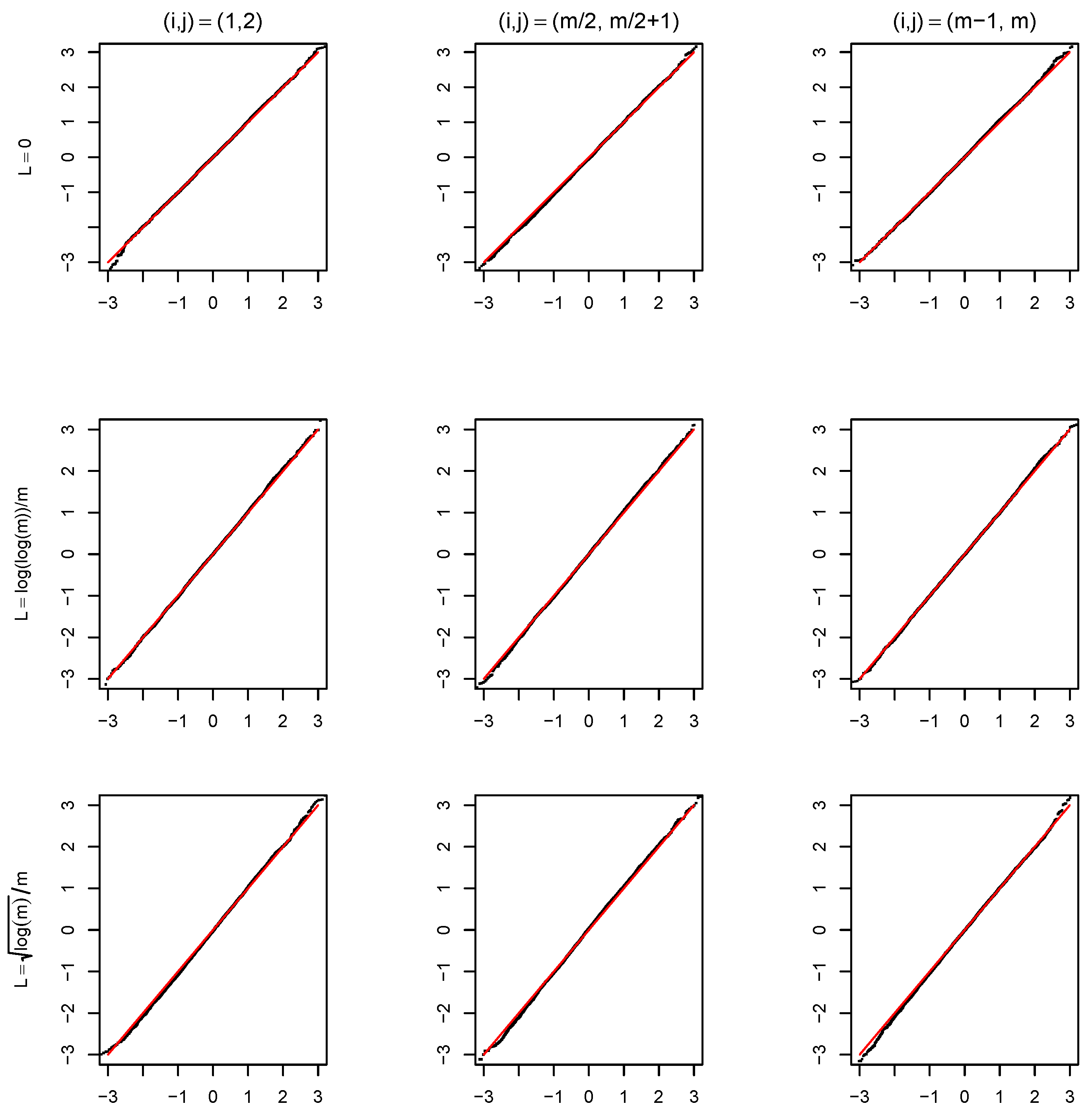
Here, ${\widehat{v}}_{i,i}$ is the estimate of $v_{i,i}$, obtained by substituting ${\widehat{\theta }}_i$ for ${\theta }_i^{*}$, where ${\theta }_i^{*}={\alpha }_i^{*}$ for $i\in [m]$ and ${\theta }_j^{*}={\beta }_j^{*}$ for $j\in [m+n-1]\setminus [m]$. To validate the theoretical results, we test the asymptotic normality of ${\widehat{\xi }}_{i,j}$ using Q-Q plots for various values of L. Additionally, we evaluate the coverage probabilities and lengths of $95\%$ confidence intervals, recording the frequency of non-existent estimates. Each simulation is repeated 5000 times.

We focus on the Q-Q plots of ${\alpha }_i^{*}-{\alpha }_j^{*}$ and ${\beta }_i^{*}-{\beta }_j^{*}$, observing similar trends in both. Due to space limitations, we only show the Q-Q plot of ${\alpha }_i^{*}-{\alpha }_j^{*}$ for $(m,n)=(100,50)$ in Figure 2. In Figure 2, we set the horizontal axis to represent theoretical quantiles, the vertical axis to represent empirical quantiles, and the red line to indicate $y=x$. The results demonstrate that the empirical distribution closely follows a normal distribution for all three configurations of ${\alpha }_i^{*}-{\alpha }_j^{*}$ when $L\le \sqrt{logm}/m$.

We further assess the empirical accuracy of Theorem 3 through the coverage probabilities, confidence interval lengths, and frequencies of non-existent estimates for ${\theta }_i^{*}-{\theta }_j^{*}$, as presented in

Table 1. Estimated coverage probabilities ($\times 100\%$) of ${\theta }_i^{*}-{\theta }_j^{*}$ for a pair $(i,j)$ as well as the length of confidence intervals (in square brackets), and the frequency $(\times 100\%)$ that the estimate does not exist (in parentheses).

Node	$(\mathit{i},\mathit{j})$	$\mathit{L}=0$	$\mathit{L}=log(log(\mathit{m}))/\mathit{m}$	$\mathit{L}=\sqrt{log\mathit{m}}/\mathit{m}$
m = 100	(1,2)	94.96[0.55](0)	94.74[0.56](0)	94.38[0.56](0)
	(50,51)	94.42[0.55](0)	94.52[0.56](0)	94.10[0.56](0)
	(99,100)	94.80[0.56](0)	94.46[0.56](0)	94.56[0.56](0)
n = 50	(1,2)	93.98[0.39](0)	93.48[0.39](0)	93.48[0.39](0)
	(25,26)	92.98[0.39](0)	93.48[0.39](0)	93.48[0.39](0)
	(49,50)	97.82[0.39](0)	98.22[0.39](0)	98.06[0.39](0)
m = 120	(1,2)	93.74[0.47](7.4)	94.59[0.47](11.2)	93.82[0.47](12.6)
	(60,61)	94.49[0.47](7.4)	95.05[0.47](11.2)	94.28[0.47](12.6)
	(119,120)	94.82[0.47](7.4)	93.82[0.47](11.2)	93.82[0.47](12.6)
n = 70	(1,2)	94.60[0.36](7.4)	94.82[0.36](11.2)	94.05[0.36](12.6)
	(35,36)	94.60[0.36](7.4)	94.82[0.36](11.2)	94.05[0.36](12.6)
	(69,70)	98.92[0.36](7.4)	98.42[0.36](11.2)	98.51[0.36](12.6)

. Table 1 shows that the coverage probabilities consistently align with the nominal $95\%$ level for bipartite networks of sizes $(m,n)=(100,50)$ and $(120,70)$. Specifically, for $(100,50)$, the coverage ranges from $94.10\%$ to $94.96\%$ for $m=100$ and from $92.98\%$ to $98.22\%$ for $n=50$, with interval lengths falling between $0.39$ and $0.56$. No non-existent estimates are observed in this setting. For the larger network $(120,70)$, coverage probabilities remain stable, ranging from $93.74\%$ to $95.05\%$ for $m=120$ and from $94.05\%$ to $98.92\%$ for $n=70$. The corresponding interval lengths are shorter, between $0.36$ and $0.47$. Although non-existent estimates appear in this case, with proportions ranging from $7.4\%$ to $12.6\%$, the method demonstrates consistent performance across all node pairs.

Table 2. Comparison of $\widehat{\gamma }$ and ${\widehat{\gamma }}_{bc}$ for ${\gamma }_i^{*}-{\gamma }_j^{*}$ in terms of coverage probabilities ($\times 100\%$), interval lengths (in brackets), and non-existence probabilities $(\times 100\%)$ (in parentheses).

Node	$\widehat{\mathit{\gamma }}$	$\mathit{L}=0$	$\mathit{L}=log(log(\mathit{m}))/\mathit{m}$	$\mathit{L}=\sqrt{log\mathit{m}}/\mathit{m}$
$(100,50)$	${\widehat{\gamma }}_1$	64.96[0.03](0)	66.32[0.03](0)	65.56[0.03](0)
	${\widehat{\gamma }}_{bc,1}$	94.48[0.03](0)	94.42[0.03](0)	94.38[0.03](0)
	${\widehat{\gamma }}_2$	3.16[0.24](0)	3.56[0.25](0)	3.38[0.24](0)
	${\widehat{\gamma }}_{bc,2}$	89.88[0.24](0)	90.18[0.25](0)	90.80[0.24](0)
$(120,70)$	${\widehat{\gamma }}_1$	65.33[0.02](7.4)	66.55[0.02](11.2)	64.99[0.02](12.6)
	${\widehat{\gamma }}_{bc,1}$	93.52[0.02](7.4)	95.38[0.02](11.2)	95.19[0.02](12.6)
	${\widehat{\gamma }}_2$	2.81[0.24](7.4)	1.91[0.25](11.2)	3.09[0.24](12.6)
	${\widehat{\gamma }}_{bc,2}$	90.50[0.15](7.4)	93.02[0.15](11.2)	90.85[0.15](12.6)

compares the uncorrected estimate $\widehat{\mathit{\gamma }}$ and the bias-corrected estimate ${\widehat{\mathit{\gamma }}}_{bc}$ across different values of L. The focus is on coverage probabilities, interval lengths, and non-existence probabilities for bipartite networks of sizes ($m,n)=(100,50)$ and ($120,70)$. For the network size ($100,50)$, the uncorrected estimates perform poorly. Specifically, ${\widehat{\mathit{\gamma }}}_1$ shows low coverage of approximately 65%, indicating limited reliability, while ${\widehat{\mathit{\gamma }}}_2$ performs even worse, with coverage around 3%. In contrast, the bias-corrected estimates perform much better. ${\widehat{\mathit{\gamma }}}_{bc,1}$ achieves coverage of approximately 94%, closely matching the nominal 95% level, and ${\widehat{\mathit{\gamma }}}_{bc,2}$ provides stable coverage around 90%. Furthermore, all estimates in this network exhibit stable interval lengths, and no non-existent cases are observed. For the larger network size ($120,70)$, the bias-corrected estimates remain robust despite the increased size. ${\widehat{\mathit{\gamma }}}_{bc,1}$ maintains coverage between 93% and 95%, while ${\widehat{\mathit{\gamma }}}_{bc,2}$ achieves coverage between 90% and 93%. Non-existence rates range from 7.4% to 12.6%, but interval lengths remain consistent and are appropriately adjusted for the larger network scale. These results demonstrate that the bias-corrected estimator consistently delivers high and stable performance as the network size increases. It addresses the limitations of the uncorrected estimates and effectively adapts to changes in network scale.

5.2. Data Example

We use the MovieLens 100K Dataset by Harper and Konstan [37] from https://grouplens.org/datasets/movielens/100k/ (accessed on 23 February 2025) to analyze the interactions between user attributes and multi-genre movie ratings under the GLAN model (1) with $q=2$. This dataset consists of 100,000 ratings for 1682 movies given by 943 users, with each user rating at least 20 films. It includes user attributes such as age, gender, occupation, and zip code, as well as various movie genres (action, comedy, horror, etc.). We narrow our focus to a subset of the first 100 users and 50 movies. After isolating and removing unconnected nodes, we obtain an affiliation network with 88 users and 50 movies. To analyze how user attributes and movie genres interact to influence preferences, we adjust the edge weights in our model (1) based on rating thresholds, as detailed in

Table 3. Comparison between processed and original weight values.

Processed Weight Values	Processed Movie Ratings	Original Weight Values
0	unknown/no rating	0
1	low rating	1/2/3
2	high rating	4/5

. We use the covariate $Z_{i,j}=X_{k,i}\times Y_{l,j}$ to quantify the effects of this interaction, specifically examining how individual attributes of users, such as age, gender, or occupation, affect their ratings for movies across various genres, as follows:

(1)

$X_{k,i}$ represents user attributes where $k=1$ for age, $k=2$ for gender, and $k=3$ for occupation.

(2)

$Y_{l,j}$ corresponds to the count of genres for movie j, with $l=1$ through $l=5$ covering distinct categories.

Table 4. Impact of user attributes on movie ratings across genres: estimated and bias-corrected coefficients and their statistical significance under the GLAN model (1) with $q=2$.

Covariate	${\widehat{\mathit{\gamma }}}_{\mathit{i}}$	${\widehat{\mathit{\gamma }}}_{\mathit{bc},\mathit{i}}$	${\widehat{\mathit{\sigma }}}_{\mathit{i}}$	p-Value
Age	−0.007	−0.031	0.002	<0.001
Gender	0.119	−0.476	0.061	<0.001
Occupation	−0.005	−0.035	0.005	<0.001

presents the estimated ${\gamma }_i$ values, along with their bias-corrected counterparts ${\widehat{\gamma }}_{bc,i}$, standard errors ${\widehat{\sigma }}_i$, and highly significant p-values for various user attributes and their interactions with genre quantity under the GLAN model (1) with $q=2$. The results show that age and occupation have negative coefficients, with bias-corrected values showing larger negative adjustments, indicating that movie ratings decrease as genre quantity increases. In contrast, gender shows an initial positive influence (${\widehat{\gamma }}_i=0.119$), the bias-corrected coefficient (${\widehat{\gamma }}_{bc,i}=-0.476$) indicates a reversal to a significant negative effect after bias correction. These interactions highlight the significance of considering user attributes when analyzing movie genre preferences.The statistical significance of these findings is confirmed by the very low p-values.

Table 5. MovieLens 100K Dataset: the estimators of ${\widehat{\alpha }}_i$ and ${\widehat{\beta }}_j$ and their standard errors (in parentheses), and selected top ten and bottom ten users and movies, ranked by their degree sequences, respectively.

User ID	Degree	${\widehat{\mathit{\alpha }}}_{\mathit{i}}$	Movie ID	Degree	${\widehat{\mathit{\beta }}}_{\mathit{j}}$
1	78	2.76 (0.25)	50	125	0.00 (0.17)
59	52	1.61 (0.21)	1	89	0.98 (0.15)
13	45	1.26 (0.21)	28	63	0.35 (0.16)
94	44	1.09 (0.21)	9	69	0.35 (0.16)
90	37	1.06 (0.22)	25	67	0.30 (0.16)
92	44	1.02 (0.21)	15	63	0.20 (0.16)
18	35	0.97 (0.22)	22	54	0.12 (0.17)
7	34	0.83 (0.22)	12	56	0.10 (0.16)
43	33	0.75 (0.23)	8	51	0.03 (0.17)
10	29	0.61 (0.23)	7	101	1.19 0.15)
⋮	⋮	⋮	⋮	⋮	⋮
27	3	−1.94 (0.61)	30	8	−2.30 (0.36)
19	4	−1.95 (0.54)	43	7	−2.36 (0.39)
4	4	−2.10 (0.54)	18	7	−2.44 (0.39)
80	3	−2.17 (0.62)	35	4	−2.87 (0.51)
48	3	−2.29 (0.63)	16	4	−2.94 (0.50)
50	3	−2.42 (0.63)	41	4	−3.02 (0.50)
29	2	−2.56 (0.76)	46	4	−3.02 (0.50)
51	2	−2.95 (0.79)	34	2	−3.63 (0.70)
31	2	−3.06 (0.80)	37	2	−3.70 (0.70)
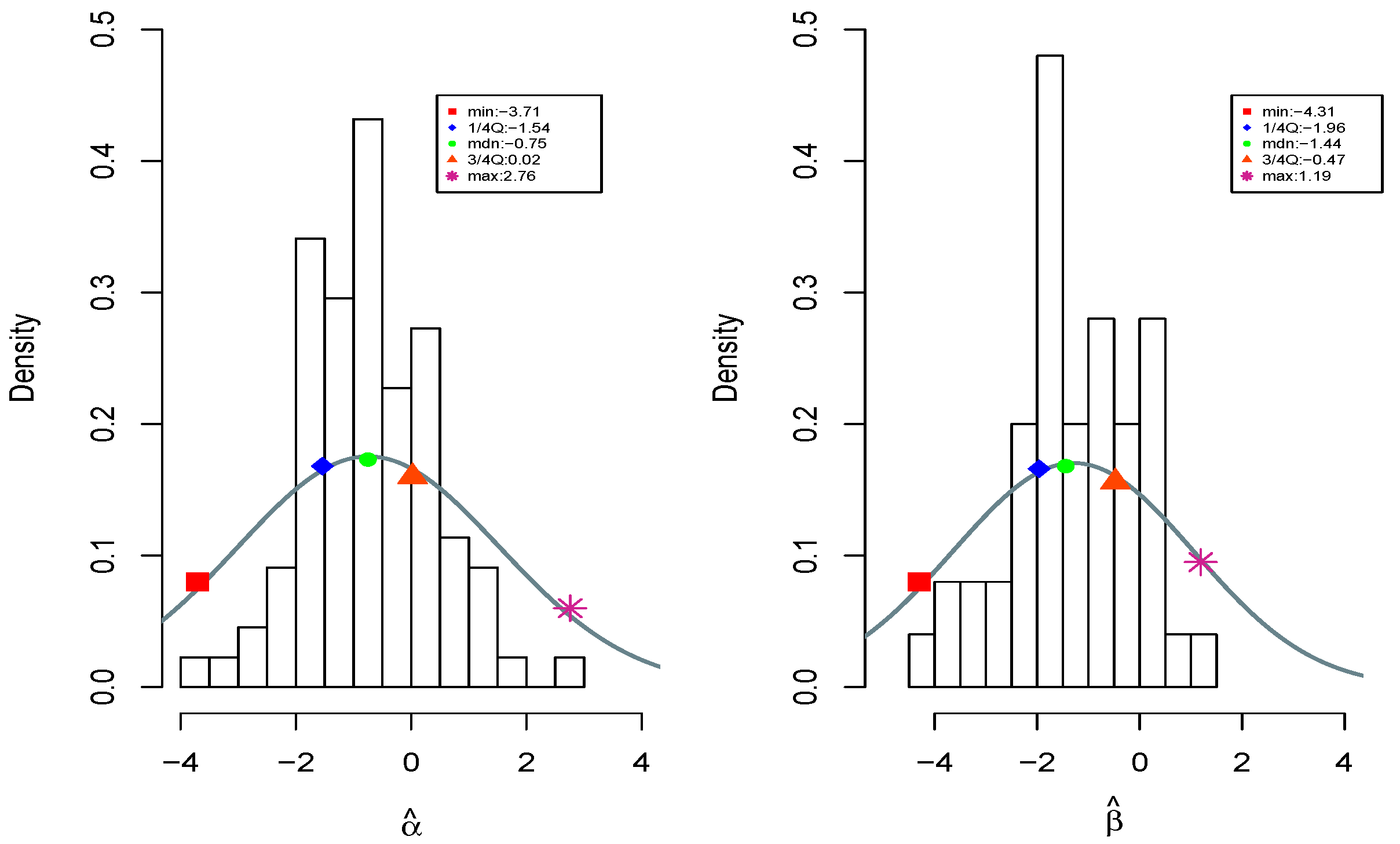
78	1	−3.71 (1.14)	36	1	−4.31 (0.99)

presents the estimators for users (${\widehat{\alpha }}_i$) and movies (${\widehat{\beta }}_j$), along with their standard errors, ranked by their degree sequences. Notably, we set ${\widehat{\beta }}_{50}=0$. Table 5 exhibits a positive correlation between $\widehat{\mathit{\alpha }}$ and $\mathbf{d}$, and likewise between $\widehat{\mathit{\beta }}$ and $\mathbf{b}$. For instance, User ID 1 with a degree of 78 has ${\widehat{\alpha }}_1$ of 2.76, whereas User ID 78 with a degree of 1 has −3.71. In the case of movies, Movie ID 7 with a degree of 101 has ${\widehat{\beta }}_7$ of 1.19, and Movie ID 36 with a degree of 1 has −4.31.

Table 6. The minimum, quartiles and maximum values of degrees from 88 users and 50 movies.

Degree	Minimum	$1/4$ Quantile	Median	$3/4$ Quantile	Maximum
d	1	7	12	21.5	78
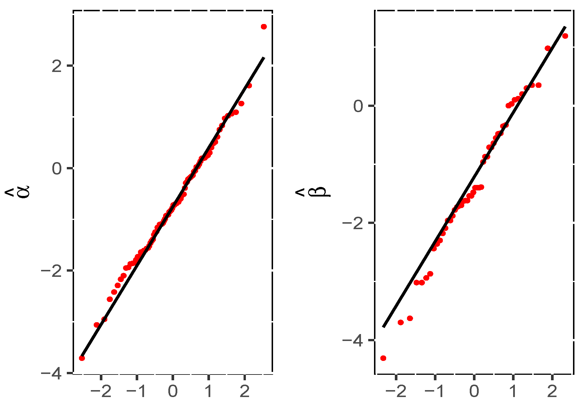
b	1	11	14.5	36.5	125

presents the quantiles of user- and movie-degrees, highlighting the wide range of values for $\mathbf{d}$ (from 1 to 78) and $\mathbf{b}$ (from 1 to 125). This variability is also reflected in the values of ${\widehat{\alpha }}_i$ and ${\widehat{\beta }}_j$, which range from −3.71 to 2.76 and −4.31 to 1.19, respectively, as shown in Figure 3. The histograms of both ${\widehat{\alpha }}_i$ and ${\widehat{\beta }}_j$ suggest approximate normal distributions. The Q-Q plots in Figure 4 compare the empirical and theoretical quantiles for ${\widehat{\alpha }}_i$ and ${\widehat{\beta }}_j$, with the red reference line representing $y=x$. In these plots, many points cluster near the reference line in the central region, indicating a good fit to the normal distribution for most estimators. In contrast, the greater variability of points in the tails suggests potential deviations from normality for extreme values. Overall, both ${\widehat{\alpha }}_i$ and ${\widehat{\beta }}_j$ approximate normal distributions.

As an application of our methodology, we generated 100 bootstrapped adjacency matrices using the estimated parameters. These matrices were then used to construct $95\%$ bootstrap confidence intervals for the degree sequences, as shown in

Table 7. MovieLens 100K Dataset: Mean degrees of 100 bootstrap degree sequences with $95\%$ bootstrap confidence intervals (CI) in square brackets, and listed top 10 and bottom 10 users and movies.

User ID	d	$\overline{\mathit{d}}$	$95\%$ Bootstrap CI	Movie ID	b	$\overline{\mathit{b}}$	$95\%$ Bootstrap CI
1	78	78.08	(71.10, 85.06)	1	89	86.84	(74.44, 99.24)
2	12	10.31	(4.84, 15.78)	2	16	15.13	(8.36, 21.90)
4	4	3.15	(−0.11, 6.41)	3	13	12.71	(5.71, 19.71)
5	17	15.59	(8.24, 22.94)	4	35	34.35	(22.79, 45.91)
6	25	23.45	(15.56,31.34)	5	12	11.73	(5.51, 17.95)
7	34	31.61	(22.26, 40.96)	6	14	13.41	(6.35, 20.47)
8	6	5.09	(1.05, 9.13)	7	101	99.76	(87.72, 111.80)
9	6	5.09	(0.47, 9.71)	8	51	49.96	(37.86, 62.06)
10	29	27.24	(19.37, 35.11)	9	69	68.20	(56.79, 79.61)
11	21	19.70	(11.41, 27.99)	10	17	16.16	(8.17, 24.15)
⋮	⋮	⋮	⋮	⋮	⋮	⋮	⋮
90	37	35.35	(25.37, 45.33)	41	4	3.77	(−0.10, 7.64)
91	8	7.00	(1.54, 12.46)	42	35	34.70	(25.08, 44.32)
92	44	43.03	(34.08, 51.98)	43	7	6.60	(1.11, 12.09)
93	6	4.96	(0.53, 9.39)	44	11	10.81	(4.53, 17.09)
94	44	43.65	(33.12, 54.18)	45	17	17.19	(10.48, 23.90)
95	29	26.93	(18.78, 35.08)	46	4	4.17	(0.39, 7.95)
96	11	9.91	(3.84, 15.98)	47	25	24.64	(14.23, 35.05)
97	12	10.79	(5.02, 16.56)	48	29	29.24	(19.44, 39.04)
98	4	3.64	(−0.13, 7.41)	49	14	13.53	(6.42, 20.64)
99	17	15.75	(8.57, 22.93)	50	125	43.25	(33.09, 53.41)

. Key insights from Table 7 reveal that the mean bootstrap degrees consistently approximate the observed degrees, confirming the accuracy of the bootstrap process. Notably, the original degrees almost always fall within their respective $95\%$ confidence intervals. This robust alignment highlights the reliability of the bootstrap method in replicating and understanding the degree distributions in large-scale network data, such as that of the MovieLens 100K Dataset. Additionally, the analysis in

Table 8. The skewness of degree distributions for 88 users and 50 movies: ${\beta }_S$ is the skewness of the original degree distributions. ${\widehat{\beta }}_{S_m}$ is the mean skewness from 100 bootstrap samples, and ${\widehat{\beta }}_{S_i}$ indicates skewness of the ith bootstrap sample.

Type	${\mathit{\beta }}_{\mathit{S}}$	${\widehat{\mathit{\beta }}}_{{\mathit{S}}_{\mathit{m}}}$	${\widehat{\mathit{\beta }}}_{{\mathit{S}}_1}$	${\widehat{\mathit{\beta }}}_{{\mathit{S}}_{25}}$	${\widehat{\mathit{\beta }}}_{{\mathit{S}}_{50}}$	${\widehat{\mathit{\beta }}}_{{\mathit{S}}_{75}}$	${\widehat{\mathit{\beta }}}_{{\mathit{S}}_{100}}$
Users	1.86	1.98	1.85	1.48	2.13	2.06	1.56
Movies	1.56	1.25	1.23	1.22	1.32	1.15	1.17

shows that the skewness of degree distributions across the bootstrap samples consistently aligns with the original distributions. For users, the mean bootstrap skewness ${\widehat{\beta }}_{S_m}$ is slightly higher, suggesting a minor variation among the samples. The skewness for movies is more consistent, as indicated by smaller deviations in the bootstrap samples. These patterns emphasize the robustness of the bootstrap method in reproducing the skewness characteristics of the original data.

Beyond the movie rating data, the GLAN model is suitable for various affiliation networks. It handles diverse node attributes, varying actor activities, and event popularity, making it suitable for social networks, e-commerce, and academic collaborations. For example, in social networks, the GLAN model analyzes user-post interactions, where users have varying activity levels (e.g., posting frequency) and posts have varying popularity (e.g., likes, shares). In e-commerce, the GLAN model examines how users interact with products, with product popularity shaped by user preferences and behavior.

6. Discussion

In this paper, we introduce a novel approach to modeling affiliation networks using the GLAN model (1). This model effectively incorporates node attributes by considering actor activeness, event popularity, and additional interaction factors. By rigorously applying MLE, we navigate the complexities of network structures. We demonstrate that, under appropriate conditions, the MLEs for degree heterogeneity and node homophily parameters converge to multivariate normal distributions. The model’s effectiveness and robustness are illustrated through simulations and empirical studies using the MovieLens 100K dataset. These results provide practical validation of the model’s ability to capture and analyze affiliation networks, which differ from the one-mode networks typically studied in previous research.

Several interesting directions remain for future work. For instance, incorporating temporal dynamics into the GLAN model (1) could allow it to capture the evolution of networks over time, offering a more dynamic and comprehensive understanding of network changes. Additionally, developing scalable algorithms is crucial for extending the model’s applicability to larger datasets, thus enhancing its practical value across various contexts.

Another promising area for exploration is the effect of differing growth rates between network size and node attribute dimensions. Significant variations in these growth rates could notably impact the convergence properties of the estimators. This fundamental aspect of our theoretical framework would influence subsequent derivations and conclusions, while we consider this to be a feasible direction for future research, it falls outside the scope of this paper.

References

1. Newman, M.E. The structure and function of complex networks. SIAM Rev. 2003, 45, 167–256. [Google Scholar] [CrossRef]
2. Myall, A.; Peach, R.; Wan, Y.; Mookerjee, S.; Jauneikaite, E.; Bolt, F.; Price, J.; Davies, F.; Weisse, A.; Holmes, A.; et al. Improved contact tracing using network analysis and spatial-temporal proximity. Int. J. Infect. Dis. 2022, 116, S20. [Google Scholar] [CrossRef]
3. Ke, Z.; Vikalo, H. Graph-based reconstruction and analysis of disease transmission networks using viral genomic data. J. Comput. Biol. 2023, 30, 796–813. [Google Scholar] [CrossRef]
4. Boone, C.; Bussey, H.; Andrews, B.J. Exploring genetic interactions and networks with yeast. Nat. Rev. Genet. 2007, 8, 437–449. [Google Scholar] [CrossRef] [PubMed]
5. Mair, B.; Moffat, J.; Boone, C.; Andrews, B.J. Genetic interaction networks in cancer cells. Curr. Opin. Genet. Dev. 2019, 54, 64–72. [Google Scholar] [CrossRef]
6. Guillaume, J.L.; Latapy, M. Bipartite graphs as models of complex networks. Phys. Stat. Mech. Its Appl. 2006, 371, 795–813. [Google Scholar] [CrossRef]
7. Pavlopoulos, G.A.; Kontou, P.I.; Pavlopoulou, A.; Bouyioukos, C.; Markou, E.; Bagos, P.G. Bipartite graphs in systems biology and medicine: A survey of methods and applications. GigaScience 2018, 7, giy014. [Google Scholar] [CrossRef]
8. Zhou, C.; Feng, L.; Zhao, Q. A novel community detection method in bipartite networks. Phys. Stat. Mech. Its Appl. 2018, 492, 1679–1693. [Google Scholar] [CrossRef]
9. Frank, O.; Strauss, D. Markov graphs. J. Am. Stat. Assoc. 1986, 81, 832–842. [Google Scholar] [CrossRef]
10. Park, J.; Newman, M.E. Statistical mechanics of networks. Phys. Rev. E 2004, 70, 066117. [Google Scholar] [CrossRef]
11. Lusher, D.; Koskinen, J.; Robins, G. Exponential Random Graph Models for Social Networks: Theory, Methods, and Applications; Cambridge University Press: Cambridge, UK, 2013. [Google Scholar]
12. Cimini, G.; Squartini, T.; Saracco, F.; Garlaschelli, D.; Gabrielli, A.; Caldarelli, G. The statistical physics of real-world networks. Nat. Rev. Phys. 2019, 1, 58–71. [Google Scholar] [CrossRef]
13. Hillar, C.; Wibisono, A. Maximum entropy distributions on graphs. arXiv 2013, arXiv:1301.3321. [Google Scholar]
14. Chen, M.; Kato, K.; Leng, C. Analysis of networks via the sparse β-model. J. R. Stat. Soc. Ser. Stat. Methodol. 2021, 83, 887–910. [Google Scholar] [CrossRef]
15. Du, Y.; Qu, L.; Yan, T.; Zhang, Y. Time-varying β-model for dynamic directed networks. Scand. J. Stat. 2023, 50, 1687–1715. [Google Scholar] [CrossRef]
16. Yan, T.; Li, Y.; Xu, J.; Yang, Y.; Zhu, J. Likelihood ratio tests in random graph models with increasing dimensions. arXiv 2023, arXiv:2311.05806. [Google Scholar] [CrossRef]
17. Shao, M.; Zhang, Y.; Wang, Q.; Zhang, Y.; Luo, J.; Yan, T. L2 Regularized maximum likelihood for β-model in large and sparse networks. arXiv 2021, arXiv:2110.11856. [Google Scholar]
18. Yan, T.; Xu, J. A central limit theorem in the β-model for undirected random graphs with a diverging number of vertices. Biometrika 2013, 100, 519–524. [Google Scholar] [CrossRef]
19. Yan, T.; Leng, C.; Zhu, J. Asymptotics in directed exponential random graph models with an increasing bi-degree sequence. Ann. Stat. 2016, 44, 31–57. [Google Scholar] [CrossRef]
20. Yan, T.; Qin, H.; Wang, H. Asymptotics in undirected random graph models parameterized by the strengths of vertices. Stat. Sin. 2016, 26, 273–293. [Google Scholar] [CrossRef]
21. Fan, Y.; Zhang, H.; Yan, T. Asymptotic Theory for Differentially Private Generalized β-models with Parameters Increasing. Stat. Interface 2020, 13, 385–398. [Google Scholar] [CrossRef]
22. Zhang, Y.; Qian, X.; Qin, H.; Yan, T. Affiliation networks with an increasing degree sequence. Commun. Stat. Theory Methods 2017, 46, 11163–11180. [Google Scholar] [CrossRef][Green Version]
23. Fan, Y.; Jiang, B.; Yan, T.; Zhang, Y. Asymptotic theory in bipartite graph models with a growing number of parameters. Can. J. Stat. 2023, 51, 919–942. [Google Scholar] [CrossRef]
24. Wang, Q.; Yan, T.; Jiang, B.; Leng, C. Two-mode networks: Inference with as many parameters as actors and differential privacy. J. Mach. Learn. Res. 2022, 23, 1–38. [Google Scholar]
25. Luo, J.; Liu, T.; Wang, Q. Affiliation weighted networks with a differentially private degree sequence. Stat. Pap. 2022, 63, 367–395. [Google Scholar] [CrossRef]
26. Pan, L.; Hu, J. Differentially private estimation in a class of bipartite graph models. Commun. Stat. Theory Methods 2024, 53, 6477–6496. [Google Scholar] [CrossRef]
27. Sarkar, P.; Siddiqi, S.M.; Gordon, G.J. A latent space approach to dynamic embedding of co-occurrence data. In Proceedings of the Eleventh International Conference on Artificial Intelligence and Statistics, San Juan, Puerto Rico, 21–24 March 2007; pp. 420–427. [Google Scholar]
28. Friel, N.; Rastelli, R.; Wyse, J.; Raftery, A.E. Interlocking directorates in Irish companies using a latent space model for bipartite networks. Proc. Natl. Acad. Sci. USA 2016, 113, 6629–6634. [Google Scholar] [CrossRef] [PubMed]
29. Zhang, Y.; Pan, R.; Wang, F.; Fang, K.; Wang, H. Network embedding for bipartite networks with applications in interlocking directorates in Chinese companies. Comput. Stat. 2025, 40, 1–36. [Google Scholar] [CrossRef]
30. Razaee, Z.S.; Amini, A.A.; Li, J.J. Matched bipartite block model with covariates. J. Mach. Learn. Res. 2019, 20, 1–44. [Google Scholar]
31. Wu, Y.; Lan, W.; Fan, X.; Fang, K. Bipartite network influence analysis of a two-mode network. J. Econom. 2024, 239, 105562. [Google Scholar] [CrossRef]
32. Qing, H.; Wang, J. Bipartite mixed membership stochastic blockmodel. stat 2021, 1050, 7. [Google Scholar]
33. Graham, B.S. An econometric model of network formation with degree heterogeneity. Econometrica 2017, 85, 1033–1063. [Google Scholar] [CrossRef]
34. Yan, T.; Jiang, B.; Fienberg, S.E.; Leng, C. Statistical inference in a directed network model with covariates. J. Am. Stat. Assoc. 2019, 114, 857–868. [Google Scholar] [CrossRef]
35. Wang, Q.; Zhang, Y.; Yan, T. Asymptotic theory in network models with covariates and a growing number of node parameters. Ann. Inst. Stat. Math. 2023, 75, 369–392. [Google Scholar] [CrossRef]
36. Huang, S.; Sun, J.; Feng, Y. PCABM: Pairwise covariates-adjusted block model for community detection. J. Am. Stat. Assoc. 2024, 119, 2092–2104. [Google Scholar] [CrossRef]
37. Harper, F.M.; Konstan, J.A. The MovieLens Datasets: History and Context. ACM Trans. Interact. Intell. Syst. 2015, 5, 1–19. [Google Scholar] [CrossRef]
38. Fernandez, J.A.E.; Verón, M.Á.H. Mild Differentiability Conditions for Newton’s Method in Banach Spaces; Springer Nature: Berlin, Germany, 2020. [Google Scholar]
39. Chatterjee, S.; Diaconis, P.; Sly, A. Random graphs with a given degree sequence. Ann. Appl. Probab. 2011, 21, 1400–1435. [Google Scholar] [CrossRef]
40. Loéve, M. Probability Theory I, 4th ed.; Springer: New York, NY, USA, 1977. [Google Scholar]
41. Dzemski, A. An Empirical Model of Dyadic Link Formation in a Network with Unobserved Heterogeneity. Rev. Econ. Stat. 2019, 101, 763–776. [Google Scholar] [CrossRef]
Figure 1. Visualization of Movie Rating Network: Top 10 % User Nodes & Top 20 % Movie Nodes.
Symmetry 17 02005 g001
Figure 2. The QQ plots of v ^ i , i 1 / 2 ( α ^ i α i ) for ( m , n ) = ( 100 , 50 ) .
Symmetry 17 02005 g002
Figure 3. Histograms of α ^ i ’s and β ^ j ’s for 88 Users and 50 Movies in the MovieLens 100K Dataset.
Symmetry 17 02005 g003
Figure 4. The QQ plots of α ^ i ’s and β ^ j ’s for 88 Users (left) and 50 Movies (right) in the MovieLens 100K Dataset.
Symmetry 17 02005 g004