Two Novel Sparse Models for Support Vector Machines

Abstract

Based on the Support Vector Machine (SVM) and Twin Parametric Margin SVM (TPMSVM), this paper proposes two sparse models, named Sparse SVM (SSVM) and Sparse TPMSVM (STPMSVM). The study aims to achieve high sparsity, rapid prediction, and strong generalization capability by transforming the classical quadratic programming problems (QPPs) into linear programming problems (LPPs). The core idea stems from a clear geometric motivation: introducing an ${\ell }_1$-norm penalty on the dual variables to break the inherent rotational symmetry of the traditional ${\ell }_2$-norm on the normal vector. Through a theoretical reformulation using the Karush–Kuhn–Tucker (KKT) conditions, we achieve a transformation from explicit symmetry-breaking to implicit structural constraints—the ${\ell }_1$ penalty term does not appear explicitly in the final objective function, while the sparsity-inducing effect is fundamentally encoded within the objective functions and their constraints. Ultimately, the derived linear programming models naturally yield highly sparse solutions. Extensive experiments are conducted on multiple synthetic datasets under various noise conditions, as well as on 20 publicly available benchmark datasets. Results demonstrate that the two sparse models achieve significant sparsity at the support vectors level—on the benchmark datasets, SSVM, and STPMSVM reduce the number of support vectors by an average of 56.21% compared with conventional SVM, while STPMSVM achieves an average reduction of 39.11% compared with TPMSVM—thereby greatly improving prediction efficiency. Notably, SSVM maintains accuracy comparable to conventional SVM under low-noise conditions while attaining extreme sparsity and prediction efficiency. In contrast, STPMSVM offers enhanced robustness to noise and maintains a better balance between sparsity and accuracy, preserving the desirable properties of TPMSVM while improving prediction efficiency and robustness.

1. Introduction

Machine learning methods are popular and extremely efficient for solving classification and regression problems [1], attracting the attention of many researchers. Various algorithms for supervised and unsupervised learning have been proposed and extensively studied in the past few decades. Among them, Support Vector Machine (SVM) [1,2,3,4,5] and its variants [6,7,8,9,10] are widely recognized as some of the most powerful supervised learning algorithms based on kernel techniques. SVM was first proposed by Cortes and Vapnik [2] for classification and later extended to regression problems. It maps the samples into a higher-dimensional feature space and generates a pair of parallel optimal linear separating hyperplanes with maximal margin. Due to its extraordinary generalization capability, discriminative power, and strong theoretical properties [2,3,4,5], SVM has been widely applied in diverse research fields [6,11,12,13,14,15,16,17,18,19].

In recent years, several enhanced SVM formulations have been developed to improve flexibility and predictive performance. To increase the predictive power of SVM, par-v-SVM [7] was proposed, introducing a flexible parametric margin, where the parameter can control the number of support vectors and margin errors. Khemchandani et al. [8] proposed Twin SVM (TWSVM) for binary datasets. Instead of determining two parallel hyperplanes as in traditional SVM, TWSVM determines one hyperplane for each class, ensuring each hyperplane is as close as possible to one of the two classes and as far as possible from the other. This approach requires solving two lower-dimensional quadratic programming problems (QPPs) instead of one large optimization problem in the classical SVM method, making TWSVM almost four times faster than the standard SVM classifier. In 2011, combining TWSVM and par-v-SVM, a novel Twin Parametric Margin SVM (TPMSVM) [9] was proposed, where again two nonparallel parametric-margin separating hyperplanes are generated. Like TWSVM, TPMSVM also solves two QPPs but introduces adaptive margins to enhance flexibility, drawing inspiration from par-v-SVM. It has also been extended to improve robustness and handle multiclass problems [20].

With the growing demand for efficient machine learning in resource-constrained environments such as edge computing, achieving sparsity in SVMs has become increasingly important. Reducing the number of support vectors can lower memory and computational requirements while accelerating prediction without compromising generalization performance. Several approaches have been explored to induce sparsity in SVMs: Some methods introduce non-convex loss functions [19,21,22] or non-convex regularization terms [23,24,25,26] to promote sparsity, but these typically require complex optimization algorithms; Another line of work imposes sparsity constraints on SVMs to directly control the number of support vectors [27,28], achieving effective sparsity, but both involve theoretically intricate frameworks and rely on iterative optimization procedures, which reduces their simplicity and scalability. Meanwhile, classical ${\ell }_1$ regularization [29] primarily induces sparsity at the feature level, while support vector sparsity still largely stems from the natural sparsity of the hinge loss.

Motivated by these limitations, we propose sparse SVM (SSVM) and sparse TPMSVM (STPMSVM) based on our previous work [30,31]. Both models directly impose an ${\ell }_1$ penalty on the dual variables to induce sparsity at the support vector level. By reformulating the original QPPs via the Karush–Kuhn–Tucker (KKT) conditions, we achieve a key novelty of our work: their structural transformation into convex linear programming problems (LPPs). Critically, while the classical ${\ell }_1$-norm SVM also yields an LPP, its objective involves a non-smooth ${\ell }_1$-norm. In contrast, our reformulation results in a standard LPP with an inherently linear objective, which presents a more compact structure for the solver and thereby enables efficient solution, ensures principled sparsity, and significantly improves prediction efficiency—all without compromising generalization performance. Table 1 further summarizes the main conceptual differences between the classical ${\ell }_1$-norm SVM and the proposed sparse models in this paper, highlighting dual-level sparsity and LPP reformulation.

Table 1. Conceptual comparison of classical ${\ell }_1$-norm SVM and proposed sparse models.

Model	Variable Penalized	Sparsity Level	Optimization
${\ell }_1$-norm SVM	Weight vector	Feature level	Single LPP with a ${\parallel ·\parallel }_1$ objective
SSVM	Dual variable	Support vector level	Single LPP with a standard linear objective
STPMSVM	Dual variables	Support vector level	Two LPPs with standard linear objectives

The main contributions of this paper are summarized as follows:

• Two Novel Sparse Models: We propose two novel sparse models: Sparse SVM (SSVM) and Sparse TPMSVM (STPMSVM), with sparsity as a central design objective.
• Symmetry-Driven Sparsification: Sparsity is induced by breaking the rotational symmetry of the ${\ell }_2$-norm through an ${\ell }_1$ penalty on the dual variables, a geometric motivation that is then implicitly encoded into the model structure via the KKT conditions.
• Novel KKT-based reformulations transform the traditional QPPs into corresponding LPPs for both models.
• Significant Prediction Efficiency: The LPPs, combined with induced sparsity at the support vector level, allow faster prediction compared with the traditional QPP-based methods.
• Extensive Experimental Validation: Comprehensive experiments on synthetic and benchmark datasets verify that the proposed models achieve an advantageous trade-off among sparsity, prediction speed, and generalization performance.

The remainder of this paper is organized as follows. Section 2 briefly describes the fundamentals of the classical SVM and TPMSVM models. Section 3 then introduces the proposed SSVM and STPMSVM models, accompanied by theoretical analysis and discussion. Extensive numerical experiments are conducted in Section 4 using multiple synthetic datasets and 20 publicly available benchmark datasets. Finally, the conclusions and further work are presented in Section 5.

2. Fundamentals of SVM and TPMSVM Models

Since most of the practical problems are nonlinear in nature, in this paper we mainly discuss the nonlinear classification case. We will review the classical SVM model and TPMSVM model in this section. First, we briefly describe some notations used in this paper.

2.1. Notations

The set of real numbers will be denoted by $\mathbb{R}$. All vectors are column vectors and will be denoted with lowercase Latin letters. The space of the $P\times n$ matrices with real components will be indicated by ${\mathbb{R}}^{P\times n}$. Matrices will be indicated with uppercase Roman letters.

We assume that the training set

$$\{(x^p,y_p),p=1,2,\dots ,P,x^p\in {\mathbb{R}}^n,y_p\in \{-1,1\}\}$$

is given. Other notations are listed in Table 2.

Table 2. List of notations.

Notation	Description
$\left|I\right|$	The number of elements in a index set I
$I_{\pm }$	The index set of positive/negative samples, $I_{+}\bigcap I_{-}=\Phi ,I_{+}\bigcup I_{-}=\{1,2,\dots ,P\},|I_{+}|+|I_{-}|=P$
n	The dimension of samples
$X_{+}$	$X_{+}={[X_{+}=x^1,\dots ,x^i,\dots ,x^{|I_{+}|}]}^T\in {\mathbb{R}}^{|I_{+}|\times n},i\in I_{+}$, the positive samples matrix for the TPMSVM and STPMSVM models
$X_{-}$	$X_{-}={[x^{|I_{+}|+1},\dots ,x^{|I_{+}|+k},\dots ,x^P]}^T\in {\mathbb{R}}^{|I_{-}|\times n},k=1,2,\dots ,\left|I_{-}\right|$, the negative samples matrix for the TPMSVM and STPMSVM models
e	The vector of opportune dimensions with all components equal to 1
$\phi (·)$	The mapping function from the original input space to the feature space
$\phi \left(X_{+}\right)$	$\phi \left(X_{+}\right)=[\phi \left(x^1\right),\dots ,\phi \left(x^i\right),\dots ,\phi {\left(x^{|I_{+}|}\right]}^T\in {\mathbb{R}}^{|I_{+}|\times n},i\in I_{+}$, the positive samples mapping matrix for the TPMSVM and STPMSVM models
$\phi \left(X_{-}\right)$	$\phi \left(X_{-}\right)={[\phi \left(x^{|I_{+}|+1}\right),\dots ,\phi \left(x^{|I_{+}|+k}\right),\dots ,\phi \left(x^P\right)]}^T\in {\mathbb{R}}^{|I_{-}|\times n},k=1,2,\dots ,\left|I_{-}\right|$, the negative samples mapping matrix for the TPMSVM and STPMSVM models
$⟨·,·⟩$	The inner product of two vectors

2.2. SVM Model

The primal problem for the classical SVM for the nonlinear case (for the linear cases, the kernel function $\phi (·)$ is just the identity function) is as follows:

$$\begin{array}{cc}\hfill \underset{w,\theta ,\xi }{min}& {\displaystyle \frac{1}{2}}{\parallel w\parallel }_2^2+\rho e^T\xi \hfill \\ \hfill \mathrm{subject}\mathrm{to}& y_p(⟨w,\phi \left(x^p\right)⟩+\theta )\ge 1-{\xi }_p,{\xi }_p\ge 0,p=1,\dots ,P,\hfill \end{array}$$

(1)

where $\rho$ is the regularization factor and $\xi ={[{\xi }_1,{\xi }_2,\dots ,{\xi }_P]}^T\in {\mathbb{R}}^P$ is the slack vector. The Wolfe dual problem [32] of (1) is as follows:

$$\begin{array}{cc}\hfill \underset{\alpha }{min}& {\displaystyle \frac{1}{2}}{\alpha }^{T}Q\alpha -e^T\alpha \hfill \\ \hfill \mathrm{subject}\mathrm{to}& y^T\alpha =0,0\le \alpha \le \rho e,\hfill \end{array}$$

(2)

where $\alpha ={[{\alpha }_1,{\alpha }_2,\dots ,{\alpha }_P]}^T\in {\mathbb{R}}^P$ is the dual variable, $Q\in {\mathbb{R}}^{P\times P},Q_{pq}=y_p{y}_{q}K(x^p,x^q)$, $p,q\in \{1,2,\dots ,P\}$, and $K(x^p,x^q)=⟨\phi \left(x^p\right),\phi \left(x^q\right)⟩$ is the kernel function. From the KKT conditions, we also obtain the following:

$$\begin{array}{c}\hfill {\displaystyle w=\sum _{p=1}^P{\alpha }^p{y}_p\phi \left(x^p\right).}\end{array}$$

(3)

This expression connects the normal vector w with the dual variables $\alpha$, which will be fundamental in deriving our SSVM models in the subsequent sections. After solving the dual problem (2), the vector w can be obtained from (3) and the bias term:

$$\begin{array}{c}\hfill \theta =-{\displaystyle \frac{1}{\left|N\right|}}\sum _{p\in N}{y}_p-w^T\phi \left(x^p\right)\end{array}$$

(4)

can be calculated, where N is the index set of the training samples satisfying $0<{\alpha }_p<\rho ,p=1,\dots ,P$. Finally, the decision hyperplane is given by the following:

$$\begin{array}{c}\hfill f\left(x\right)=w^T\phi \left(x\right)+\theta =0.\end{array}$$

(5)

The two margin hyperplanes are $f\left(x\right)+1=0$ and $f\left(x\right)-1=0$, respectively. Geometrically, these two margins are symmetric with respect to the decision hyperplane. A new sample x can be assigned to the class +1 or–1 according to the sign of the decision function $f\left(x\right)$ in (5).

Note that the prediction efficiency of SVM, as indicated by its decision function (5), depends critically on the number of the support vectors in (3). Although the standard SVM naturally acquires some sparsity through the hinge loss, it does not actively enforce it.

2.3. TPMSVM Model

For the TPMSVM model, the following two symmetric hyperplanes in the feature space are considered as follows:

$$\begin{array}{c}\hfill f_1\left(x\right)={w^{+}}^T\phi \left(x\right)+{\theta }_{+}=0,f_2\left(x\right)={w^{-}}^T\phi \left(x\right)+{\theta }_{-}=0.\end{array}$$

(6)

The TPMSVM is then formulated as a pair of symmetric QPPs, whose primal problems are as follows:

$$\begin{array}{cc}\hfill \underset{w^{+},{\theta }_{+},{\xi }^{+}}{min}& {\displaystyle \frac{1}{2}}{\parallel w^{+}\parallel }_2^2+{\displaystyle \frac{v_{+}}{|I_{-}|}}{e}^T(\phi \left(X_{-}\right)w^{+}+e{\theta }_{+})+{\displaystyle \frac{{\rho }_{+}}{|I_{+}|}}{e}^T{\xi }^{+}\hfill \\ \hfill \mathrm{subject}\mathrm{to}& \phi \left(X_{+}\right)w^{+}+{\theta }_{+}e\ge -{\xi }^{+},{\xi }^{+}\ge 0,\hfill \end{array}$$

(7)

$$\begin{array}{cc}\hfill \underset{w^{-},{\theta }_{-},{\xi }^{-}}{min}& {\displaystyle \frac{1}{2}}{\parallel w^{-}\parallel }_2^2-{\displaystyle \frac{v_{-}}{|I_{+}|}}{e}^T(\phi \left(X_{+}\right)w^{-}+e{\theta }_{-})+{\displaystyle \frac{{\rho }_{-}}{|I_{-}|}}{e}^T{\xi }^{-}\hfill \\ \hfill \mathrm{subject}\mathrm{to}& \phi \left(X_{-}\right)w^{-}+{\theta }_{-}e\le {\xi }^{-},{\xi }^{-}\ge 0,\hfill \end{array}$$

(8)

where $v_{+},v_{-},{\rho }_{+}$ and ${\rho }_{-}$ are regularization parameters, ${\xi }^{+}\in {\mathbb{R}}^{|I_{+}|}$ and ${\xi }^{-}\in {\mathbb{R}}^{|I_{-}|}$ are slack vectors. Next, we introduce the following notations for convenience:

$$\begin{array}{cc}\hfill K^{++}=\phi \left(X_{+}\right){\phi \left(X_{+}\right)}^T\in {\mathbb{R}}^{|I_{+}|\times |I_{+}|}:& K_{pq}^{++}=⟨\phi \left(x^p\right),\phi \left(x^q\right)⟩,p,q\in I_{+}\hfill \\ \hfill K^{+-}=\phi \left(X_{+}\right){\phi \left(X_{-}\right)}^T\in {\mathbb{R}}^{|I_{+}|\times |I_{-}|}:& K_{pq}^{+-}=⟨\phi \left(x^p\right),\phi \left(x^q\right)⟩,p\in I_{+},q\in I_{-}\hfill \\ \hfill K^{-+}=\phi \left(X_{-}\right){\phi \left(X_{+}\right)}^T\in {\mathbb{R}}^{|I_{-}|\times |I_{+}|}:& K_{pq}^{-+}=⟨\phi \left(x^p\right),\phi \left(x^q\right)⟩,p\in I_{-},q\in I_{+}\hfill \\ \hfill K^{--}=\phi \left(X_{-}\right){\phi \left(X_{-}\right)}^T\in {\mathbb{R}}^{|I_{-}|\times |I_{-}|}:& K_{pq}^{--}=⟨\phi \left(x^p\right),\phi \left(x^q\right)⟩,p,q\in I_{-}\hfill \end{array}$$

(9)

Obviously, $K^{++}$ and $K^{--}$ are symmetric matrices and ${\left(K^{+-}\right)}^T=K^{-+}$. By introducing the Lagrangian function for (7) and (8), respectively, and from the KKT conditions, we obtain the following:

$$\begin{array}{c}\hfill w^{+}=\phi {\left(X_{+}\right)}^T{\alpha }^{+}-{\displaystyle \frac{v_{+}}{|I_{-}|}}\phi {\left(X_{-}\right)}^{T}e,\end{array}$$

(10)

$$\begin{array}{c}\hfill e^T{\alpha }^{+}=v_{+},0\le {\alpha }^{+}\le {\displaystyle \frac{{\rho }_{+}}{|I_{+}|}}e\end{array}$$

(11)

and

$$\begin{array}{c}\hfill w^{-}=-\phi {\left(X_{-}\right)}^T{\alpha }^{-}+{\displaystyle \frac{v_{-}}{|I_{+}|}}\phi {\left(X_{+}\right)}^{T}e.\end{array}$$

(12)

$$\begin{array}{c}\hfill e^T{\alpha }^{-}=v_{-},0\le {\alpha }^{-}\le {\displaystyle \frac{{\rho }_{-}}{|I_{-}|}}e.\end{array}$$

(13)

where ${\alpha }^{+}=[{\alpha }_1^{+},{\alpha }_2^{+},\dots ,{\alpha }_{|I_{+}|}^{+}]\in {\mathbb{R}}^{|I_{+}|}$ and ${\alpha }^{-}=[{\alpha }_1^{-},{\alpha }_2^{-},\dots ,{\alpha }_{|I_{-}|}^{-}]\in {\mathbb{R}}^{|I_{-}|}$ are the dual variables. Similar to the classical SVM, the hyperplane normal vector $w^{+}$ is expressed in terms of the dual variables ${\alpha }^{+}$ and the samples from the negative class; a corresponding expression for $w^{-}$ involves ${\alpha }^{-}$ and the positive class samples. We especially point out that the expression of $w^{+}$ and $w^{-}$ in formulas (10) and (12) will be the important basis on which we later construct the STPMSVM model.

The Wolfe dual problems of (7) and (8) are, respectively, as follows:

$$\begin{array}{cc}\hfill \underset{{\alpha }^{+}}{min}& {\displaystyle \frac{1}{2}}{{\alpha }^{+}}^T{K}^{++}{\alpha }^{+}-{\displaystyle \frac{v_{+}}{|I_{-}|}}{e}^T{K}^{-+}{\alpha }^{+}\hfill \\ \hfill \mathrm{subject}\mathrm{to}& e^T{\alpha }^{+}=v_{+},0\le {\alpha }^{+}\le {\displaystyle \frac{{\rho }_{+}}{|I_{+}|}}e,\hfill \end{array}$$

(14)

and

$$\begin{array}{cc}\hfill \underset{{\alpha }^{-}}{min}& {\displaystyle \frac{1}{2}}{\alpha }^{-}{K}^{--}{\alpha }^{-}-{\displaystyle \frac{v_{-}}{|I_{+}|}}{e}^T{K}^{+-}{\alpha }^{-}\hfill \\ \hfill \mathrm{subject}\mathrm{to}& e^T{\alpha }^{-}=v_{-},0\le {\alpha }^{-}\le {\displaystyle \frac{{\rho }_{-}}{|I_{-}|}}e.\hfill \end{array}$$

(15)

After solving the symmetric dual problems (14) and (15), we can obtain $w^{+}$ and $w^{-}$ according to (10) and (12). In addition, the bias term ${\theta }_{\pm }$ can be computed as follows:

$$\begin{array}{c}\hfill {\theta }_{+}=-{\displaystyle \frac{1}{|N_{+}|}}\sum _{p\in N_{+}}{w^{+}}^T\phi \left(x^p\right),{\theta }_{-}=-{\displaystyle \frac{1}{|N_{-}|}}\sum _{q\in N_{-}}{w^{-}}^T\phi \left(x^q\right)\end{array}$$

(16)

where $N_{+}$ and $N_{-}$ are the index sets of positive and negative samples satisfying ${\alpha }_p^{+}\in (0,{\displaystyle \frac{{\rho }_{+}}{|I_{+}|}}),p\in N_{+}$ and ${\alpha }_q^{-}\in (0,{\displaystyle \frac{{\rho }_{-}}{|I_{-}|}}),q\in N_{-}$, respectively. The decision function of the TPMSVM can be constructed after solving the dual QPPs (14) and (15) as follows:

$$\begin{array}{c}\hfill f\left(x\right)=\mathrm{sign}[{({\widehat{w}}^{+}+{\widehat{w}}^{-})}^T\phi \left(x\right)+({\widehat{\theta }}_{+}+{\widehat{\theta }}_{-})],\end{array}$$

(17)

where ${\displaystyle {\widehat{w}}^{\pm }=\frac{w^{\pm }}{{∥w^{\pm }∥}_2},{\widehat{\theta }}_{\pm }=\frac{{\theta }_{\pm }}{{∥w^{\pm }∥}_2}}$. A new point x will be assigned to class +1 or −1 according to (17).

While TPMSVM introduces non-parallel hyperplanes for enhanced flexibility, its sparsity—Inherited naturally from the hinge loss similar to SVM—is limited due to the lack of an explicit sparsity mechanism. A more critical limitation arises from its decision function: unlike SVM, which relies solely on support vectors, the normal vector of TPMSVM (as shown in (10) and (12)) is determined by both its own support vectors and all samples from the other class. This inherent dependency, evident in the decision function (17), suggests that under comparable conditions, TPMSVM is theoretically less prediction-efficient than SVM.

2.4. Geometric Insight: ${\ell }_1$ vs. ${\ell }_2$ Regularization

The fundamental difference between ${\ell }_1$ and ${\ell }_2$ regularization can be illustrated through their geometry. The ${\ell }_2$-norm is rotationally symmetric; its spherical isosurfaces favor solutions where parameters are generally non-zero, leading to dense models. In contrast, the ${\ell }_1$-norm is not rotationally symmetric; its diamond-like (or cross-polytope) isosurfaces are aligned with the coordinate axes. This axis-aligned geometry inherently breaks the rotational symmetry and favors solutions that lie on the axes, where many parameters are exactly zero, thus inducing sparsity. This well-established geometric property provides the theoretical motivation for our approach. It suggests that imposing an ${\ell }_1$ penalty on the dual variables is expected to explicitly promote sparser solutions at the support vector level. Building on this insight, we develop two novel sparse models (SSVM and STPMSVM) by incorporating such a penalty into the SVM and TPMSVM frameworks, respectively, to actively induce sparsity while preserving their respective advantages.

3. Two Novel Sparse Models

In this section, we will describe the framework of our novel sparse models based on SVM and TPMSVM, respectively.

3.1. SSVM Model

To describe the SSVM model, we substitute (3) into the first constraint of the optimization problem (1) to obtain the following:

$$\begin{array}{c}\hfill y_p(⟨w,\phi \left(x^p\right)⟩+\theta )=\sum _{q=1}^P{\alpha }_q{y}_p{y}_{q}K(x^q,x^p)+y_p\theta \ge 1-{\xi }_p,p=1,2,\dots ,P.\end{array}$$

(18)

By replacing ${\displaystyle \frac{1}{2}}{\parallel w\parallel }_2^2$ in (1) with the ${\ell }_1$-norm of the dual variable $\alpha$, substituting the first constraint of (1) with (18), and incorporating the constraints from (2), we obtain the following:

$$\begin{array}{cc}\hfill \underset{\alpha ,\theta ,\xi }{min}& {\parallel \alpha \parallel }_1+\rho e^T\xi \hfill \\ \hfill \mathrm{subject}\mathrm{to}& \sum _{q=1}^P{\alpha }_q{y}_p{y}_{q}K(x^q,x^p)+y_p\theta \ge 1-{\xi }_p,{\xi }_p\ge 0,p=1,\dots ,P,\hfill \\ \hfill & y^T\alpha =0,0\le \alpha \le \rho e.\hfill \end{array}$$

(19)

The optimization problem (19) represents the embryonic form of the SSVM model. We point out that the first term of the objective function in (19) performs a global optimization over the dual variables, which inherently ensures a highly sparse solution, while the final two constraints originate from the KKT conditions. The remaining terms retain the same interpretation as in standard SVM, as they are obtained through the substitution described above.

Note that $\alpha \ge 0$ in (19), thus ${\parallel \alpha \parallel }_1$ can be expressed as $e^T\alpha$, then (19) can be rewritten as follows:

$$\begin{array}{cc}\hfill \underset{\alpha ,\theta ,\xi }{min}& e^T\alpha +\rho e^T\xi \hfill \\ \hfill \mathrm{subject}\mathrm{to}& \sum _{q=1}^P{\alpha }_q{y}_p{y}_{q}K(x^q,x^p)+y_p\theta \ge 1-{\xi }_p,{\xi }_p\ge 0,p=1,\dots ,P,\hfill \\ \hfill & y^T\alpha =0,0\le \alpha \le \rho e.\hfill \end{array}$$

(20)

The optimization problem (20) represents the final SSVM model. We note that the SSVM model (20) is a single LPP that simultaneously solves for both the dual variables $\alpha$ and the bias term $\theta$. The normal vector w can then be recovered from (3), and the resulting decision hyperplane remains identical in form to that of SVM (5). In the final LPP, the original ${\ell }_1$-norm regularization appears as a linear term. Geometrically, this term breaks the rotational symmetry of the ${\ell }_2$-norm and guides the solution toward a sparse solution. Although the linear objective may admit multiple optimal solutions in degenerate cases, support vector level sparsity is still guaranteed by the KKT-derived constraints, thereby ensuring both structural simplicity.

3.2. STPMSVM Model

To construct the STPMSVM model, instead of solving the dual problems (14) and (15), we modify the primal problems (7) and (8) in the similar way as in SSVM.

For the convenience in the following calculation, we first note that

$$\begin{array}{c}\hfill \phi \left(X_{-}\right)w^{+}=K^{-+}{\alpha }^{+}-{\displaystyle \frac{v_{+}}{|I_{-}|}}{K}^{--}e,\phi \left(X_{+}\right)w^{+}=K^{++}{\alpha }^{+}-{\displaystyle \frac{v_{+}}{|I_{-}|}}{K}^{+-}e,\\ \hfill \phi \left(X_{+}\right)w^{-}=-K^{+-}{\alpha }^{-}+{\displaystyle \frac{v_{-}}{|I_{+}|}}{K}^{++}e,\phi \left(X_{-}\right)w^{-}=-K^{--}{\alpha }^{-}+{\displaystyle \frac{v_{-}}{|I_{+}|}}{K}^{-+}e.\end{array}$$

(21)

Consider the optimization problem (7) and transform it. We first substitute (10) into the second term of the objection function and the first constraint in (7), thus obtaining the following:

$$\begin{array}{c}\hfill {\displaystyle \frac{v_{+}}{|I_{-}|}}{e}^T(\phi \left(X_{-}\right)w^{+}+e{\theta }_{+})={\displaystyle \frac{v_{+}}{|I_{-}|}}{e}^T{K}^{-+}{\alpha }^{+}+v_{+}{\theta }_{+}-{\displaystyle \frac{{v_{+}}^2}{|I_{-}{|}^2}}{e}^T{K}^{--}e,\end{array}$$

(22)

and

$$\begin{array}{c}\hfill K^{++}{\alpha }^{+}-{\displaystyle \frac{v_{+}}{|I_{-}|}}{K}^{+-}e+{\theta }_{+}e\ge -{\xi }^{+}.\end{array}$$

(23)

We now substitute the expressions from (22) and (23) for their corresponding terms in the primal problem of TPMSVM (7) and discard the constant terms that are independent of the dual variable ${\alpha }^{+}$.

Next, we replace ${\displaystyle \frac{1}{2}}{\parallel w^{+}\parallel }_2^2$ in (7) with the ${\ell }_1$-norm of the dual variable ${\alpha }^{+}$, as done in SSVM. Finally, we add (11) to the constraints. By following these steps, (7) is converted to the following form:

$$\begin{array}{cc}\hfill \underset{{\alpha }^{+},{\theta }_{+},{\xi }^{+}}{min}& \parallel {\alpha }^{+}{\parallel }_1+{\displaystyle \frac{v_{+}}{|I_{-}|}}{e}^T{K}^{-+}{\alpha }^{+}+v_{+}{\theta }_{+}+{\displaystyle \frac{{\rho }_{+}}{|I_{+}|}}{e}^T{\xi }^{+}\hfill \\ \hfill \mathrm{subject}\mathrm{to}& K^{++}{\alpha }^{+}-{\displaystyle \frac{v_{+}}{|I_{-}|}}{K}^{+-}e+{\theta }_{+}e\ge -{\xi }^{+},{\xi }^{+}\ge 0,\hfill \\ \hfill & e^T{\alpha }^{+}=v_{+},0\le {\alpha }^{+}\le {\displaystyle \frac{{\rho }_{+}}{|I_{+}|}}e.\hfill \end{array}$$

(24)

In the same way, we can transform (8) into the following:

$$\begin{array}{cc}\hfill \underset{{\alpha }^{-},{\theta }_{-},{\xi }^{-}}{min}& \parallel {\alpha }^{-}{\parallel }_1+{\displaystyle \frac{v_{-}}{|I_{+}|}}{e}^T{K}^{+-}{\alpha }^{-}-v_{-}{\theta }_{-}+{\displaystyle \frac{{\rho }_{-}}{|I_{-}|}}{e}^T{\xi }^{-}\hfill \\ \hfill \mathrm{subject}\mathrm{to}& -K^{--}{\alpha }^{-}+{\displaystyle \frac{v_{-}}{|I_{+}|}}{K}^{-+}e+{\theta }_{-}e\le {\xi }^{-},{\xi }^{-}\ge 0,\hfill \\ \hfill & e^T{\alpha }^{-}=v_{-},0\le {\alpha }^{-}\le {\displaystyle \frac{{\rho }_{-}}{|I_{-}|}}e.\hfill \end{array}$$

(25)

The above optimization problems (24) and (25) constitute the prototype of our new sparse model based on TPMSVM, which we refer to as STPMSVM. The first term of the objective function minimizes the number of non-zero dual variables for each class to enforce model sparsity. The last two constraints are introduced through the KKT conditions, while all other components retain the same interpretation as in TPMSVM [9], since they are derived directly from the aforementioned transformation.

We observe the constraints of the optimization problem (24) and note that there are two conditions: ${\alpha }^{+}\ge 0$ and $e^T{\alpha }^{+}=v_{+}$. Thus, we have ${∥{\alpha }^{+}∥}_1=e^T{\alpha }^{+}=v_{+}$, which is independent of the optimization variables. Consequently, (24) can be rewritten as follows:

$$\begin{array}{cc}\hfill \underset{{\alpha }^{+},{\theta }_{+},{\xi }^{+}}{min}& {\displaystyle \frac{v_{+}}{|I_{-}|}}{e}^T{K}^{-+}{\alpha }^{+}+v_{+}{\theta }_{+}+{\displaystyle \frac{{\rho }_{+}}{|I_{+}|}}{e}^T{\xi }^{+}\hfill \\ \hfill \mathrm{subject}\mathrm{to}& K^{++}{\alpha }^{+}-{\displaystyle \frac{v_{+}}{|I_{-}|}}{K}^{+-}e+{\theta }_{+}e\ge -{\xi }^{+},{\xi }^{+}\ge 0,\hfill \\ \hfill & e^T{\alpha }^{+}=v_{+},0\le {\alpha }^{+}\le {\displaystyle \frac{{\rho }_{+}}{|I_{+}|}}e.\hfill \end{array}$$

(26)

Similarly, we have ${∥{\alpha }^{-}∥}_1=e^T{\alpha }^{-}=v_{-}$, and the optimization problem (25) can be rewritten as follows:

$$\begin{array}{cc}\hfill \underset{{\alpha }^{-},{\theta }_{-},{\xi }^{-}}{min}& {\displaystyle \frac{v_{-}}{|I_{+}|}}{e}^T{K}^{+-}{\alpha }^{-}-v_{-}{\theta }_{-}+{\displaystyle \frac{{\rho }_{-}}{|I_{-}|}}{e}^T{\xi }^{-}\hfill \\ \hfill \mathrm{subject}\mathrm{to}& -K^{--}{\alpha }^{-}+{\displaystyle \frac{v_{-}}{|I_{+}|}}{K}^{-+}e+{\theta }_{-}e\le {\xi }^{-},{\xi }^{-}\ge 0,\hfill \\ \hfill & e^T{\alpha }^{-}=v_{-},0\le {\alpha }^{-}\le {\displaystyle \frac{{\rho }_{-}}{|I_{-}|}}e.\hfill \end{array}$$

(27)

The optimization problems (26) and (27) represent the finalized STPMSVM model. We note that although the original ${\ell }_1$-norm penalty on the dual variables initially serves to induce sparsity, after applying the KKT conditions, this term becomes a constant in the final LPPs (as shown in (26) and (27)). Nevertheless, the support vector level sparsity is still implicitly enforced through the constraints derived from the KKT reformulation. This mechanism parallels the geometric symmetry-breaking rationale in SSVM and ensures that the final solution remains sparse, while STPMSVM maintains two nonparallel hyperplanes, balancing sparsity and predictive accuracy. Unlike SSVM, which solves for a single set of global optimization variables, STPMSVM solves two separate problems for the variables (dual variables and bias terms) of each class. However, like SSVM, the optimization process for each hyperplane in STPMSVM is straightforward and simultaneously determines both the dual variables and the bias term.

After solving (26) and (27) directly, with the help of (10) and (12), we can finally obtain the decision function according to (17). Note that, as for TPMSVM, our STPMSVM model still needs to determine a pair of nonparallel hyperplanes as (6) in ${\mathbb{R}}^n$.

3.3. Theoretical Analysis

The SSVM model is relatively easy to understand. To theoretically analyze the proposed STPMSVM model (24) and (25), let us first introduce the following definition relative to the parameters in our model.

Definition 1.

The fractions of positive and negative support vectors are:

$$\begin{array}{c}\hfill {\displaystyle \frac{1}{|I_{+}|}}\left|\right\{x^p:{\alpha }_p^{+}>0,p\in I_{+}\left\}\right|\mathrm{and}{\displaystyle \frac{1}{|I_{-}|}}\left|\{x^q:{\alpha }_q^{-}>0,q\in I_{-}\}\right|,\end{array}$$

(28)

respectively.

Definition 2.

The fractions of positive and negative margin errors are as follows:

$$\begin{array}{c}\hfill {\displaystyle \frac{1}{|I_{+}|}}\left|\right\{x^p:f_1\left(x^p\right)<0,p\in I_{+}\left\}\right|\mathrm{and}{\displaystyle \frac{1}{|I_{-}|}}\left|\{x^q:f_2\left(x^q\right)>0,q\in I_{-}\}\right|,\end{array}$$

(29)

respectively.

The core aspect of the STPMSVM model can be captured in the following theorem.

Theorem 1.

Suppose that STPMSVM obtains the nontrivial positive and negative parametric-margin hyperplanes. Then we obtain the following:

(i) ${\displaystyle \frac{v_{+}}{{\rho }_{+}}}$ and ${\displaystyle \frac{v_{-}}{{\rho }_{-}}}$ are lower bounds on the fractions of positive and negative support vectors, respectively.

(ii) ${\displaystyle \frac{v_{+}}{{\rho }_{+}}}$ and ${\displaystyle \frac{v_{-}}{{\rho }_{-}}}$ are upper bounds on the fractions of positive and negative margin errors, respectively.

Proof of Theorem 1.

By (24), ${\displaystyle 0\le {\alpha }_p^{+}\le \frac{v_{+}}{{\rho }_{+}},p\in I_{+}}$.

$\left(i\right)$ For a support vector $x^p(p\in I_{+})$ of positive class, according to Definition 1 and from the KKT conditions, the condition ${\displaystyle 0<{\alpha }_p^{+}\le \frac{{\rho }_{+}}{|I_{+}|},p\in I_{+}}$ must be satisfied.

Suppose the number of support vectors for positive class is $s_1$, from (24) (or (26)), we have ${\displaystyle v_{+}=e^T{\alpha }^{+}=\sum _{p\in I_{+}}{\alpha }_p^{+}\le s_1\frac{{\rho }_{+}}{|I_{+}|}}$, then we can obtain ${\displaystyle \frac{v_{+}}{{\rho }_{+}}\le \frac{s_1}{|I_{+}|}}$. This means that ${\displaystyle \frac{v_{+}}{{\rho }_{+}}}$ is a lower bound on the fraction of positive support vectors.

By the same token, we can obtain that ${\displaystyle \frac{v_{-}}{{\rho }_{-}}}$ is a lower bound on the fraction of negative support vectors. So the conclusion $\left(i\right)$ is proved.

$\left(ii\right)$ According to Definition 2 and from the KKT conditions, we know that a positive margin error point $x^p,p\in I_{+}$ with $f_1\left(x^p\right)<0$ must be satisfied: ${\displaystyle {\alpha }_p^{+}=\frac{v_{+}}{{\rho }_{+}},p\in I_{+}}$.

Suppose the number of all the points $x^p, p\in I_{+}$ with $f_1\left(x^p\right)<0$ is $t_1$, where $p\in I_{+}$, then from (24) (or (26)) we have ${\displaystyle v_{+}=e^T{\alpha }^{+}=\sum _{p\in I_{+}}{\alpha }_p^{+}\ge t_1\frac{{\rho }_{+}}{|I_{+}|}}$, and it follows ${\displaystyle \frac{v_{+}}{{\rho }_{+}}\ge \frac{t_1}{|I_{+}|}}$ immediately. That is, ${\displaystyle \frac{v_{+}}{{\rho }_{+}}}$ is a upper bound on the fraction of positive margin errors.

By the same token, we can obtain that ${\displaystyle \frac{v_{-}}{{\rho }_{-}}}$ is a upper bound on the fraction of negative margin errors. The conclusion $\left(ii\right)$ is also proved. □

The following remark can help to further understand the role of the parameters for the proposed STPMSVM.

Remark 1.

Theorem 1 states that the values of ${\displaystyle \frac{v_{+}}{{\rho }_{+}}}$ and ${\displaystyle \frac{v_{-}}{{\rho }_{-}}}$ can control the fractions of SVs and margin errors of the two classes. Intuitively, this means that by adjusting the ratio ${\displaystyle \frac{v_{\pm }}{{\rho }_{\pm }}}$, we can directly influence how many support vectors are used and how many margin errors are tolerated, providing a simple handle to balance sparsity and generalization. Obviously, the values of $v_{\pm }$ are not larger than ${\rho }_{\pm }$ for the STPMSVM classifier. While ρ serves as the regularization coefficient in both SSVM and STPMSVM, $v_{\pm }$ in STPMSVM adjusts the discrimination strength between the two classes and is best understood via the ratio ${\displaystyle \frac{v_{\pm }}{{\rho }_{\pm }}}$.

Remark 2.

For larger value of ${\displaystyle \frac{v_{\pm }}{{\rho }_{\pm }}}$ the sparsity and margin errors of the model can get worse. However, if the value of ${\displaystyle \frac{v_{\pm }}{{\rho }_{\pm }}}$ is too small, it may lead to underfitting as the model becomes overly sparse and fails to capture essential data patterns, thereby impairing its generalization ability. In simple terms, this means that ${\displaystyle \frac{v_{\pm }}{{\rho }_{\pm }}}$ serves as a practical “knob”: decreasing it reduces sparsity and may underfit, while increasing it too much allow more margin errors. Therefore, tuning this ratio carefully is key for model performance.

3.4. Sparsity and Symmetry-Breaking Mechanism

In this paper, the sparsity of the proposed models is guaranteed through a symmetry-breaking design, which undergoes a critical structural transformation. The process begins with a clear geometric motivation: the introduction of an ${\ell }_1$-norm penalty on the dual variables, explicitly intended to break the rotational symmetry inherent in traditional ${\ell }_2$-regularized models and to leverage the axis-aligned, sparsity-inducing geometry of the ${\ell }_1$-norm.

The key to the derivation is the reapplication of the KKT conditions, which absorbs and transforms the explicit ${\ell }_1$ penalty into the structure of the optimization problem: it becomes a linear term in SSVM and reduces to a constant in STPMSVM. As a result, the final models are transformed into LPPs, where the linear nature of the objective function, combined with the constraints, naturally favors sparse vertex solutions. Although the models no longer contain an explicit ${\ell }_1$-norm term, the pursuit of sparsity is structurally encoded into their framework through this transformation.

We note that the KKT-based substitution of the normal vectors in terms of dual variables assumes that the primal QPPs are feasible and have strictly positive regularization parameters. Since the primal problem has linear constraints, the KKT conditions hold and constraint qualifications are automatically satisfied. The resulting LPPs inherit convexity and feasibility. Although the linear objective may admit multiple optimal solutions in degenerate cases, support-vector level sparsity is still guaranteed by the constraints derived from the KKT conditions.

Sparsity at the support vector level improves model stability and lowers the risk of overfitting, thereby enhancing generalization capability. This sparsity is structurally realized through two inherent mechanisms of the resulting LPPs: (i) The feasible region is defined by equality constraints derived from the ${\ell }_1$-norm motivation, combined with box constraints; (ii) According to linear programming theory, an optimal solution lies at a vertex of this feasible region, which in high-dimensional spaces is typically sparse—causing many dual variables to automatically become zero. Thus, the initial symmetry-breaking motivation is implicitly enforced by the final problem structure, ensuring that the models naturally yield sparse solutions.

Furthermore, it is important to note that SSVM is built upon the conventional SVM framework, while STPMSVM is derived from TPMSVM. This difference stems from their underlying optimization structures: SSVM performs a single global optimization over all dual variables, leaving no inherent redundancy, whereas STPMSVM optimizes the dual variables for each class separately, a process that may introduce structural redundancy between the two hyperplanes. Theoretically, SSVM is expected to yield sparser solutions than STPMSVM, which has been confirmed by experimental results presented later.

Finally, we point out that our study focuses on binary classification with convex loss functions and linear or kernelized features; extensions to multiclass classification, structured outputs, or nonconvex settings may require further investigation.

3.5. Computational Complexity

The theoretical computational complexity of STPMSVM and SSVM is comparable to that of standard SVM and TPMSVM, i.e., $O\left(P^3\right)$, but the introduction of sparsity and linear objectives generally improves prediction efficiency in practice.

Unlike conventional SVM and TPMSVM, which solve QPPs, SSVM and STPMSVM only involve LPPs. Their complexity depends on the number of optimization variables and constraints, which may grow faster with large-scale datasets. Both sparse models optimize all variables simultaneously, roughly doubling the number of variables and constraints compared to traditional models. However, the linear objectives and sparsity significantly reduce the overall computational burden, as solving QPPs is generally more time-consuming than LPPs, all else being equal. Specifically, each SSVM problem has $2P+1$ variables and $4P+1$ constraints, roughly twice that of SVM, which may increase computational cost for large samples. Nevertheless, the linear objective keeps overall complexity at $O\left(P^3\right)$. STPMSVM, in contrast, only solves two smaller subproblems, each with about half the variables and constraints of SSVM, yielding roughly one-fourth of SSVM’s computational cost theoretically.

By reducing the number of support vectors, the sparse models accelerate prediction, making them suitable for real-time or large-scale applications. While SSVM training may be costly for large datasets, the reduced support vectors partly offset this overhead. STPMSVM achieves a balanced trade-off between sparsity and computational efficiency. From a regularization perspective, the ${\ell }_2$-norm of the weight vector in conventional SVM and TPMSVM controls structural complexity, whereas the ${\ell }_1$-norm of dual variables in the sparse models initially induces sparsity and, under the KKT conditions, appears in the LPPs as a linear term or constant, ensuring sparsity while reducing optimization complexity.

In addition, we note that, for large-scale kernel problems, storage and computation of the kernel matrix may become a bottleneck; the proposed LPPs could be combined with low-rank approximations such as Nyström or random features, which we leave for future work.

In summary, SSVM and STPMSVM introduce a novel sparsity inducing framework via ${\ell }_1$-norm regularization on dual variables and reformulating QPPs as LPPs using the KKT conditions. This approach guarantees sparse solutions and provides a clear geometric and theoretical foundation, guiding the experiments in Section 4 to systematically evaluate sparsity, generalization, and computational efficiency.

4. Numerical Experiments

To validate the sparsity and the generalization performance of the proposed SSVM and STPMSVM models, we compare the results obtained by SSVM and STPMSVM with SVM and TPMSVM on several synthetic datasets and 20 benchmark datasets. All algorithms are implemented in MATLAB 2022B on a PC with an Intel Core i7 processor and 4 GB RAM. All optimization problems (QPPs and LPPs) were solved using MOSEK 10.2 via CVX, with the default stopping criteria and tolerances, and with CVX precision high to ensure higher numerical accuracy.

This consistent methodology ensures that any performance differences are attributable to the models themselves, and all experiments were conducted under the same software and hardware settings to guarantee comparability and reproducibility.

4.1. Parameters Setting

The parameter settings are the same for the four algorithms applied to all datasets in this paper. For simplicity, we set ${\rho }_{+}={\rho }_{-}=\rho$ and $v_{+}=v_{-}=v$ for TPMSVM and STPMSVM. The regularization parameter $\rho$ being selected from the set $\left\{2^{-4},2^{-3},\cdots ,2^7\right\}$ for all the models. Based on Theorem 1, we set the value of ${\displaystyle \frac{v}{\rho }}$ to be from the set $\{0.1,0.2,0.3,0.4,0.5\}$, and the Gaussian kernel parameter is chosen from the set $\left\{{\displaystyle \frac{2^{-5}}{n}},{\displaystyle \frac{2^{-4}}{n}},\cdots ,{\displaystyle \frac{2^4}{n}}\right\}$. All models are tuned using 5-fold cross-validation on a tuning set, which is either randomly selected from the training set (40% of training data) for Ripley and benchmark datasets, or independently generated from the same distribution for other datasets. After parameter selection, final training and testing are performed using 10-fold cross validation unless otherwise specified in the experiments section. The random seed is fixed to 42 for all experiments to ensure reproducibility.

4.2. Synthetic Datasets

4.2.1. Example 1

The first example is the famous Ripley’s synthetic dataset, which includes 250 training points and 1000 test points. For these datasets, the model is trained and tested once. The learning results for the linear and nonlinear cases are presented in Figure 1 and Figure 2, respectively, with detailed quantitative comparisons provided in Table 3.

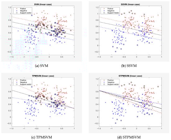
Figure 1. Results on Example 1 (Ripley’s dataset, linear case).

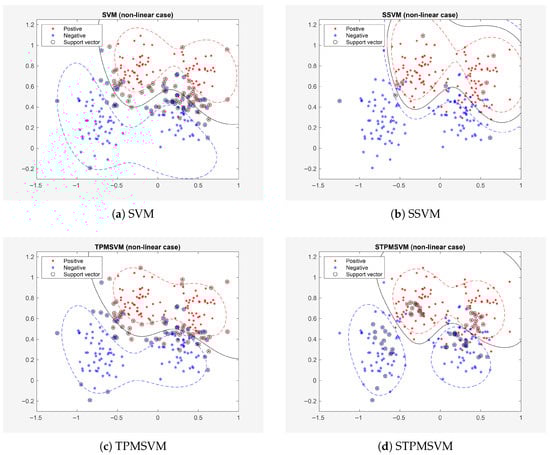
Figure 2. Results on Example 1 (Ripley’s dataset, non-linear case).

Table 3. Final Final results on Example 1 (Ripley’s dataset).

Kernel Type	Item	SVM	SSVM	TPMSVM	STPMSVM
Linear kernel	Acc.(%)	89.70	89.70	88.80	88.80
	Num-SVs	110	14 (↓87.27%)	83	17 (↓79.52%)
	Tr-time(s)	0.2040	0.1929	0.3296	0.3171
	Te-time(s)	0.0325	0.0072	0.0744	0.0142
Gaussian kernel	Acc.(%)	90.40	90.60	91.20	91.40
	Num-SVs	96	10 (↓89.58%)	82	57 (↓30.49%)
	Tr-time(s)	0.2316	0.2087	0.4073	0.3140
	Te-time(s)	0.0261	0.0090	0.0677	0.0509

Note: 1. Acc. (prediction accuracy); Num-SVs (number of support vectors); Tr-time (training time); Te-time (testing time). These abbreviations are used consistently in subsequent tables. 2. ↓ represents the percentage decrease in the number of support vectors compared to the baseline. 3. A minimal reproducibility package for the non-linear case is provided in the Supplementary Materials.

As shown in Figure 1 and Figure 2 and Table 3, both SSVM and STPMSVM exhibit a reduction in the number of suport vectors, training time and testing time—without compromising prediction accuracy—in comparison to the traditional methods under both linear and nonlinear settings. Specifically, in the linear case, SSVM reduces the number of support vectors by 87.27% compared with SVM, and STPMSVM reduces 79.52% compared with TPMSVM; in the nonlinear case, the reductions are 89.58% and 30.49%, respectively. These quantitative results clearly demonstrate the sparsity of the proposed methods. It should also be noted that SSVM outperforms SVM in terms of accuracy. In fact, STPMSVM not only matches the performance of other algorithms but also attains the highest accuracy in both linear and nonlinear scenarios. Furthermore, all four algorithms demonstrate improved accuracy in nonlinear cases compared to linear cases. In addition, SSVM requires the fewest SVs and the shortest training and testing times in this experiment, and STPMSVM delivers the best comprehensive performance.

Moreover, we observe that the SVs of SSVM and STPMSVM (see Figure 1 and Figure 2) are not within the margins as they are in the corresponding traditional methods. Instead, they represent some “prototype” points from the datasets. This occurs because $\alpha$ (in SSVM), ${\alpha }_{+}$ and ${\alpha }_{-}$ (in STPMSVM) are no longer the original dual variables in our new sparse model. This is a distinct difference between our sparse methods and classical methods.

The sparsity of the proposed models can also be interpreted from a geometric perspective. In the conventional SVM and TPMSVM, support vectors include not only those on the margin boundary but also those inside the margin and misclassified samples beyond it. As a result, the margin-maximization principle inherently leads to a relatively large number of support vectors, limiting the sparsity of the model. In contrast, the proposed sparse models select class prototype vectors as support vectors, whose quantity is not constrained by the large-margin principle. This allows the models to achieve high sparsity with only a small set of representative support vectors.

4.2.2. Example 2

The second example we consider is still a two-dimensional synthetic dataset (denoted as A0), where data of the two classes is randomly generated as follows.

• Class +1: $x_{+}\sim U\left[-{\displaystyle \frac{\pi }{2}},{\displaystyle \frac{3\pi }{2}}\right],y_{+}=0.8sin\left(x_{+}\right)-0.25+0.6\epsilon$, where $\epsilon \sim U(0,1)$,
• Class −1: $\theta \in [0,\pi ],r=\sqrt{2u},u\sim U(0,1)$, $x_{-}=rcos\theta +1.5,y_{-}=rsin\theta -1-c$, where $c\sim N(0,0.01)$ is Gaussian noise.

The tuning set consists of 200 points (balanced across the two classes), and the training/testing set contains 200 points (also balanced). The results are illustrated in Figure 3 and summarized in Table 4 (The results reported in the following table are presented as “mean ± variance” over the 10 folds. It is evident that, while maintaining prediction accuracy, SSVM and STPMSVM have significantly fewer support vectors and require shorter training time and testing time compared to SVM and TPMSVM, respectively.

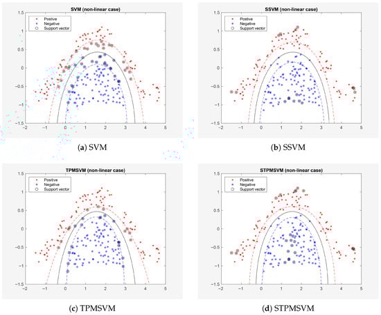
Figure 3. Results on Example 2 (Dataset A0).

Table 4. Results on Example 2.

Dataset	SVM	SSVM	TPMSVM	STPMSVM
	Acc.(%)	Acc.(%)	Acc.(%)	Acc.(%)
	Num-SVs	Num-SVs	Num-SVs	Num-SVs
	Tr-Time(s)	Tr-Time(s)	Tr-Time(s)	Tr-Time(s)
	Te-Time(s)	Te-Time(s)	Te-Time(s)	Te-Time(s)
A0	98.50 ± 2.42	98.50 ± 3.37	99.50 ± 1.58	99.50 ± 0.79
	43.20 ± 0.23	16.10 ± 0.74	25.20 ± 1.81	21.90 ± 1.37
	0.2312 ± 0.0238	0.1949 ± 0.0073	0.3808 ±0.0160	0.3158 ± 0.0207
	0.0006 ± 0.0002	0.0005 ± 0.0002	0.0009 ±0.0004	0.0008 ± 0.0003
A1	99.00 ± 2.11	99.00 ± 2.11	99.50 ± 1.58	99.00 ± 2.11
	86.10 ± 1.52	27.20 ± 0.92	22.10 ± 1.79	21.60 ± 1.17
	0.2189 ± 0.0150	0.1893 ± 0.0135	0.3169 ± 0.0116	0.3169 ± 0.0116
	0.0009 ± 0.0002	0.0003 ± 0.0001	0.0010 ±0.0003	0.0008 ± 0.0003
A2	99.00 ± 3.16	99.00 ± 3.16	98.50 ± 3.37	99.00 ± 3.16
	118.10 ± 1.85	37.90 ± 1.29	23.20 ± 2.49	22.20 ± 0.92
	0.2257 ± 0.0113	0.1899 ± 0.0062	0.3973 ± 0.0925	0.3448 ± 0.0325
	0.0012 ± 0.0002	0.0004 ± 0.0003	0.0010 ±0.0002	0.0009 ± 0.0002
A3	99.00 ± 2.11	99.50 ± 1.58	99.00 ± 2.11	99.00 ± 2.11
	34.60 ± 1.58	26.70 ± 0.95	24.20 ± 1.81	22.80 ± 1.93
	0.2259 ± 0.0194	0.1895 ± 0.0077	0.4156 ± 0.0319	0.3142 ± 0.0092
	0.0005 ± 0.0002	0.0005 ± 0.0002	0.0010 ±0.0003	0.0007 ± 0.0002
A4	98.00 ± 2.58	98.50 ± 2.42	98.50 ± 2.42	98.50 ± 2.42
	64.60 ± 1.26	24.40 ± 0.70	24.60 ± 2.01	22.30 ± 1.70
	0.2277 ± 0.0150	0.1917 ± 0.0116	0.4100 ± 0.0647	0.3230 ± 0.0105
	0.0006 ± 0.0001	0.0004 ± 0.0002	0.0011 ±0.0002	0.0008 ± 0.0002
A5	96.50 ± 4.12	96.50 ± 4.12	96.00 ± 5.16	96.00 ± 5.16
	122.80 ± 2.04	23.90 ± 0.88	22.70 ± 0.95	20.80 ± 0.63
	0.2169 ± 0.0133	0.1965 ± 0.0125	0.3781 ± 0.0200	0.3373 ± 0.0453
	0.0011 ± 0.0001	0.0005 ± 0.0002	0.0010 ±0.0005	0.0007 ± 0.0003
A6	95.50 ± 3.69	95.00 ± 6.24	93.50 ± 5.80	93.50 ± 5.80
	27.60 ± 2.55	24.50 ± 1.43	25.80 ± 1.32	21.60 ± 0.70
	0.2667 ± 0.0209	0.1926 ± 0.0056	0.3871 ± 0.0436	0.3111 ± 0.0134
	0.0004 ± 0.0002	0.0004 ± 0.0004	0.0011 ±0.0003	0.0009 ± 0.0002
A7	88.50 ± 9.14	86.50 ± 10.01	88.50 ± 9.14	89.50 ± 7.98
	45.30 ± 3.47	33.50 ± 1.27	25.50 ± 2.32	22.70 ± 1.25
	0.2401 ± 0.0297	0.1936 ± 0.0095	0.3878 ± 0.0084	0.3860 ± 0.0059
	0.0005 ± 0.0002	0.0005 ± 0.0002	0.0010 ±0.0005	0.0010 ± 0.0004
A8	80.50 ± 9.26	80.50 ± 8.32	79.50 ± 6.43	80.50 ± 9.56
	130.70 ± 2.26	21.50 ± 0.53	29.00 ± 2.45	26.70 ± 3.56
	0.2200 ± 0.0148	0.2018 ± 0.0175	0.3972 ± 0.0212	0.3100 ± 0.0130
	0.0010 ± 0.0002	0.0006 ± 0.0002	0.0010 ±0.0001	0.0009 ± 0.0001
A9	74.00 ± 7.38	73.50 ± 8.51	74.50 ± 8.32	75.50 ± 8.32
	96.10 ± 3.51	10.50 ± 0.97	70.10 ± 12.00	30.10 ± 5.74
	0.2245 ± 0.0192	0.1974 ± 0.0145	0.4160 ± 0.0765	0.3088 ± 0.0099
	0.0008 ± 0.0002	0.0003 ± 0.0001	0.0013 ±0.0008	0.0010 ± 0.0002
Avg. SV-Reduction (%)	—	57.46	—	13.54
p-value/r (Acc.)	a 0.7500/0.1008	c 0.5313/0.4168	b 0.1875/0.4168
p-value/r (Num-SVs)	a,* 0.0488/0.6230 (SSVM < SVM)	c 0.2324/0.3776	b,* 0.0020/0.9794 (STPMSVM < TPMSVM)
p-value/r (Tr-time)	a,* 0.0488/0.6230 (SSVM < SVM)	c 0.2324/0.3776	b,* 0.0020/0.9794 (STPMSVM < TPMSVM)
p-value/r (Te-time)	a,* 0.0156/0.7645 (SSVM < SVM)	c,* 0.0020/0.9794 (SSVM < STPMSVM)	b,* 0.0039/0.9125 (STPMSVM < TPMSVM)

Note: 1. The letters “a”, “b”, and “c” denote the W-test results for the SVM vs. SSVM, TPMSVM vs. STPMSVM, and SSVM vs. STPMSVM pairings, respectively. 2. The asterisk (*) indicates statistical significance at the level of $p<0.05$. 3. For significant results, the directional notation indicates which model had a larger median value. Performance interpretation depends on the metric. 4. The same notations apply to subsequent tables.

To examine the noise resistance of our proposed sparse methods, we conducted experiments on 9 datasets with different noise intensity based on dataset A0, denoted as A1–A9. For each point of dataset A0, we add different noise vectors, all following normal distributions with mean $\mu =[0;0]$ and covariance matrices ${\Sigma }_1=\left[\begin{array}{cc}0.001& 0\\ 0& 0.001\end{array}\right]$, ${\Sigma }_2=\left[\begin{array}{cc}0.0025& 0\\ 0& 0.0025\end{array}\right]$, ${\Sigma }_3=\left[\begin{array}{cc}0.005& 0\\ 0& 0.005\end{array}\right]$, ${\Sigma }_4=\left[\begin{array}{cc}0.01& 0\\ 0& 0.01\end{array}\right]$, ${\Sigma }_5=\left[\begin{array}{cc}0.025& 0\\ 0& 0.025\end{array}\right]$, ${\Sigma }_6=\left[\begin{array}{cc}0.05& 0\\ 0& 0.05\end{array}\right]$, ${\Sigma }_7=\left[\begin{array}{cc}0.1& 0\\ 0& 0.1\end{array}\right]$, ${\Sigma }_8=\left[\begin{array}{cc}0.25& 0\\ 0& 0.25\end{array}\right]$, and ${\Sigma }_9=\left[\begin{array}{cc}0.5& 0\\ 0& 0.5\end{array}\right]$, respectively. The results are also reported in Table 3. The bottom of Table 3 provides the corresponding Wilcoxon test results, including p-values and effect sizes (denoted as r; the same presentation is used in the subsequent tables). In addition, the average percentage reductions in the number of support vectors (Avg. SV-Reduction) of the sparse models compared with their baseline counterparts are presented to quantitatively demonstrate the sparsity improvement.

As we can see from Table 4 and Figure 3, the sparse models significantly reduce the number of support vectors (with SSVM and STPMSVM achieving average reductions of 57.46% and 13.54%, respectively, compared with the baseline models), as well as training and prediction times, while maintaining comparable prediction accuracy. Moreover, as noise intensity increases, STPMSVM demonstrates a more pronounced advantage in prediction accuracy, whereas SSVM achieves the shortest training and testing times. A detailed comparison shows that SSVM’s accuracy degrades relative to STPMSVM at higher noise levels, even when Wilcoxon tests are not statistically significant. This degradation is mainly caused by SSVM’s very small number of support vectors, which can induce underfitting and reduce its ability to capture noisy structure. By contrast, STPMSVM retains a more flexible decision boundary and a larger set of prototype points (support vectors), yielding stronger generalization and greater stability under noise—consistent with our theoretical expectations. Overall, STPMSVM is more robust to noise contamination.

To further test the performance stability of our method, we generate another 15 datasets consisting of 200 points with the same distribution as datasets A0 and A7, respectively, and the same number of samples for both classes. The results are shown in Table 5 and Table 6, respectively. At the bottom of the two tables, in addition to the previously reported Wilcoxon test results and average support vector reduction percentages, means, standard deviations (Std) and the medians (Med) of the four performance metrics for the four models are also reported, providing a more comprehensive comparison.

Table 5. Results on 16 datasets with the same distribution of dataset A0.

Dataset	SVM	SSVM	TPMSVM	STPMSVM
	Acc.(%)	Acc.(%)	Acc.(%)	Acc.(%)
	Num-SVs	Num-SVs	Num-SVs	Num-SVs
	Tr-Time(s)	Tr-Time(s)	Tr-Time(s)	Tr-Time(s)
	Te-Time(s)	Te-Time(s)	Te-Time(s)	Te-Time(s)
A0	98.50 ± 2.42	98.50 ± 3.37	99.50 ± 1.58	99.50 ± 0.79
	43.20 ± 0.23	16.10 ± 0.74	25.20 ± 1.81	21.90 ± 1.37
	0.2312 ± 0.0238	0.1949 ± 0.0073	0.3808 ±0.0160	0.3158 ± 0.0207
	0.0006 ± 0.0002	0.0005 ± 0.0002	0.0009 ±0.0004	0.0008 ± 0.0003
1st	99.50 ± 1.58	98.00 ± 2.58	99.50 ± 1.58	100.00 ± 0
	48.20 ± 1.03	37.50 ± 0.85	40.20 ± 1.87	25.60 ± 0.70
	0.2183 ± 0.0092	0.1933 ± 0.0107	0.3785 ± 0.0260	0.2964 ± 0.0107
	0.0006 ± 0.0003	0.0003 ± 0.0002	0.0013 ± 0.0007	0.0010 ± 0.0002
2nd	99.00 ± 2.11	99.50 ± 1.58	100.00 ± 0	99.50 ± 1.58
	95.70 ± 1.83	30.00 ± 1.15	25.20 ± 2.66	22.30 ± 1.57
	0.2364 ± 0.0120	0.1869 ± 0.0091	0.4617 ± 0.0295	0.3005 ± 0.0131
	0.0010 ± 0.0002	0.0004 ± 0.0002	0.0012 ±0.0004	0.0008 ± 0.0003
3rd	100.00 ± 0	100.00 ± 0	99.00 ± 1.58	100.00 ± 0
	86.70 ± 1.89	25.40 ± 0.97	41.60 ± 0.97	22.50 ± 1.51
	0.2313 ± 0.0151	0.1930 ± 0.0134	0.3657 ± 0.0078	0.2915 ± 0.0120
	0.0009 ± 0.0002	0.0004 ± 0.0001	0.0011 ±0.0002	0.0009 ± 0.0001
4th	99.00 ± 3.16	100.00 ± 0	100.00 ± 0	100.00 ± 0
	87.80 ± 2.35	17.80 ± 0.92	26.30 ± 1.95	21.20 ± 0.92
	0.2526 ± 0.0268	0.2353 ± 0.0169	0.3748 ± 0.0239	0.3015 ± 0.0097
	0.0011 ± 0.0003	0.0004 ± 0.0001	0.0011 ± 0.0002	0.0009 ± 0.0002
5th	98.00 ± 3.50	99.00 ± 3.37	99.50 ± 1.58	99.50 ± 1.58
	87.60 ± 1.96	17.40 ± 0.52	23.20 ± 1.55	22.10 ± 1.37
	0.2449 ± 0.0187	0.2417 ± 0.0177	0.3672 ±0.0153	0.2975 ± 0.0128
	0.0010 ± 0.0001	0.0005 ± 0.0002	0.0010 ±0.0002	0.0009 ± 0.0001
6th	99.00 ± 2.11	99.50 ± 1.58	99.50 ± 1.58	99.50 ± 1.58
	23.70 ± 0.67	18.60 ± 1.07	23.00 ± 2.11	22.40 ± 1.26
	0.2367 ± 0.0145	0.2002 ± 0.0090	0.3619 ± 0.0094	0.2872 ± 0.0101
	0.0004 ± 0.0003	0.0003 ± 0.0002	0.0010 ± 0.0002	0.0010 ± 0.0002
7th	100.00 ± 0	100.00 ± 0	100.00 ± 0	100.00 ± 0
	32.50 ± 0.85	21.20 ± 0.79	25.30 ± 3.40	22.90 ± 1.10
	0.2615 ± 0.0506	0.1903 ± 0.0088	0.3841 ± 0.0569	0.2938 ± 0.0115
	0.0005 ± 0.0002	0.0003 ± 0.0001	0.0010 ±0.0002	0.0008 ± 0.0003
8th	98.00 ± 3.50	99.00 ± 3.16	98.50 ± 3.37	98.50 ± 3.37
	86.50 ± 1.84	25.70 ± 1.06	23.40 ± 1.07	25.60 ± 0.97
	0.2435 ± 0.0221	0.2068 ± 0.0070	0.3658 ± 0.0069	0.3058 ± 0.0184
	0.0010 ± 0.0002	0.0004 ± 0.0002	0.0010 ±0.0004	0.0008 ± 0.0002
9th	99.50 ± 1.58	99.50 ± 1.58	99.50 ± 1.58	99.50 ± 1.58
	83.30 ± 1.06	25.90 ± 0.74	21.80 ± 1.62	21.40 ± 1.26
	0.2432 ± 0.0124	0.2219 ± 0.0340	0.3911 ± 0.0563	0.2975 ± 0.0091
	0.0010 ± 0.0002	0.0004 ± 0.0002	0.0011 ±0.0003	0.0008 ± 0.0003
10th	97.00 ± 4.83	97.00 ± 4.83	98.50 ± 2.42	98.00 ± 3.50
	72.30 ± 1.89	39.00 ± 0.94	24.90 ± 1.79	22.20 ± 1.93
	0.2139 ± 0.0092	0.2138 ± 0.0120	0.3918 ± 0.0479	0.3098 ± 0.0169
	0.0006 ± 0.0001	0.0004 ± 0.0002	0.0011 ±0.0002	0.0006 ± 0.0002
11th	98.00 ± 2.58	99.00 ± 2.11	99.50 ± 1.58	99.50 ± 1.58
	113.60 ± 1.26	28.00 ± 0.82	27.60 ± 1.58	21.50 ± 1.18
	0.2110 ± 0.0119	0.2110 ± 0.0146	0.3911 ± 0.0228	0.2990 ± 0.0195
	0.0008 ± 0.0003	0.0003 ± 0.0002	0.0012 ±0.0003	0.0012 ± 0.0003
12th	97.00 ± 4.22	98.50 ± 2.42	99.00 ± 2.11	98.00 ± 2.58
	85.20 ± 1.32	25.60 ± 0.97	23.10 ± 1.37	22.60 ± 1.96
	0.2194 ± 0.0170	0.1961 ± 0.0144	0.4142 ± 0.0349	0.3030 ± 0.0200
	0.0007 ± 0.0003	0.0004 ± 0.0002	0.0011 ±0.0003	0.0010 ± 0.0002
13th	97.50 ± 2.64	99.50 ± 1.58	99.00 ± 2.11	98.50 ± 2.42
	94.10 ± 1.66	7.70 ± 0.67	24.90 ± 1.73	21.10 ± 0.88
	0.2286 ± 0.0183	0.2040 ± 0.0125	0.4126 ± 0.0307	0.3095 ± 0.0226
	0.0008 ± 0.0002	0.0004 ± 0.0002	0.0011 ±0.0004	0.0009 ± 0.0002
14th	96.00 ± 3.94	98.00 ± 2.58	99.50 ± 1.58	99.00 ± 2.11
	117.60 ± 1.58	39.90 ± 0.74	57.50 ± 1.43	23.10 ± 1.79
	0.2349 ± 0.0189	0.2070 ± 0.0124	0.4410 ± 0.0532	0.2958 ± 0.0138
	0.0008 ± 0.0002	0.0005 ± 0.0002	0.0014 ±0.0009	0.0011 ± 0.0002
15th	99.50 ± 1.58	100.00 ± 0	99.00 ± 3.16	99.50 ± 1.58
	90.10 ± 1.52	39.90 ± 0.88	23.60 ± 2.37	23.20 ± 1.48
	0.2233 ± 0.0141	0.1990 ± 0.0048	0.4393 ± 0.0446	0.3031 ± 0.0110
	0.0008 ± 0.0003	0.0004 ± 0.0002	0.0010 ±0.0002	0.0010 ± 0.0002
Mean/Std/Med(Acc.)	98.47/1.18/98.75	99.06/0.87/99.25	99.34/0.47/99.50	99.28/0.68/99.50
Mean/Std/Med(Num-SVs)	78.32/27.32/87.15	25.98/9.52/25.65	28.55/9.65/25.05	22.60/1.33/22.35
Mean/Std/Med(Tr-ime)	0.2332/0.0140/0.2333	0.2054/0.0162/0.2021	0.3952/0.0303/0.3876	0.3000/0.0080/0.2990
Mean/Std/Med(Te-ime)	0.0008/0.0002/0.0008	0.0004/0.0000/0.0004	0.0011/0.0001/0.0011	0.0009/0.0001/0.0009
Avg. SV-Reduction (%)	—	61.65	—	15.46
p-value/r (Acc.)	a,* 0.0254/0.5589 (SSVM > SVM)	c 0.3086/0.2545	b 0.7891/0.0669
p-value/r (Num-SVs)	a,* 0.0004/0.8790 (SSVM < SVM)	c 0.1960/0.3232	b,* 0.0013/0.8016 (STPMSVM < TPMSVM)
p-value/r (Tr-time)	a,* 0.0001/0.9998 (SSVM < SVM)	c,* 0.0004/0.8790 (SSVM < STPMSVM)	b,* 0.0004/0.8790 (STPMSVM < TPMSVM)
p-value/r (Te-time)	a,* 0.0004/0.8813 (SSVM < SVM)	c,* 0.0004/0.8827 (SSVM < STPMSVM)	b,* 0.0004/0.9171 (STPMSVM < TPMSVM)

Table 6. Results on 16 datasets with the same distribution of dataset A7.

Dataset	SVM	SSVM	TPMSVM	STPMSVM
	Acc.(%)	Acc.(%)	Acc.(%)	Acc.(%)
	Num-SVs	Num-SVs	Num-SVs	Num-SVs
	Tr-Time(s)	Tr-Time(s)	Tr-Time(s)	Tr-Time(s)
	Te-Time(s)	Te-Time(s)	Te-Time(s)	Te-Time(s)
A7	88.50 ± 9.14	86.50 ± 10.01	88.50 ± 9.14	89.50 ± 7.98
	45.30 ± 3.47	33.50 ± 1.27	25.50 ± 2.32	22.70 ± 1.25
	0.2401 ± 0.0297	0.1936 ± 0.0095	0.3878 ± 0.0084	0.3860 ± 0.0059
	0.0005 ± 0.0002	0.0005 ± 0.0002	0.0010 ±0.0005	0.0010 ± 0.0004
1st	92.00 ± 4.83	91.00 ± 4.59	91.50 ± 4.47	92.50 ± 5.40
	92.00 ± 1.94	34.40 ± 1.26	58.00 ± 1.89	39.60 ± 1.07
	0.2543 ± 0.0177	0.1834 ± 0.0077	0.3597 ± 0.0149	0.2934 ± 0.0068
	0.0010 ± 0.0003	0.0003 ± 0.0002	0.0012 ±0.0002	0.0010 ± 0.0002
2nd	93.50 ± 6.26	92.50 ± 5.89	93.50 ± 5.80	94.00 ± 6.15
	49.60 ± 1.78	29.90 ± 0.74	23.50 ± 1.58	22.80 ± 0.92
	0.2548 ± 0.0169	0.1870 ± 0.0097	0.3804 ± 0.0288	0.3768 ± 0.0132
	0.0007 ± 0.0003	0.0002 ± 0.0002	0.0010 ±0.0002	0.0008 ± 0.0002
3rd	89.00 ± 7.75	90.00 ± 6.67	89.50 ± 6.43	90.00 ± 6.67
	49.10 ± 2.02	18.80 ± 0.63	24.60 ± 2.17	21.50 ± 1.58
	0.2092 ± 0.0204	0.1716 ± 0.0094	0.4350 ± 0.0643	0.3967 ± 0.0095
	0.0005 ± 0.0002	0.0002 ± 0.0001	0.0011 ±0.0003	0.0010 ± 0.0003
4th	90.00 ± 6.24	90.00 ± 6.24	89.00 ± 6.99	89.00 ± 5.16
	101.20 ± 2.15	6.30 ± 0.67	62.60 ± 1.43	23.70 ± 2.50
	0.2095 ± 0.0089	0.2002 ± 0.0269	0.3652 ± 0.0102	0.2950 ± 0.0074
	0.0008 ± 0.0002	0.0004 ± 0.0003	0.0012 ±0.0003	0.0007 ± 0.0003
5th	88.50 ± 5.80	88.00 ± 7.53	87.00 ± 5.87	87.50 ± 7.17
	50.90 ± 2.85	33.30 ± 0.82	50.20 ± 2.39	24.90 ± 3.00
	0.2387 ± 0.0179	0.1787 ± 0.0065	0.3777 ± 0.0313	0.3053 ± 0.0219
	0.0005 ± 0.0002	0.0005 ± 0.0002	0.0011 ±0.0001	0.0010 ± 0.0002
6th	90.00 ± 6.24	90.00 ± 5.77	89.00 ± 5.68	90.50 ± 6.85
	128.50 ± 1.72	8.70 ± 0.95	23.30 ± 1.89	25.30 ± 1.70
	0.2219 ± 0.0278	0.1708 ± 0.0066	0.3692 ± 0.0105	0.3088 ± 0.0121
	0.0011 ± 0.0003	0.0006 ± 0.0002	0.0011 ±0.0002	0.0009 ± 0.0003
7th	92.50 ± 5.40	91.50 ± 5.80	91.00 ± 5.16	92.00 ± 5.87
	83.90 ± 2.13	19.10 ± 0.57	22.80 ± 2.20	22.70 ± 1.77
	0.2237 ± 0.0132	0.1772 ± 0.0130	0.3944 ± 0.0322	0.3794 ± 0.0163
	0.0007 ± 0.0001	0.0005 ± 0.0001	0.0010 ±0.0002	0.0008 ± 0.0005
8th	89.50 ± 5.99	88.00 ± 7.15	91.50 ± 5.30	91.00 ± 6.15
	103.30 ± 1.83	30.30 ± 0.95	23.20 ± 1.81	23.80 ± 2.15
	0.2140 ± 0.0152	0.1748 ± 0.0126	0.3890 ± 0.0305	0.3701 ± 0.0404
	0.0008 ± 0.0002	0.0003 ± 0.0002	0.0010 ±0.0003	0.0008 ± 0.0004
9th	93.00 ± 4.22	93.50 ± 4.47	92.50 ± 4.25	92.00 ± 4.22
	45.30 ± 2.45	27.20 ± 1.03	25.00 ± 2.31	21.70 ± 1.16
	0.2138 ± 0.0113	0.1785 ± 0.0085	0.3855 ± 0.0218	0.2964 ± 0.0115
	0.0005 ± 0.0002	0.0004 ± 0.0002	0.0010 ±0.0003	0.0010 ± 0.0001
10th	89.50 ± 9.85	88.50 ± 8.18	88.50 ± 10.55	90.00 ± 9.43
	124.30 ± 2.83	15.80 ± 1.14	39.50 ± 0.85	26.40 ± 4.58
	0.2131 ± 0.0152	0.1769 ± 0.0087	0.4439 ± 0.0477	0.2923 ± 0.0072
	0.0010 ± 0.0002	0.0003 ± 0.0001	0.0012 ±0.0004	0.0008 ± 0.0001
11th	91.50 ± 4.12	90.50 ± 4.38	92.50 ± 4.86	91.00 ± 5.16
	115.90 ± 1.29	5.40 ± 0.70	25.90 ± 1.52	22.70 ± 1.83
	0.2479 ± 0.0158	0.1943 ± 0.0334	0.3782 ± 0.0163	0.2994 ± 0.0228
	0.0011 ± 0.0002	0.0003 ± 0.0002	0.0011 ±0.0002	0.0011 ± 0.0003
12th	90.00 ± 7.45	89.50 ± 7.25	88.50 ± 9.44	91.00 ± 6.58
	57.00 ± 2.83	12.00 ± 0.67	29.10 ± 1.45	22.60 ± 1.84
	0.2439 ± 0.0189	0.2354 ± 0.0161	0.3731 ± 0.0193	0.2996 ± 0.0115
	0.0007 ± 0.0002	0.0003 ± 0.0002	0.0010 ±0.0002	0.0009 ± 0.0002
13th	88.50 ± 5.30	87.00 ± 5.37	88.50 ± 4.74	88.50 ± 4.74
	81.40 ± 2.07	9.20 ± 0.92	21.90 ± 1.37	22.20 ± 1.32
	0.2224 ± 0.0132	0.1848 ± 0.0085	0.3605 ± 0.0130	0.2977 ± 0.0156
	0.0007 ± 0.0001	0.0003 ± 0.0002	0.0011 ±0.0002	0.0009 ± 0.0003
14th	88.00 ± 6.32	90.50 ± 4.38	90.50 ± 4.38	88.50 ± 6.69
	48.00 ± 2.75	28.70 ± 0.82	24.50 ± 1.18	22.50 ± 1.08
	0.2761 ± 0.0282	0.1878 ± 0.0081	0.3787 ± 0.0312	0.3668 ± 0.0620
	0.0006 ± 0.0003	0.0002 ± 0.0001	0.0011 ±0.0002	0.0010 ± 0.0003
15th	89.50 ± 5.50	89.50 ± 8.64	89.00 ± 8.43	90.00 ± 5.27
	117.90 ± 2.33	19.20 ± 1.23	40.00 ± 2.40	26.40 ± 1.71
	0.2206 ± 0.0147	0.1965 ± 0.0068	0.3885 ± 0.0392	0.2967 ± 0.0083
	0.0009 ± 0.0002	0.0004 ± 0.0002	0.0012 ±0.0002	0.0010 ± 0.0002
Mean/Std/Med(Acc.)	90.22/1.74/89.75	89.78/1.89/90	89.91/2.03/89.25	90.53/1.64/90.50
Mean/Std/Med(Num-SVs)	80.85/31.48/82.56	20.74/10.39/19.15	33.13/13.17/25.70	24.47/4.32/22.75
Mean/Std/Med(Tr-ime)	0.2177/0.0612/0.2228	0.1870/0.0157/0.1841	0.3855/0.0235/0.3796	0.3240/0.03838/0.3025
Mean/Std/Med(Te-ime)	0.0008/0.0002/0.0007	0.0004/0.0001/0.0003	0.0010/0.0000/0.0011	0.0009/0.0001/0.0010
Avg. SV-Reduction (%)	—	67.11	—	19.67
p-value/r (Acc.)	a 0.0728/0.4228	c,* 0.0334/0.5015 (STPMSVM > SVM)	b,* 0.0419/0.4797 (STPMSVM > TPMSVM)
p-value/r (Num-SVs)	a,* 0.0004/0.8790 (SSVM < SVM)	c 0.1960/0.3232	b,* 0.0015/0.7952 (STPMSVM < TPMSVM)
p-value/r (Tr-time)	a,* 0.0033/0.6929 (SSVM < SVM)	c,* 0.0002/0.8770 (SSVM < STPMSVM)	b,* 0.0003/0.8469 (STPMSVM < TPMSVM)
p-value/r (Te-time)	a,* 0.0004/0.9331 (SSVM < SVM)	c,* 0.0001/0.9056 (SSVM < STPMSVM)	b,* 0.0002/0.8713 (STPMSVM < TPMSVM)

From Table 5 and Table 6, it is evident that, overall, under both conditions, the sparse methods significantly outperform their corresponding traditional counterparts in all other metrics while maintaining comparable prediction accuracy, and SSVM exhibits the highest prediction efficiency. In particular, in the two scenarios, the average number of support vectors was reduced by 15.46% and 19.67% for STPMSVM, and by 61.65% and 67.11% for SSVM, respectively, compared with their baseline models. The mean values of accuracy reveal a trend: on the 15 datasets sharing the same distribution as A0, SSVM achieves noticeably higher accuracy than SVM, while STPMSVM attains nearly identical accuracy to TPMSVM. On the 15 noisy datasets derived from A7, however, STPMSVM achieves the highest mean prediction accuracy among the four algorithms. This is consistent with the previous results, demonstrating that STPMSVM maintains greater robustness under strong noise conditions. Overall, STPMSVM demonstrates strong sparsity, and stable predictive performance under both noiseless and high-noise conditions, while SSVM achieves the highest prediction efficiency and better accuracy than SVM under low noise conditions. Thus, STPMSVM is more robust and delivers the best overall performance.

To investigate the performance trends of the proposed models as the number of training samples increases, we generate training and test sets independently following the same distributions as datasets A2 (low noise) and A8 (strong noise). The training set sizes are gradually increased from 200 to 2000 in steps of 200, while the testing set is fixed at 600 samples for each case. For each training set, the models are trained once and evaluated on the corresponding fixed test set. The results are presented in Figure 4 and Figure 5.

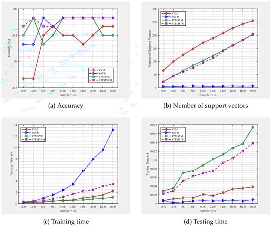
Figure 4. Performance of four algorithms under different training sample sizes, following the same distribution as A2.

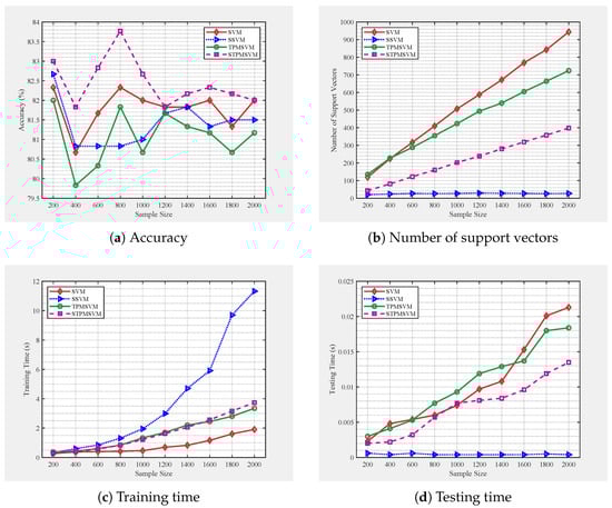
Figure 5. Performance of four algorithms under different training sample sizes, following the same distribution as A8.

From Figure 4 and Figure 5, we observe clear performance trends as the number of training samples increases. Both SSVM and STPMSVM produce consistently fewer support vectors than their respective baselines (SVM and TPMSVM), with SSVM achieving the highest sparsity and exhibiting a stable number of support vectors that remain nearly unchanged with growing sample size. This confirms that the proposed models effectively enhance sparsity through their structural reformulation. The reduced number of support vectors directly leads to faster prediction speed. Moreover, SSVM achieves the lowest and most consistent testing time, while the other methods show increasing prediction cost as the training size grows. This efficiency improvement stems from the sparsity induced by the LPPs. In contrast, TPMSVM exhibits the fastest increase in prediction time under low-noise conditions, whereas under high noise, SVM becomes slower in prediction speed due to reduced margin robustness. Regarding training time, SSVM increases most rapidly with sample size, reflecting its higher computational complexity, whereas STPMSVM achieves a moderate trade-off—slightly higher than TPMSVM under low noise but comparable under high noise. Although STPMSVM incurs a somewhat higher cost, its linear formulation and sparsity contribute to balanced learning efficiency. In terms of generalization performance, under low noise conditions both sparse models perform comparably or better than their baselines. Under high noise, STPMSVM maintains the best accuracy, while SSVM shows performance degradation due to excessive sparsity, indicating mild underfitting. Overall, SSVM offers superior sparsity and prediction efficiency, whereas STPMSVM achieves the most favorable balance among sparsity, robustness, and generalization stability as sample scale increases.

4.2.3. Extension of Example 2: Increased Complexity Experiments

To further comprehensively evaluate the robustness of the proposed sparse models under different types of noise perturbations, we design three groups of experiments: label noise, class imbalance, and heteroscedastic noise. All sets are independently generated from the same distribution.

Label noise: Based on the distributions of A0 and A5, we randomly flip the labels of both classes with rates of 0%, 5%, 10%, and 15%. The resulting training sets are denoted as A0-00, A0-05, A0-10, A0-15, A5-00, A5-05, A5-10, and A5-15. For each set, the tuning set and the training set contain 400 samples, respectively, with both classes equally balanced. The results are shown in Table 7 (in order to provide a more comprehensive evaluation of model performance, we also report the Brier score in Table 7, Table 8 and Table 9).

Table 7. Results on label flipping datasets.

Dataset	SVM	SSVM	TPMSVM	STPMSVM
	Acc.(%)	Acc.(%)	Acc.(%)	Acc.(%)
	Num-SVs	Num-SVs	Num-SVs	Num-SVs
	Tr-Time(s)	Tr-Time(s)	Tr-Time(s)	Tr-Time(s)
	Te-Time(s)	Te-Time(s)	Te-Time(s)	Te-Time(s)
A0-00	99.75 ± 0.79	99.25 ± 1.69	99.75 ± 0.79	100.00 ± 0.00
	30.00 ± 1.56	39.90 ± 0.99	42.90 ± 0.88	38.60 ± 0.70
	0.2497 ± 0.0320	0.3924 ± 0.0271	0.3932 ± 0.0279	0.3588 ± 0.0207
	0.0009 ± 0.0014	0.0004 ± 0.0002	0.0006 ± 0.0004	0.0004 ± 0.0003
	0.3134	0.3169	0.3262	0.3151
A0-05	94.00 ± 3.37	95.00 ± 2.64	95.00 ± 2.64	95.00 ± 2.64
	104.70 ± 4.67	7.00 ± 0.47	40.50 ± 1.08	39.20 ± 0.92
	0.2571 ± 0.0289	0.4188 ± 0.0205	0.3470 ± 0.0283	0.3475 ± 0.0133
	0.0007 ± 0.0004	0.0003 ± 0.0002	0.0007 ± 0.0002	0.0005 ± 0.0001
	0.3124	0.3151	0.3158	0.3122
A0-10	87.75 ± 5.33	88.00 ± 5.11	85.00 ± 5.00	86.25 ± 5.66
	193.00 ± 1.78	22.00 ± 0.82	77.20 ± 2.15	74.60 ± 0.70
	0.2073 ± 0.0125	0.3631 ± 0.0157	0.3354 ± 0.0152	0.3407 ± 0.0082
	0.0006 ± 0.0003	0.0004 ± 0.0002	0.0006 ± 0.0003	0.0004 ± 0.0000
	0.3119	0.3123	0.3167	0.3131
A0-15	84.25 ± 6.46	84.50 ± 6.21	83.50 ± 6.99	84.50 ± 6.75
	185.30 ± 6.24	11.00 ± 0.67	78.50 ± 2.88	76.10 ± 2.08
	0.2180 ± 0.0079	0.3927 ± 0.0297	0.3843 ± 0.0199	0.3663 ± 0.0156
	0.0007 ± 0.0008	0.0006 ± 0.0008	0.0008 ± 0.0003	0.0005 ± 0.0001
	0.3128	0.3119	0.3119	0.3121
A5-00	94.00 ± 2.93	94.50 ± 3.50	93.50 ± 2.69	94.00 ± 2.93
	48.70 ± 2.93	22.10 ± 0.74	39.50 ± 0.85	39.70 ± 0.82
	0.2685 ± 0.0326	0.3978 ± 0.0200	0.3829 ± 0.0394	0.3391 ± 0.0151
	0.0004 ± 0.0002	0.0003 ± 0.0001	0.0007 ± 0.0006	0.0005 ± 0.0001
	0.3128	0.3254	0.3121	0.3196
A5-05	89.25 ± 2.90	90.25 ± 2.49	90.00 ± 3.33	90.25 ± 2.49
	142.80 ± 3.12	31.40 ± 1.5055	75.50 ± 0.97	73.20 ± 0.79
	0.2135 ± 0.0220	0.3817 ± 0.0292	0.3234 ± 0.0164	0.3284 ± 0.0180
	0.0005 ± 0.0003	0.0005 ± 0.0003	0.0008 ± 0.0007	0.0008 ± 0.0001
	0.3154	0.3129	0.3150	0.3131
A5-10	83.50 ± 6.69	83.75 ± 7.19	84.25 ± 7.08	84.25 ± 6.67
	170.20 ± 9.15	10.50 ± 1.35	75.60 ± 1.08	75.30 ± 1.70
	0.2245 ± 0.0349	0.4521 ± 0.0489	0.3356 ± 0.0408	0.3610 ± 0.0084
	0.0005 ± 0.0003	0.0002 ± 0.0001	0.0010 ± 0.0013	0.0006 ± 0.0001
	0.3132	0.3120	0.3120	0.3125
A5-15	80.25 ± 5.71	79.50 ± 6.65	79.50 ± 6.85	79.75 ± 7.02
	187.30 ± 6.33	10.20 ± 1.23	151.00 ± 1.15	147.30 ± 0.82
	0.2755 ± 0.0283	0.4046 ± 0.0319	0.3865 ± 0.0283	0.3697 ± 0.0301
	0.0007 ± 0.0004	0.0005 ± 0.0006	0.0007 ± 0.0001	0.0006 ± 0.0001
	0.3130	0.330	0.3237	0.3120
Avg. SV-Reduction (%)	—	70.50	—	3.13
p-value/r (Acc.)	a 0.3281/0.3457	c 1.0000/0.0000	b 0.0313/0.7615
p-value/r (Num-SVs)	a,* 0.0156/0.8547 (SSVM < SVM)	c,* 0.0156/0.8547 (SSVM < STPMSVM)	b,* 0.0973/0.4312
p-value/r (Tr-time)	a,* 0.0078/0.9405 (SSVM < SVM)	c,* 0.0078/0.9405 (STPMSVM < SSVM)	b 0.4609/0.2607
p-value/r (Te-time)	a,* 0.0156/0.8547 (SSVM < SVM)	c 0.0938/0.5925	b,* 0.0156/0.8547 (STPMSVM < TPMSVM)
p-value/r (Brier score)	a 1.0000/0.0000	c 0.2969/0.3688	b 0.2422/0.4135

Table 8. Results on class imbalance datasets.

Dataset	SVM	SSVM	TPMSVM	STPMSVM
	Acc.(%)	Acc.(%)	Acc.(%)	Acc.(%)
	Num-SVs	Num-SVs	Num-SVs	Num-SVs
	Tr-Time(s)	Tr-Time(s)	Tr-Time(s)	Tr-Time(s)
	Te-Time(s)	Te-Time(s)	Te-Time(s)	Te-Time(s)
A0-P1N2	99.67 ± 1.05	100.00 ± 0.00	100.00 ± 0.00	100.00 ± 0.00
	63.10 ± 3.90	30.70 ± 1.06	30.60 ± 0.84	30.80 ± 0.79
	0.1993 ± 0.0141	0.2710 ± 0.0145	0.3370 ± 0.0132	0.3751 ± 0.0229
	0.0005 ± 0.0005	0.0004 ± 0.0003	0.0009 ± 0.0010	0.0006 ± 0.0001
	0.5288	0.5290	0.5302	0.5303
A0-P2N1	99.00 ± 1.61	99.00 ± 1.61	99.33 ± 1.41	100.00 ± 0.00
	13.60 ± 0.70	13.60 ± 0.70	30.60 ± 1.43	30.10 ± 0.5676
	0.2945 ± 0.0302	0.2678 ± 0.0105	0.4815 ± 0.0561	0.3661 ± 0.0436
	0.0007 ± 0.0016	0.0005 ± 0.0005	0.0010 ± 0.0008	0.0010 ± 0.0009
	0.2405	0.2405	0.2357	0.2355
A0-P1N3	99.75 ± 0.79	99.75 ± 0.79	100.00 ± 0.00	99.75 ± 0.79
	27.50 ± 0.85	15.50 ± 0.53	39.40 ± 1.08	39.90 ± 0.74
	0.2170 ± 0.0183	0.4488 ± 0.0450	0.4107 ± 0.0329	0.3623 ± 0.0147
	0.0004 ± 0.0006	0.0004 ± 0.0005	0.0007 ± 0.0002	0.0005 ± 0.0001
	0.6586	0.6580	0.6584	0.6509
A0-P3N1	99.00 ± 1.29	99.00 ± 1.29	99.75 ± 0.79	99.25 ± 1.21
	29.20 ± 1.81	14.20 ± 0.79	54.80 ± 2.30	51.50 ± 1.84
	0.2274 ± 0.0332	0.4324 ± 0.0308	0.5069 ± 0.0355	0.4212 ± 0.0165
	0.0004 ± 0.0003	0.0003 ± 0.0002	0.0006 ± 0.0001	0.0006 ± 0.0001
	0.2971	0.2934	0.2935	0.2888
A6-P1N2	92.33 ± 4.17	93.33 ± 2.90	92.67 ± 3.78	92.33 ± 3.53
	162.00 ± 2.54	56.30 ± 1.83	30.80 ± 0.79	30.60 ± 0.70
	0.3924 ± 0.0580	0.2463 ± 0.0136	0.3292 ± 0.0138	0.3315 ± 0.0162
	0.0006 ± 0.0003	0.0005 ± 0.0002	0.0006 ± 0.0004	0.0004 ± 0.0001
	0.5436	0.5321	0.5294	0.5292
A6-P2N1	91.67 ± 3.93	93.33 ± 4.16	91.00 ± 4.73	92.67 ± 5.62
	86.30 ± 2.75	6.20 ± 0.63	34.70 ± 1.25	29.90 ± 0.88
	0.2235 ± 0.0303	0.2599 ± 0.0196	0.3795 ± 0.0357	0.3461 ± 0.0124
	0.0004 ± 0.0003	0.0003 ± 0.0002	0.0007 ± 0.0005	0.0004 ± 0.0000
	0.2951	0.2670	0.2439	0.2376
A6-P1N3	93.25 ± 2.90	94.00 ± 2.69	92.25 ± 3.81	93.50 ± 3.57
	127.30 ± 1.70	34.30 ± 0.9487	146.90 ± 0.57	74.70 ± 0.82
	0.3414 ± 0.0361	0.3419 ± 0.0070	0.3520 ± 0.0159	0.3842 ± 0.0109
	0.0005 ± 0.0002	0.0004 ± 0.0002	0.0006 ± 0.0003	0.0005 ± 0.0001
	0.6880	0.6758	0.6584	0.6582
A6-P3N1	93.25 ± 5.66	92.25 ± 4.92	91.50 ± 4.12	92.00 ± 4.97
	73.20 ± 2.94	17.70 ± 1.60	39.50 ± 0.70	39.10 ± 0.74
	0.2476 ± 0.0212	0.3849 ± 0.0188	0.2967 ± 0.0090	0.4072 ± 0.0138
	0.0005 ± 0.0005	0.0003 ± 0.0002	0.0006 ± 0.0002	0.0005 ± 0.0001
	0.3393	0.2985	0.2893	0.2873
Avg. SV-Reduction (%)	—	56.66	—	8.80
p-value/r (Acc.)	a 0.3750/0.3137	c 0.5938/0.1886	b 0.2344/0.4204
p-value/r (Num-SVs)	a,* 0.0156/0.8547 (SSVM < SVM)	c 0.1094/0.5660	b 0.1172/0.5539
p-value/r (Tr-time)	a 0.1953/0.4579	c 0.1484/0.5109	b 0.6406/0.1650
p-value/r (Te-time)	a,* 0.0156/0.8547 (SSVM < SVM)	c,* 0.0391/0.7296 (SSVM < STPMSVM)	b,* 0.0313/0.7615 (STPMSVM < TPMSVM)
p-value/r (Brier score)	a,* 0.0313/0.7615 (SSVM < SVM)	c,* 0.0156/0.8547 (STPMSVM < SSVM)	b,* 0.0156/0.8547 (STPMSVM < TPMSVM)

Table 9. Results on heteroscedastic datasets.

Dataset	SVM	SSVM	TPMSVM	STPMSVM
	Acc.(%)	Acc.(%)	Acc.(%)	Acc.(%)
	Num-SVs	Num-SVs	Num-SVs	Num-SVs
	Tr-Time(s)	Tr-Time(s)	Tr-Time(s)	Tr-ime(s)
	Te-Time(s)	Te-Time(s)	Te-Time(s)	Te-Time(s)
PA2-NA7	95.50 ± 2.30	95.75 ± 2.06	95.00 ± 1.67	95.75 ± 2.06
	53.10 ± 2.02	5.80 ± 0.63	39.70 ± 1.25	39.50 ± 0.53
	0.2766 ± 0.0194	0.4485 ± 0.0511	0.3145 ± 0.0347	0.3753 ± 0.0118
	0.0004 ± 0.0003	0.0002 ± 0.0000	0.0004 ± 0.0001	0.0004 ± 0.0001
	0.3942	0.3128	0.3181	0.3155
PA7-NA2	95.00 ± 4.86	95.50 ± 4.22	94.25 ± 4.26	95.00 ± 4.08
	105.90 ± 4.04	5.60 ± 0.52	83.60 ± 1.84	39.00 ± 0.82
	0.3463 ± 0.0301	0.4598 ± 0.0409	0.3882 ± 0.0205	0.3663 ± 0.0193
	0.0004 ± 0.0003	0.0003 ± 0.0002	0.0008 ± 0.0001	0.0005 ± 0.0001
	0.3209	0.3500	0.3190	0.3133
PA5-NA7	92.50 ± 3.73	92.75 ± 3.81	91.50 ± 4.74	92.25 ± 5.06
	113.40 ± 3.89	23.60 ± 0.97	39.80 ± 1.40	38.80 ± 0.92
	0.4086 ± 0.0293	0.4000 ± 0.0378	0.3862 ± 0.0408	0.4126 ± 0.0504
	0.0005 ± 0.0003	0.0004 ± 0.0003	0.0005 ± 0.0002	0.0005 ± 0.0001
	0.3122	0.3248	0.3262	0.3493
PA7-NA5	93.25 ± 4.09	93.00 ± 4.53	93.25 ± 5.20	93.75 ± 3.95
	72.40 ± 4.86	13.20 ± 0.92	74.80 ± 1.14	38.90 ± 0.88
	0.2570 ± 0.0169	0.4265 ± 0.0408	0.3386 ± 0.0208	0.3657 ± 0.0246
	0.0005 ± 0.0001	0.0004 ± 0.0002	0.0007 ± 0.0003	0.0005 ± 0.0001
	0.3128	0.3158	0.3147	0.3169
PA3-NA4	99.00 ± 1.75	99.00 ± 1.75	98.75 ± 1.77	98.75 ± 1.77
	21.10 ± 1.52	5.60 ± 0.70	40.40 ± 1.08	39.00 ± 0.94
	0.2548 ± 0.0191	0.4187 ± 0.0261	0.3336 ± 0.0286	0.4510 ± 0.0266
	0.0003 ± 0.0002	0.0002 ± 0.0002	0.0007 ± 0.0003	0.0007 ± 0.0001
	0.3220	0.3202	0.3377	0.3597
PA4-NA3	99.00 ± 1.75	98.25 ± 2.06	98.50 ± 2.11	98.50 ± 2.11
	37.10 ± 1.79	6.80 ± 0.79	42.80 ± 1.75	38.70 ± 0.95
	0.2406 ± 0.0702	0.4680 ± 0.0405	0.3613 ± 0.0290	0.3515 ± 0.0142
	0.0002 ± 0.0000	0.0002 ± 0.0000	0.0007 ± 0.0004	0.0006 ± 0.0001
	0.3128	0.3476	0.3308	0.3452
PA4-NA6	97.50 ± 1.67	97.25 ± 1.84	98.00 ± 1.05	97.25 ± 1.42
	61.60 ± 1.51	14.80 ± 0.63	41.00 ± 1.25	38.70 ± 0.48
	0.2774 ± 0.0475	0.3909 ± 0.0217	0.2889 ± 0.0217	0.3696 ± 0.0412
	0.0006 ± 0.0008	0.0004 ± 0.0002	0.0005 ± 0.0001	0.0005 ± 0.0001
	0.3189	0.4034	0.3194	0.3199
PA6-NA4	96.50 ± 2.69	96.25 ± 3.39	96.50 ± 3.37	96.50 ± 3.37
	97.40 ± 3.60	54.10 ± 3.45	75.50 ± 0.71	46.30 ± 0.95
	0.3877 ± 0.0533	0.3907 ± 0.0219	0.3275 ± 0.0124	0.4362 ± 0.0523
	0.0005 ± 0.0004	0.0004 ± 0.0002	0.0005 ± 0.0001	0.0004 ± 0.0001
	0.3168	0.3126	0.3128	0.3138
Avg. SV-Reduction (%)	—	77.55	—	20.21
p-value/r (Acc.)	a 0.8281/0.0768	c 0.3750/0.3137	b 0.9375/0.0277
p-value/r (Num-SVs)	a,* 0.0078/0.9405 (SSVM < SVM)	c,* 0.0156/0.8547 (SSVM < STPMSVM)	b,* 0.0078/0.9405 (STPMSVM < TPMSVM)
p-value/r (Tr-time)	a,* 0.0234/0.8012 (SVM < SSVM)	c 0.1953/0.4579	b,* 0.0391/0.7296 (TPMSVM < STPMSVM)
p-value/r (Te-time)	a,* 0.0156/0.8547 (SSVM < SVM)	c,* 0.0156/0.8547 (SSVM < STPMSVM)	b 0.1250/0.5424
p-value/r (Brier score)	a 0.3828/0.3086	c 0.9453/0.0243	b 0.2500/0.4067

Class imbalance: We generate training sets based on the distributions of A0 and A6, with varying positive-to-negative class sizes: 100–200, 200–100, 100–300, and 300–100. The resulting datasets are denoted as A0-P1N21 (100 positive, 200 negative; others are defined in the same way), A0-P2N1, A0-P1N3, A0-P3N1, A6-P1N21, A6-P2N1, A6-P1N3, and A6-P3N1. The tuning sets are drawn from the same distributions as their corresponding training sets, and the numbers of positive and negative samples are identical to those in the training sets. The remaining cases are constructed in the same manner. Results for these imbalanced datasets are reported in Table 8.

Heteroscedastic noise: For the heteroscedastic datasets, we generate 800-point training sets with 400 points for training and 400 points for tuning, balanced across positive and negative classes. Each class is drawn from different distributions used in the previous section, corresponding to varying noise strengths. The resulting combined datasets are denoted as PA3-NA4 (positive-class samples follow the same distribution as A2, while negative-class samples follow the same distribution as A4, and similarly for the others), PA4-NA3, PA4-NA6, PA6-NA4, PA2NA7, PA7NA2, PA5NA7, PA7NA5, and the results are reported in Table 9.

From Table 7, Table 8 and Table 9, the following observations can be made across different types of noisy datasets.

Sparsity. Overall, the sparse models exhibit significant sparsity, with the exception of a few datasets. SSVM generally achieves fewer support vectors than STPMSVM. On the imbalanced datasets, the Wilcoxon test indicates that the sparsity difference between STPMSVM and TPMSVM is not statistically significant. Detailed inspection reveals that, for two datasets, STPMSVM has slightly more support vectors than TPMSVM, whereas in the remaining datasets, STPMSVM still demonstrates sparse solutions.

Testing time. Thanks to the sparsity and linear optimization structure, all sparse models achieve lower prediction times than their corresponding traditional counterparts.

Accuracy. Across all datasets, the sparse models maintain comparable prediction accuracy to the traditional models, indicating that sparsity does not compromise predictive performance. In fact, in many cases, the accuracy of sparse models is even higher than that of traditional models.

Training time. For the label-flipping and heteroscedastic datasets, SSVM exhibits lower training time than SVM, while for other datasets, no significant differences are observed between sparse and traditional models. These results indicate that, for the smaller-sized datasets in this study, the computational complexity of sparse models is generally comparable to that of traditional models, and in some cases slightly lower. However, as discussed in the previous section, larger sample sizes can substantially increase the training cost for SSVM.

Brier score. For label-flipping and heteroscedastic datasets, the differences in Brier scores between the models are not statistically significant. On imbalanced datasets, the two sparse models achieve significantly lower Brier scores than their corresponding traditional models, with STPMSVM exhibiting slightly lower Brier scores than SSVM. These results indicate that SSVM and STPMSVM provide better-calibrated probabilistic predictions under imbalanced settings.

In summary, the sparse models offer a clear advantage in sparsity and prediction efficiency while generally maintaining comparable accuracy.

As a complementary analysis, we examined the margin distributions for six representative datasets across the above different noise types. The mean and standard deviation of the margins, as well as the margin values corresponding to the peaks, are reported in Table 10. To visualize the results, Figure 6 shows the probability density of margins for SVM and SSVM across the six representative datasets, and Figure 7 presents the corresponding densities for TPMSVM and STPMSVM. The two groups are presented separately because SVM-based models and TPMSVM-based models cannot be directly compared on the same dataset. The x-axis represents the margin values for each sample, and the y-axis represents the estimated probability density obtained via kernel density estimation.

Table 10. Summary of margin distribution statistics on six representative datasets.

Dataset	SVM	SSVM	TPMSVM	STPMSVM
A0-10	0.8229 ± 0.9187/1.0825	0.9811 ± 1.1192/1.1741	0.0500 ± 0.0594/0.0456	0.0527 ± 0.0608/0.0549
A05-10	0.9294 ± 1.1078/1.0825	0.9701 ± 1.1046/1.2346	0.1948 ± 0.2618/0.1611	0.4220 ± 0.4500/0.5962
A0-P2N1	4.0523 ± 2.4884/2.6250	4.0499 ± 2.6474/2.5210	0.1196 ± 0.0781/0.0738	0.2084 ± 0.1331/0.1273
A6-P1N3	1.1429 ± 0.6519/1.6972	1.7837 ± 1.1438/2.3945	0.1938 ± 0.1371/0.2466	0.1968 ± 0.1386/0.2485
PA2-NA7	3.1004 ± 2.5998/1.6863	3.7129 ± 2.6712/2.6922	0.0659 ± 0.0472/0.0503	0.1210 ± 0.0838/0.0951
PA6-NA4	1.0556 ± 0.4130/1.0842	1.3903 ± 0.6992/1.1200	0.3795 ± 0.1600/0.4471	0.5223 ± 0.2573/0.5498

Note: The table entries represent “mean ± std/peak-margin”.

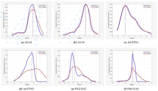
Figure 6. Distribution of classification margins for SVM vs. SSVM across six representative datasets.

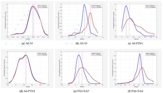
Figure 7. Distribution of classification margins for TPMSVM vs. STPMSVM across six representative datasets.

From Table 10 and Figure 6 and Figure 7, it is evident that the sparse models consistently achieve higher mean margins than their corresponding traditional models, and the peak margin values are generally larger as well. This suggests that the sparse models not only maintain better class separation but also produce more robust decision boundaries, which may help explain their improved generalization performance across different noise types.

4.2.4. Theorem Verification

In order to verify the conclusion of Theorem 1, we apply STPMSVM for the linear and nonlinear cases on Ripley’s dataset with different parameter values ($\rho ,v/\rho$)$\in \{2^{-2},2^{-1},\cdots ,2^9\}\times \{0.1,\cdots ,0.9\}$ and Gaussian kernel parameter $\gamma$ fixed at 1 for the nonlinear case. Figure 8 and Figure 9 show the relations between the parameters and the fraction of SVs and margin errors in the linear case and nonlinear case, respectively. For a clear view, we also show the relations between ${\displaystyle \frac{v}{\rho }}$ and the fraction of SVs and margin errors when $\rho =1$. It can be seen from Figure 8 and Figure 9 that the values of ${\displaystyle \frac{v}{\rho }}$ can effectively control the bounds of SVs and margin errors as pointed out by Theorem 1.

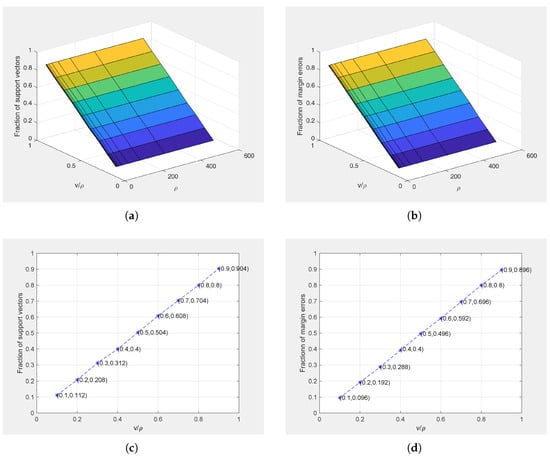
Figure 8. Relations between ($v/\rho ,\rho$) and the fractions of support vectors and margin errors on Ripley’s dataset for linear case. (a) 3D graph of the relationship between ($v/\rho ,\rho$) and the fraction of support vectors; (b) 3D graph of the relationship between ($v/\rho ,\rho$) and the fraction of margin errors; (c) Relationship between $v/\rho$ and the fraction of support vectors ($\rho =1$); (d) Relationship between $v/\rho$ and the fraction of margin errors ($\rho =1$).

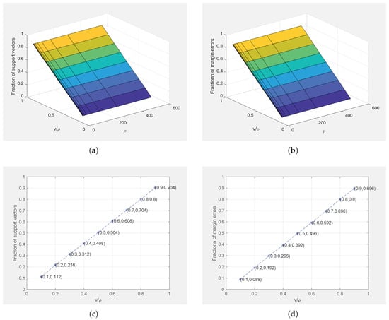
Figure 9. Relations between ($v/\rho ,\rho$) and the fractions of support vectors and margin errors on Ripley’s dataset for the non-linear case ($\gamma =1$). (a) 3D graph of the relationship between ($v/\rho ,\rho$) and the fraction of support vectors; (b) 3D graph of the relationship between ($v/\rho ,\rho$) and the fraction of margin errors; (c) Relationship between $v/\rho$ and the fraction of support vectors ($\rho =1$); (d) Relationship between $v/\rho$ and the fraction of margin errors ($\rho =1$).

4.3. Benchmark Datasets

To further test the performance of SSVM and STPMSVM, we apply the four algorithms to carry out experiments on 20 publicly available benchmark datasets (For some multi-class datasets, we take the first two classes for analysis) as follows: Balance (B1), banana (B2), bank note authentication (B3), Breast cancer (B4), cervical cancer behavior risk (B5), chemical composion of ceramic (B6), divorce predictors (B7), fertility diagnosis (B8), glass (B9), heart failure clinical records (B10), ionosphere (B11), iris (B12), movement libras (B13), Plrx (B14), seeds (B15), thyroid (B16), user knowledge modeling (B17), Wifi localization (B18), wine (B19), WDBC (B20).

The results are reported in Table 11, with learning time (the total of the training time and testing time) reported. Combined with the Wilcoxon test results, they lead to the following main findings: In terms of sparsity and efficiency, both sparse models significantly outperform their traditional counterparts. Specifically, SSVM reduces the number of support vectors by an average of 56.21% compared to SVM, while STPMSVM achieves an average reduction of 39.11% compared to TPMSVM, with STPMSVM having slightly more support vectors only on dataset B15. In terms of prediction accuracy, the differences are not statistically significant. STPMSVM achieves the highest accuracy on 12 out of 20 datasets and does not underperform TPMSVM on 18 of them. Similarly, SSVM does not underperform SVM on 13 datasets. Regarding computational cost, SSVM and STPMSVM generally require less learning time than their traditional counterparts on most datasets. The exceptions are set B3, where SSVM exhibits the longest training time. This observation aligns with our previous analysis on the impact of sample size, indicating that despite its linear objective, SSVM can still be computationally demanding for relatively large datasets.

Table 11. Results on 20 benchmark datasets.

Dataset	SVM	SSVM	TPMSVM	STPMSVM
	Acc.(%)	Acc.(%)	Acc.(%)	Acc.(%)
	Num-SVs	Num-SVs	Num-SVs	Num-SVs
	Time(s)	Time(s)	Time(s)	Time(s)
B1	99.66 ± 0.73	98.26 ± 1.15	97.23 ± 2.19	97.74 ± 1.42
(576×4)	61.20 ± 2.82	54.70 ± 2.11	369.30 ± 9.66	109.40 ± 1.17
	0.9411 ± 0.0993	0.6863 ± 0.0463	0.5706 ± 0.0662	0.5130 ± 0.0513
B2	89.25 ± 4.72	88.25 ± 4.09	89.25 ± 5.01	89.50 ± 4.97
(400×2)	93.60 ± 3.98	44.20 ± 1.55	139.40 ± 4.72	76.00 ± 12.91
	0.4390 ± 0.0306	0.3759 ± 0.0269	0.4523 ± 0.0366	0.3831 ± 0.0130
B3	99.93 ± 0.23	99.71 ± 0.38	96.50 ± 1.68	96.50 ± 1.49
(1372×4)	105.90 ± 1.60	62.60 ± 1.35	376.60 ± 1.58	132.30 ± 2.31
	2.5760 ± 0.2922	3.0472 ± 0.1801	1.7380 ± 0.1286	1.7273 ± 0.1183
B4	96.34 ± 1.58	96.49 ± 1.86	95.61 ± 2.50	96.78 ± 2.44
(683×10)	177.80 ± 2.44	44.70 ± 5.06	206.70 ± 3.20	111.50 ± 82.20
	1.1613 ± 0.1922	0.9509 ± 0.0342	0.6623 ± 0.0477	0.6107 ± 0.0114
B5	88.57 ± 11.27	90.00 ± 11.76	90.00 ± 13.55	91.43 ± 13.80
(72×19)	31.20 ± 1.48	14.20 ± 1.55	23.10 ± 2.13	15.40 ± 1.51
	0.1881 ± 0.0159	0.1558 ± 0.0171	0.3135 ± 0.0081	0.2779 ± 0.0212
B6	100.00 ± 0	100.00 ± 0	100.00 ± 0	100.00 ± 0
(88×17)	51.80 ± 1.23	24.30 ± 1.16	23.50 ± 3.10	13.50 ± 1.43
	0.2037 ± 0.0131	0.1558 ± 0.0117	0.4003 ± 0.0754	0.2913 ± 0.0157
B7	97.65 ± 5.68	97.65 ± 5.68	97.65 ± 5.68	97.65 ± 5.68
(170×54)	50.50 ± 2.51	27.10 ± 0.74	26.70 ± 2.41	17.90 ± 0.74
	0.2433 ± 0.0232	0.1826 ± 0.097	0.4075 ± 0.0280	0.3000 ± 0.0220
B8	88.00 ± 4.22	88.00 ± 4.22	74.00 ± 10.75	79.00 ± 8.76
(100×9)	33.40 ± 2.37	5.00 ± 0.83	32.40 ± 2.07	30.40 ± 2.01
	0.1947 ± 0.0185	0.1821 ± 0.0417	0.3394 ± 0.0130	0.2867 ± 0.0048
B9	67.10 ± 14.05	66.48 ± 9.12	68.57 ± 13.09	70.52 ± 10.84
(146×9)	123.90 ± 1.37	74.90 ± 2.23	124.90 ± 1.10	78.10 ± 2.81
	0.2045 ± 0.0148	0.1772 ± 0.0113	0.5731 ± 0.0216	0.2800 ± 0.0120
B10	82.57 ± 6.59	82.57 ± 6.40	80.90 ± 7.72	77.90 ± 7.85
(299×12)	138.70 ± 4.14	58.90 ± 1.97	96.50 ± 3.06	47.10 ± 4.65
	0.3627 ± 0.0296	0.2649 ± 0.0189	0.3965 ± 0.0193	0.3494 ± 0.0240
B11	94.58 ± 2.85	88.57 ± 11.27	90.00 ± 13.55	88.75 ± 13.10
(351×34)	170.70 ± 2.00	15.50 ± 1.51	23.10 ± 2.13	11.80 ± 1.03
	0.4121 ± 0.0563	0.3042 ± 0.0130	0.4648 ± 0.0270	0.3922 ± 0.0270
B12	100.00 ± 0	100.00 ± 0	100.00 ± 0	100.00 ± 0
(100×4)	43.60 ± 1.07	19.10 ± 0.57	13.00 ± 0.67	11.30 ± 0.95
	0.2200 ± 0.0378	0.1790 ± 0.0274	0.3397 ± 0.0186	0.2822 ± 0.0358
B13	85.50 ± 21.40	76.50 ± 23.10	86.00 ± 23.19	86.00 ± 23.19
(48×90)	37.40 ± 1.35	36.50 ± 1.58	43.20 ± 0.42	42.70 ± 0.48
	0.1882 ± 0.0114	0.1520 ± 0.0063	0.3543 ± 0.0204	0.2989 ± 0.0414
B14	71.46 ± 1.60	71.46 ± 1.60	73.10 ± 5.33	73.10 ± 5.33
(182×12)	120.20 ± 1.60	11.00 ± 1.54	158.60 ± 1.07	163.20 ± 0.79
	0.2580 ± 0.0333	0.1858 ± 0.0093	0.3810 ± 0.0209	0.3018 ± 0.0084
B15	94.29 ± 4.52	94.29 ± 5.63	93.57 ± 5.27	93.57 ± 4.05
(140×7)	39.80 ± 1.81	27.60 ± 0.84	16.60 ± 0.84	17.70 ± 1.34
	0.2174 ± 0.0220	0.1728 ± 0.0104	0.3379 ± 0.0166	0.2915 ± 0.0196
B16	95.35 ± 4.44	93.03 ± 4.53	94.42 ± 4.86	94.44 ± 4.81
(215×5)	27.80 ± 1.75	14.50 ± 1.35	62.20 ± 1.23	23.30 ± 1.25
	0.2548 ± 0.0170	0.2209 ± 0.0209	0.4459 ± 0.0158	0.3244 ± 0.0175
B17	100.00 ± 0	100.00 ± 0	100.00 ± 0	100.00 ± 0
(146×5)	50.80 ± 1,23	12.00 ± 1.05	61.80 ± 6.60	20.90 ± 2.38
	0.2136 ± 0.0131	0.1863 ± 0.0105	0.3505 ± 0.0108	0.2872 ± 0.0168
B18	99.90 ± 0.32	99.70 ± 0.48	99.00 ± 0.82	99.50 ± 0.53
(1000×7)	180.40 ± 2.67	81.30 ± 1.06	273.6 ± 1.35	92.50 ± 1.18
	2.0142 ± 0.2779	1.9392 ± 0.2171	1.0242 ± 0.1711	1.0186 ± 0.0257
B19	98.46 ± 3.24	98.46 ± 3.24	99.23 ± 2.43	99.92 ± 3.97
(130×13)	59.50 ± 1.72	10.80 ± 0.63	22.00 ± 1.94	17.30 ± 0.95
	0.2180 ± 0.0110	0.1819 ± 0.0125	0.3818 ± 0.0160	0.2880 ± 0.0153
B20	95.44 ± 4.23	96.84 ± 3.49	89.80 ± 4.37	96.13 ± 3.07
(569×30)	167.00 ± 3.06	38.30 ± 1.25	316.80 ± 3.22	57.30 ± 1.49
	0.8059 ± 0.1276	0.5963 ± 0.0114	0.5166 ± 0.0571	0.4895 ± 0.0165
Avg. SV-Reduction (%)	—	56.21	—	39.11
p-value/r (Acc.)	a 0.1279/0.3404	c 0.5349/0.1387	b 0.1055/0.3620
p-value/r (Num-SVs)	a,* 0.0001/0.8765 (SSVM < SVM)	c,* 0.0479/0.4424 (SSVM < STPMSVM)	b,* 0.0003/0.8181 (STPMSVM < TPMSVM)
p-value/r (Time)	a,* 0.0015/0.7096 (SSVM < SVM)	c 0.4330/0.1753	b,* 0.0001/0.8765 (STPMSVM < TPMSVM)

These results indicate that although SSVM employs a linear objective, its training can still be time—consuming on relatively large datasets. In practice, for smaller datasets where prediction speed is critical, SSVM remains a viable option, despite its generally lower accuracy than STPMSVM under noisy conditions. In contrast, STPMSVM not only provides sparse solutions and reduced computational complexity but also maintains—and in many cases enhances—generalization performance, making it the more robust and effective choice overall.

Beyond the above quantitative metrics, the experimental outcomes in this paper provide profound insights into the underlying mechanism. The collective results consistently demonstrate that the proposed SSVM and STPMSVM models achieve a significant reduction in the number of SVs compared to their standard counterparts. This pervasive phenomenon provides strong empirical validation that the initial geometric motivation of employing an ${\ell }_1$-norm penalty—to break rotational symmetry—has been successfully translated, via the KKT conditions, into the final models’ operational principle. The resulting sparsity of the solutions stands as direct empirical evidence for the successful implementation of the initial symmetry-breaking design.

5. Conclusions and Future Work

In this paper, we present two novel sparse models, SSVM and STPMSVM, which achieve high sparsity and computational efficiency benefits from the LPPs by fundamentally rethinking the regularization geometry. In the SSVM model, a pair of parallel hyperplanes, similar to those in SVM, is constructed, while in the STPMSVM model, a pair of non-parallel hyperplanes is obtained, following the spirit of TPMSVM. The core of our approach lies in a symmetry-breaking design: we replace the rotationally symmetric ${\ell }_2$-norm with the axis-aligned ${\ell }_1$-norm on the dual variables to induce sparsity. This explicit geometric motivation is then structurally transformed via the KKT conditions. The ${\ell }_1$-norm penalty is absorbed into the model’s framework, emerging as a linear term in SSVM or reduced to a constant (and thereby vanishing) in STPMSVM. This key transformation allows the original QPPs to be reformulated as more efficient LPPs. Consequently, sparsity is no longer an explicitly penalized term but an implicitly enforced property of the solution, governed by the problem constraints and the geometry of linear programming. Numerical experiments on synthetic and benchmark datasets confirm the efficacy of this paradigm. Both models achieve superior sparsity and faster prediction speeds. Specifically, SSVM excels in producing the sparsest solutions, while STPMSVM robustly combines high accuracy with strong sparsity, inheriting the benefits of the TPMSVM architecture.

Despite these advantages, we note that several limitations remain in this study. The proposed models currently rely on kernel computations for nonlinear cases, which may limit scalability to very large datasets, though they are suitable for real-time prediction in edge computing scenarios. Potential solution: degeneracy can occur due to linear programming vertex solutions. In addition, comparisons with other sparse models are limited in this study.

Future work includes extending SSVM/STPMSVM to multiclass, online/streaming, or structured-output settings; integrating low-rank kernel approximations (e.g., Nyström, random features) for scalable large-scale training, developing more efficient and accurate hyperparameter tuning strategies, and exploring comparisons with additional sparse approaches to provide a more comprehensive evaluation and further investigate sparsity and generalization performance.

References

- Shalev-Shwartz, S.; Ben-David, S. Understanding Machine Learning: From Theory to Algorithms; Cambridge University Press: Cambridge, UK, 2014. [Google Scholar]
- Cortes, C.; Vapnik, V. Support-vector networks. Mach. Learn. 1995, 20, 273–297. [Google Scholar] [CrossRef]
- Schölkopf, B.; Smola, A.J. Learning with Kernels: Support Vector Machines, Regularization, Optimization, and Beyond; MIT Press: Cambridge, MA, USA, 2002. [Google Scholar]
- Shawe-Taylor, J.; Cristianini, N. Kernel Methods for Pattern Analysis; Cambridge University Press: Cambridge, UK, 2004. [Google Scholar]
- Vapnik, V.N. An overview of statistical learning theory. IEEE Trans. Neural Netw. 1999, 10, 988–999. [Google Scholar] [CrossRef]
- Cervantes, J.; Garcia-Lamont, F.; Rodríguez-Mazahua, L.; Lopez, A. A comprehensive survey on support vector machine classification: Applications, challenges and trends. Neurocomputing 2020, 408, 189–215. [Google Scholar] [CrossRef]
- Hao, P.Y. New support vector algorithms with parametric insensitive/margin model. Neural Netw. 2010, 23, 60–73. [Google Scholar] [CrossRef] [PubMed]
- Khemchandani, R.; Jayadeva; Chandra, S. Twin support vector machines for pattern classification. IEEE Trans. Pattern Anal. Mach. Intell. 2007, 29, 905–910. [Google Scholar] [CrossRef]
- Peng, X. TPMSVM: A novel twin parametric-margin support vector machine for pattern recognition. Pattern Recognit. 2011, 44, 2678–2692. [Google Scholar] [CrossRef]
- Tanveer, M.; Rajani, T.; Rastogi, R.; Shao, Y.H.; Ganaie, M.A. Comprehensive review on twin support vector machines. Ann. Oper. Res. 2024, 339, 1223–1268. [Google Scholar] [CrossRef]
- Li, Y.; Zhao, L. Application of support vector machine algorithm in predicting the career development path of college students. Int. J. High Speed Electron. Syst. 2025, 2540230. [Google Scholar] [CrossRef]
- Chandra, M.A.; Bedi, S.S. Survey on SVM and their application in image classification. Int. J. Inf. Technol. 2021, 13, 1–11. [Google Scholar] [CrossRef]
- Zeng, S.; Chen, M.; Li, X.; Wu, Y. A financial distress prediction model based on sparse algorithm and support vector machine. Math. Probl. Eng. 2020, 2020, 5625271. [Google Scholar] [CrossRef]
- Madhu, B.; Rakesh, A.; Rao, K.S. A comparative study of support vector machine and artificial neural network for option price prediction. J. Comput. Commun. 2021, 9, 78–91. [Google Scholar] [CrossRef]
- Kok, Z.H.; Chua, L.S.; Aziz, N.A.; Ismail, W.I.W. Support vector machine in precision agriculture: A review. Comput. Electron. Agric. 2021, 191, 106546. [Google Scholar] [CrossRef]
- Abdullah, D.M.; Abdulazeez, A.M. Machine learning applications based on SVM classification: A review. Qubahan Acad. J. 2021, 1, 81–90. [Google Scholar] [CrossRef]
- Malashin, I.; Tynchenko, V.; Gantimurov, A.; Nelyub, V.; Borodulin, A. Support vector machines in polymer science: A review. Polymers 2025, 17, 491. [Google Scholar] [CrossRef]
- Khyathi, G.; Indumathi, K.P.; Jumana Hasin, A.; Lisa Flavin Jency, M.; Krishnaprakash, G.; Lisa, F.J.M. Support vector machines: A literature review on their application in analyzing mass data for public health. Cureus 2025, 17, e000000. [Google Scholar] [CrossRef]
- Yang, L.; Dong, H. Support vector machine with truncated pinball loss and its application in pattern recognition. Chemom. Intell. Lab. Syst. 2018, 177, 89–99. [Google Scholar] [CrossRef]
- De Leone, R.; Maggioni, F.; Spinelli, A. A multiclass robust twin parametric margin support vector machine with an application to vehicles emissions. In Proceedings of the International Conference on Machine Learning, Optimization, and Data Science, Grasmere, UK, 22–26 September 2023; Springer Nature: Cham, Switzerland, 2023; pp. 299–310. [Google Scholar]
- Wang, H.; Shao, Y. Fast truncated Huber loss SVM for large-scale classification. Knowl.-Based Syst. 2023, 260, 110074. [Google Scholar] [CrossRef]
- Wang, H.; Zhang, H.; Li, W. Sparse and robust support vector machine with capped squared loss for large-scale pattern classification. Pattern Recognit. 2024, 153, 110544. [Google Scholar] [CrossRef]
- Sui, Y.; He, X.; Bai, Y. Implicit regularization in over-parameterized support vector machine. Adv. Neural Inf. Process. Syst. 2023, 36, 31943–31966. [Google Scholar]
- Moosaei, H.; Hladík, M. Sparse solution of least-squares twin multi-class support vector machine using ℓ0 and ℓp-norm for classification and feature selection. Neural Netw. 2023, 166, 471–486. [Google Scholar] [CrossRef]
- Tang, Q.; Li, G. Sparse L0-norm least squares support vector machine with feature selection. Inf. Sci. 2024, 670, 120591. [Google Scholar] [CrossRef]
- Li, N.; Zhang, H.H. Sparse learning with non-convex penalty in multi-classification. J. Data Sci. 2021, 19, 1–20. [Google Scholar] [CrossRef]
- Zhou, S. Sparse SVM for sufficient data reduction. IEEE Trans. Pattern Anal. Mach. Intell. 2021, 44, 5560–5571. [Google Scholar] [CrossRef] [PubMed]
- Lu, S.; Li, Q. A majorization penalty method for SVM with sparse constraint. Optim. Methods Softw. 2023, 38, 474–494. [Google Scholar] [CrossRef]
- Zhu, J.; Rosset, S.; Hastie, T.; Tibshirani, R. 1-norm support vector machines. Adv. Neural Inf. Process. Syst. 2003, 16. [Google Scholar]
- Qu, S.; De Leone, R.; Huang, M. Sparse learning for linear twin parameter-margin support vector machine. In Proceedings of the 3rd Asia Conference on Algorithms, Computing and Machine Learning, Shanghai, China, 22–24 March 2024; pp. 50–55. [Google Scholar]
- Qu, S.; Huang, M.; De Leone, R.; Maggioni, F.; Spinelli, A. An efficient sparse twin parametric insensitive support vector regression model. Mathematics 2025, 13, 2206. [Google Scholar] [CrossRef]
- Wolfe, P. A duality theorem for non-linear programming. Q. Appl. Math. 1961, 19, 239–244. [Google Scholar] [CrossRef]
Disclaimer/Publisher’s Note: The statements, opinions and data contained in all publications are solely those of the individual author(s) and contributor(s) and not of MDPI and/or the editor(s). MDPI and/or the editor(s) disclaim responsibility for any injury to people or property resulting from any ideas, methods, instructions or products referred to in the content. |
© 2025 by the authors. Licensee MDPI, Basel, Switzerland. This article is an open access article distributed under the terms and conditions of the Creative Commons Attribution (CC BY) license (https://creativecommons.org/licenses/by/4.0/).