Modified Fokas–Lenells Equation: Self-Consistent Sources and Soliton Solutions of the Spin and (2+1)-Dimensional Models

Abstract

Nonlinear evolution equations play a key role in modeling various physical processes, such as wave propagation in nonlinear optical and hydrodynamic media, as well as in the dynamics of plasma and quantum systems. In this paper, we study an integrable generalization of the nonlinear Schrödinger equation: the Fokas–Lenells (FL) equation. We derive a new (1+1)-dimensional FL equation with self-consistent sources, which enables modeling the interaction of solitons with external disturbances within the framework of integrable systems. For the frist time, we obtain, two distinct types of solutions for the spin system of the FL equation, namely, a traveling wave and a one-soliton solution, derived using the Darboux transformation (DT). We also construct exact one-soliton and two-soliton solutions for the (2+1)-dimensional FL equation using the DT. These results advance analytical methods in the theory of integrable nonlinear systems, including spin models widely used to describe magnetic, quantum, and soliton phenomena. We illustrate the dynamics of the solutions graphically.

1. Introduction

Nowadays, there is great interest in the study of nonlinear differential equations, since many physical phenomena in nature are nonlinear and require nonlinear equations for their accurate description. Thus, integrable nonlinear equations hold a prominent position in the theory of nonlinear waves, integrable systems, and mathematical physics. They serve not only as precise models for complex physical processes but also as a basis for constructing exact analytical solutions using advanced mathematical techniques [1,2,3].

To obtain such solutions, researchers have developed a range of powerful methods, including the Hirota bilinear approach [4,5], the sine-cosine method [6], the Darboux transformation (DT) [7,8,9], and the hyperbolic tangent technique [10,11]. These tools are essential in uncovering the rich mathematical structure and solution space of integrable systems.

One notable example of an integrable equation is the Fokas–Lenells (FL) equation, which was originally derived via the bi-Hamiltonian approach and introduced by Fokas in 1995 [12]. The Lax representation (LR) of the FL equation was later developed by Fokas and Lenells in 2009 [13,14,15,16]. The FL equation models the propagation of ultrashort optical pulses in nonlinear media and acts as an integrable generalization of the nonlinear Schrödinger equation (NLSE), incorporating higher-order dispersion and nonlinear effects [17,18].

In the (1+1)-dimensional formulation, the FL equation is given by

$$i{q}_{xt}-i{q}_{xx}+2q_x-{|q|}^2{q}_x+iq=0,$$

(1)

where q represents the complex envelope of the field; the subscripts x and t denote partial derivatives with respect to the corresponding variables, and i is the imaginary unit.

The equation also exhibits a rich solution structure, which has attracted considerable attention from researchers and has led to numerous significant results [19], including various classes of exact solutions. These include rogue wave solutions [20], bright [21] and dark soliton solutions [22], multisoliton solutions constructed via the Darboux transformation (DT) [23], as well as exact solutions corresponding to nonlocal generalizations of the equation [24].

One of the key directions in the advancement of integrable models is the integration of self-consistent sources. This approach has been actively explored across a wide range of physical contexts [25,26,27]. For instance, the NLSE with self-consistent sources captures the interaction between ion-acoustic waves in a two-component plasma and high-frequency electrostatic oscillations [28,29]. A similar generalization of Equation (1) can be obtained by introducing self-consistent sources, which allows for modeling the coupling between nonlinear wave fields and external potentials or supplementary dynamic excitations. Moreover, the pursuit of novel integrable systems that admit N-soliton solutions continues to be a vibrant and challenging area within the contemporary theory of integrable systems [30,31].

In addition, spin systems associated with integrable equations have attracted considerable interest [32]. One of the earliest and most significant spin models is the Heisenberg ferromagnet, which serves as a generalization of the Landau-Lifshitz (LL) equation. The LL equation is known to be gauge equivalent to the nonlinear Schrödinger equation (NLSE) [33,34,35]. Another notable example is the spin system of the integrable FL equation (FLSS) [36].

There is also growing interest in the study of multidimensional integrable systems due to their rich internal structure and broad applicability in nonlinear science and mathematical physics [37]. It is worth noting that the FL equation exhibits strong nonlinearity and admits Lax pairs that differ significantly from those of the classical AKNS hierarchy. This poses significant analytical challenges in deriving exact solutions, especially in higher dimensions, thereby motivating the investigation of the (2+1)-dimensional generalization of the FL equation.

The study of the (2+1)-dimensional FL equation has attracted considerable attention in recent years. In [38], the nonlinear dynamical behavior of higher-order rogue wave solutions was analyzed, while in [39], various wave-interaction phenomena—such as solitons, degenerate solitons, lumps, and lump chains—were explored. Moreover, in [40], a parameterized version of the (2+1)-dimensional FL equation was investigated using a combination of Wronskian and bilinear techniques.

All these aspects—from the classical (1+1)-dimensional model and its extension with a self-consistent source to the (2+1)-dimensional generalizations and the corresponding spin model—highlight the diversity and richness of structures emerging within the theory of integrable systems. Their investigation not only deepens our understanding of the mathematical properties of the underlying equations but also facilitates the modeling and interpretation of physical processes in complex media.

In this paper, we further develop these directions by focusing on three interrelated problems. First, we propose a (1+1)-dimensional FL equation with self-consistent sources (FLESCS) along with its associated Lax pair. Second, we develop novel classes of exact solutions for the spin system that emerges as a gauge-equivalent counterpart of the FL equation, including a one-soliton solution constructed via the DT and a traveling wave solution obtained through angular parametrization of the spin vector, both subjected to a comprehensive analytical and dynamical characterization. Third, we derive exact one- and two-soliton solutions of the (2+1)-dimensional FL equation using a generalized DT.

The choice of the DT among other well-known methods is motivated by its proven effectiveness and versatility in constructing exact solutions for integrable systems. In comparison with other analytical approaches, such as the Hirota bilinear method, the Riemann-Hilbert approach, the inverse scattering transform, and the Bäcklund transformation, the DT offers a more direct and algebraically constructive framework for generating explicit solutions. While the Hirota method requires bilinearization and perturbative expansions, and the Riemann–Hilbert and inverse scattering techniques rely on complex spectral analysis, the DT provides a systematic way to derive higher-order soliton solutions from a simple seed solution. Although conceptually related to the Bäcklund transformation, the DT has a distinct advantage in being naturally formulated through the Lax pair representation, which simplifies the construction of matrix and vector generalizations. This makes the DT particularly efficient for equations with intricate Lax pair structures, such as the FL equation. Moreover, the DT facilitates the construction of more complex localized structures—such as rogue waves and breathers—thereby extending the class of solutions. Finally, we explore the physical interpretation of the obtained solutions and the interconnections among the various models under consideration. These contributions not only broaden the spectrum of known integrable models but also highlight the effectiveness of the DT in addressing multidimensional and spin-type integrable systems.

Section 2 introduces the (1+1)-dimensional FLESCS and presents various solutions of the FLSS. Section 3 is devoted to the construction of one-fold and two-fold DT for the (2+1)-dimensional FL equation, which are then used to derive exact one- and two-soliton solutions. Finally, Section 4 summarizes the main conclusions of the study.

2. Integrable Models Associated with the (1+1)-Dimensional FL Equation

This section is devoted to integrable models related to the (1+1)-dimensional FL equation. We begin with the derivation of the FLESCS equation—an extension of the FL equation that incorporates self-consistent sources. This model describes an important type of nonlinear system that helps explain how wave fields interact with external forces.

Next, we examine the solution spin system of the FL equation, which serves as a prominent example of an integrable model arising from a distinct area of physics—namely, the theory of spin systems. The spin system of the FL equation is a gauge-equivalent model of the FL equation, but considered in the context of spin dynamics. This equation describes the interactions of spin fields in various materials and systems, which is critically important for understanding magnetic and quantum phenomena.

2.1. The (1+1)-Dimensional FLESCS

This section introduces a novel integrable model, the FLESCS, which can be expressed in the following form:

$$i{q}_{xt}-i{q}_{xx}+2q_x-{\left|q\right|}^2{q}_x+iq+p=0.$$

(2)

The source expression under consideration corresponds to the spectral problem associated with the FL equation. Equation (2) can be rewritten in a modified form for $r=q^{*}$, while choosing $r=-q^{*}$ leads to Equation (2) with a change in the sign of the nonlinear term

$$\begin{array}{c}\hfill i{q}_{xt}-i{q}_{xx}+2q_x-q_{x}qr+iq+p=0,\end{array}$$

(3)

$$\begin{array}{c}\hfill i{r}_{xt}-i{r}_{xx}-2r_x+r_{x}rq+ir+k=0.\end{array}$$

(4)

Here, p and k are unknown functions to be determined.

The Lax pair corresponding to Equations (3) and (4) is given by

$$\begin{array}{ccc}\hfill {\Psi }_x& =& U\Psi ,\hfill \\ \hfill {\Psi }_t& =& V\Psi ,\hfill \end{array}$$

where $\Psi \left(\lambda \right)$ is the eigenfunction associated with the spectral parameter $\lambda$, and the operators U and V are matrix operators of the form

$$\begin{array}{ccc}\hfill U& =& -i{\lambda }^2{\sigma }_3+\lambda Q,\hfill \\ \hfill V& =& U+B_0+{\displaystyle \frac{1}{\lambda }}{B}_{-1}+{\displaystyle \frac{1}{{\lambda }^2}}{B}_{-2}+{\displaystyle \frac{\mu }{\lambda +\eta }}{C}_{-1},\hfill \end{array}$$

Here,

$$Q=\left(\begin{array}{cc}0& q_x\\ r_x& 0\end{array}\right),{\sigma }_3=\left(\begin{array}{cc}1& 0\\ 0& -1\end{array}\right),B_0=\left(a_{ij}\right),B_{-1}=\left(b_{ij}\right),B_{-2}=\left(c_{ij}\right),C_{-1}=\left(n_{ij}\right),$$

with $a_{ij}$, $b_{ij}$, $c_{ij}$, and $n_{ij}$$(i,j=1,2)$ being unknown matrix elements to be determined, and $\mu$ and $\eta$ are real constants. Consider the compatibility condition ${\Psi }_{xt}={\Psi }_{tx}$ in powers of $\lambda$, namely,

$$\begin{array}{ccc}\hfill {\lambda }^2:& & -[{\sigma }_3,B_0]=0,\hfill \end{array}$$

(5)

$$\begin{array}{ccc}\hfill {\lambda }^1:& & Q_t-Q_x+[Q,B_0]-i[{\sigma }_3,B_{-1}]-i\mu [{\sigma }_3,C_{-1}]=0,\hfill \end{array}$$

(6)

$$\begin{array}{ccc}\hfill {\lambda }^0:& & -B_{0x}+[Q,B_{-1}]-i[{\sigma }_3,B_{-2}]+i\mu \eta [{\sigma }_3,C_{-1}]+\mu [Q,C_{-1}]=0,\hfill \end{array}$$

(7)

$$\begin{array}{ccc}\hfill {\lambda }^{-1}:& & -B_{-1x}+[Q,B_{-2}]=0,\hfill \end{array}$$

(8)

$$\begin{array}{ccc}\hfill {\lambda }^{-2}:& & -B_{-2x}=0,\hfill \end{array}$$

(9)

$$\begin{array}{ccc}\hfill -{\displaystyle \frac{\mu }{\lambda +\eta }}:& & C_{-1x}+i{\eta }^2[{\sigma }_3,C_{-1}]+\eta [Q,C_{-1}]=0.\hfill \end{array}$$

(10)

From Equation (5), it follows that:

$$a_{12}=0,$$

$$a_{21}=0,$$

and from Equation (6) we obtain

$$q_x{a}_{21}=a_{12}{r}_x,$$

$$q_x{a}_{21}=a_{12}{r}_x,$$

$$q_{xt}-q_{xx}-q_x{a}_{1122}-2i{b}_{12}-2i\mu n_{12}=0,$$

$$r_{xt}-r_{xx}-r_x{a}_{1122}+2i{b}_{21}+2i\mu n_{21}=0,$$

For convenience, we introduce the following notations:

$$a_{1122}=a_{11}-a_{22},n_{1122}=n_{11}-n_{22},c_{1122}=c_{11}-c_{22}.$$

Equation (7) yields

$$\begin{array}{ccc}\hfill a_{11x}& =& q_x{b}_{21}-r_x{b}_{12}+\mu (r_x{n}_{12}-q_x{n}_{21}),\hfill \end{array}$$

(11)

$$\begin{array}{ccc}\hfill a_{22x}& =& -q_x{b}_{21}+r_x{b}_{12}-\mu (r_x{n}_{12}-q_x{n}_{21}),\hfill \end{array}$$

(12)

$$\begin{array}{ccc}\hfill a_{21x}& =& r_x{b}_{1122}+2i{c}_{21}-2i\mu \eta n_{21}+\mu r_x{n}_{1122},\hfill \end{array}$$

(13)

$$\begin{array}{ccc}\hfill a_{12x}& =& -q_x{b}_{1122}-2i{c}_{12}+2i\mu \eta n_{12}-\mu q_x{n}_{1122},\hfill \end{array}$$

(14)

From Equations (11) and (12) we obtain

$$a_{11x}=-a_{22x},a_{11}=-a_{22},$$

and Equation (9) gives

$$c_{11x}=c_{12x}=c_{21x}=c_{22x}=0,c_{ij}=\mathrm{const}.$$

(15)

Taking into account Equation (15), from Equation (8) we find

$$\begin{array}{ccc}\hfill b_{11x}& =& q_x{c}_{21}-r_x{c}_{12},b_{11}=q{c}_{21}-r{c}_{12},\hfill \end{array}$$

(16)

$$\begin{array}{ccc}\hfill b_{22x}& =& -(q_x{c}_{21}-r_x{c}_{12}),b_{22}=-b_{11},\hfill \end{array}$$

(17)

$$\begin{array}{ccc}\hfill b_{12x}& =& -q_x{c}_{1122},b_{12}=-q{c}_{1122},\hfill \end{array}$$

(18)

$$\begin{array}{ccc}\hfill b_{21x}& =& r_x{c}_{1122},b_{21}=r{c}_{1122},\hfill \end{array}$$

(19)

from Equation (10) we have

$$n_{11x}=\eta (r_x{n}_{12}-q_x{n}_{21}),$$

(20)

$$n_{22x}=-\eta (r_x{n}_{12}-q_x{n}_{21}),$$

(21)

$$n_{11x}=-n_{22x},n_{11}=-n_{22},$$

(22)

$$n_{12x}+2i{\eta }^2{n}_{12}-2\eta q_x{n}_{11}=0,$$

(23)

$$n_{21x}-2i{\eta }^2{n}_{21}+2\eta r_x{n}_{11}=0.$$

(24)

Applying Equations (20) and (22) to Equations (11) and (12), we obtain

$$\begin{array}{ccc}\hfill a_{11}& =& qr{c}_{1122}-{\displaystyle \frac{\mu }{\eta }}{n}_{22}+a_{110},\hfill \end{array}$$

(25)

$$\begin{array}{ccc}\hfill a_{22}& =& -qr{c}_{1122}+{\displaystyle \frac{\mu }{\eta }}{n}_{22}+a_{220},\hfill \end{array}$$

(26)

Substituting Equations (13) and (14) into Equations (23) and (24), respectively, we get

$$\begin{array}{ccc}\hfill n_{12x}& =& 0,\hfill \\ \hfill n_{21x}& =& 0.\hfill \end{array}$$

Integrating Equations (20) and (21), we find

$$\begin{array}{ccc}\hfill n_{11}& =& \eta r{n}_{12}-\eta q{n}_{21}+n_{110},\hfill \\ \hfill n_{22}& =& -\eta r{n}_{12}+\eta q{n}_{21}+n_{220},\hfill \end{array}$$

where $a_{110}$, $a_{220}$, $n_{110}$, and $n_{220}$ are constants of integration.

Assume that the constants take the following values:

$$c_{11}=-{\displaystyle \frac{i}{4}},c_{22}={\displaystyle \frac{i}{4}},c_{12}=0,c_{21}=0,n_{12}=0,n_{21}=0,n_{11}=i,n_{22}=-i.$$

Then, Equations (16)–(19) become

$$b_{11}=0,b_{22}=0,b_{12}={\displaystyle \frac{iq}{2}},b_{21}=-{\displaystyle \frac{ir}{2}},$$

and Equations (25) and (26) take the form

$$a_{11}=-{\displaystyle \frac{iqr}{2}}+i+i{\displaystyle \frac{\mu }{\eta }},a_{22}={\displaystyle \frac{iqr}{2}}-i-i{\displaystyle \frac{\mu }{\eta }},$$

as well as

$$n_{11}=i,n_{22}=-i.$$

Thus,

$$B_0=i{\sigma }_3-{\displaystyle \frac{iqr}{2}}{\sigma }_3+i\left(\begin{array}{cc}{\displaystyle \frac{\mu }{\eta }}& 0\\ 0& -{\displaystyle \frac{\mu }{\eta }}\end{array}\right),B_{-1}={\displaystyle \frac{i}{2}}\left(\begin{array}{cc}0& q\\ -r& 0\end{array}\right),B_{-2}={\displaystyle \frac{i}{4}}{\sigma }_3,C_{-1}=i{\sigma }_3.$$

Thus, Equations (3) and (4) take the following form:

$$\begin{array}{c}\hfill i{q}_{xt}-i{q}_{xx}+2q_x-qr{q}_x+iq+{\displaystyle \frac{2\mu }{\eta }}{q}_x=0,\end{array}$$

(27)

$$\begin{array}{c}\hfill i{r}_{xt}-i{r}_{xx}-2r_x+r_{x}rq+ir-{\displaystyle \frac{2\mu }{\eta }}{r}_x=0.\end{array}$$

(28)

Hence, Equations (27) and (28) represent the desired FLESCS system. The opposite signs in the linear derivative terms of Equations (27) and (28) reflect the conjugate nature of the fields q and r, corresponding to solitons of opposite polarity.

Moreover, for Equations (27) and (28), the matrix operators U and V take the form

$$\begin{array}{ccc}\hfill U& =& -i{\lambda }^2{\sigma }_3+\lambda Q,\hfill \\ \hfill V& =& U+V_0+{\displaystyle \frac{1}{\lambda }}{V}_{-1}-{\displaystyle \frac{i}{4{\lambda }^2}}{\sigma }_3+iM+i{\displaystyle \frac{\mu }{\lambda +\eta }}{\sigma }_3,\hfill \end{array}$$

where

$$V_0=i{\sigma }_3-{\displaystyle \frac{iqr}{2}}{\sigma }_3,V_{-1}={\displaystyle \frac{i}{2}}\left(\begin{array}{cc}0& q\\ -r& 0\end{array}\right),M=\left(\begin{array}{cc}{\displaystyle \frac{\mu }{\eta }}& 0\\ 0& -{\displaystyle \frac{\mu }{\eta }}\end{array}\right).$$

2.2. The FLSS

Matrix form of FLSS is given by [36]

$$i{A}_t+{\displaystyle \frac{b}{2}}[A,A_{xx}-A_{xt}]+i(b^2-1)A_x=0,$$

(29)

where $A=A(x,t)$ is a $2\times 2$ matrix describing the spin variable, $b={\displaystyle \frac{1}{2{\lambda }_0^2}}$ with ${\lambda }_0$ an arbitrary constant. Square brackets denote the matrix commutator. The matrix A is expressed via the components of the spin vector $\mathbf{A}=(A_1,A_2,A_3)$ as

$$A=\left(\begin{array}{cc}{A}_3& A^{-}\\ A^{+}& -A_3\end{array}\right),A^2=I,A^{\pm }=A_1\pm i{A}_2,$$

where I is the identity matrix and the condition $A^2=I$ reflects the normalization ${\parallel \mathbf{A}\parallel }^2=1$. Such a structure is typical for algebraic representations of $\mathfrak{su}\left(2\right)$ and is essential for preserving the unitarity of gauge transformations.

The integrability of the FLSS is guaranteed by the existence of a Lax pair

$$\begin{array}{cc}\hfill {\Phi }_x& =U_1\Phi ,\hfill \end{array}$$

(30)

$$\begin{array}{cc}\hfill {\Phi }_t& =V_1\Phi ,\hfill \end{array}$$

(31)

where $\Phi ={({\Phi }_1,{\Phi }_2)}^T$ is the eigenfunction, and the matrices $U_1$ and $V_1$ depend on the spectral parameter $\lambda$ and are explicitly given by

$$U_1=-i({\lambda }^2-{\lambda }_0^2)A+{\displaystyle \frac{(\lambda -{\lambda }_0)}{2{\lambda }_0}}A{A}_x,$$

(32)

$$V_1=-i\left({\lambda }^2-{\lambda }_0^2+{\displaystyle \frac{1}{4{\lambda }^2}}-{\displaystyle \frac{1}{4{\lambda }_0^2}}\right)A+\left({\displaystyle \frac{\lambda }{2{\lambda }_0}}-{\displaystyle \frac{{\lambda }_0}{2\lambda }}\right)A{A}_x+\left({\displaystyle \frac{{\lambda }_0}{2\lambda }}-{\displaystyle \frac{1}{2}}\right)A{A}_t.$$

(33)

The connection between the FLSS and the FL equation is established through the gauge transformation

$$\Phi =g^{-1}{\Psi ,g=\Psi |}_{\lambda ={\lambda }_0},$$

(34)

where $\Psi$ is a solution to the Lax pair of the FL equation, and $g(x,t)$ is a unitary gauge transformation matrix. The Lax pair for the FL equation is given by

$$\begin{array}{cc}\hfill {\Psi }_x& =U(x,t,\lambda )\Psi ,\hfill \end{array}$$

(35)

$$\begin{array}{cc}\hfill {\Psi }_t& =V(x,t,\lambda )\Psi .\hfill \end{array}$$

(36)

The matrix g satisfies the system

$$g_x=U_{0}g,U_0(x,t)=-i{\lambda }_0^2{\sigma }_3+{\lambda }_{0}Q(x,t),$$

$$g_t=Fg,F(x,t)=-i{\lambda }_0^2{\sigma }_3+{\lambda }_{0}Q+V_0+{\displaystyle \frac{1}{{\lambda }_0}}{V}_{-1}-{\displaystyle \frac{i}{4{\lambda }_0^2}}{\sigma }_3,$$

which corresponds to the zero curvature condition $U_{0t}-F_x+[U_0,F]=0$.

Substituting the gauge transformation $A=g^{-1}{\sigma }_{3}g$ and using the expressions for U and V, we obtain the transformed equations

$${\Phi }_x=\left(-i({\lambda }^2-{\lambda }_0^2)g^{-1}{\sigma }_{3}g+(\lambda -{\lambda }_0)g^{-1}Qg\right)\Phi ,$$

$${\Phi }_t=\left(-i({\lambda }^2-{\lambda }_0^2)g^{-1}{\sigma }_{3}g+(\lambda -{\lambda }_0)g^{-1}Qg+\left({\displaystyle \frac{1}{\lambda }}-{\displaystyle \frac{1}{{\lambda }_0}}\right)g^{-1}{V}_{-1}g-{\displaystyle \frac{i}{4}}\left({\displaystyle \frac{1}{{\lambda }^2}}-{\displaystyle \frac{1}{{\lambda }_0^2}}\right)g^{-1}{\sigma }_{3}g\right)\Phi .$$

Thus, the FLSS can be derived from the FL equation by means of this gauge transformation, confirming their integrability and structural equivalence. This relationship allows the application of integral geometry and scattering theory techniques to the analysis of spin systems.

The following subsection is devoted to constructing exact analytical solutions of the FLSS.

2.3. Traveling Wave Solutions of the FLSS

Traveling wave solutions are those that propagate with a constant velocity while preserving their shape. They play a crucial role in various scientific fields, including nonlinear optics, spin media, and magnetism.

Let us consider the angular parametrization of the spin vector [36]

$$A^{+}=\sin \theta e^{i\phi },A^{-}=\sin \theta e^{-i\phi },A_3=\cos \theta ,$$

(37)

where $\theta (x,t)$ and $\phi (x,t)$ are real-valued functions characterizing the orientation of the spin vector on the unit sphere.

Substituting this parametrization into the matrix form of the FLSS yields an equivalent system in terms of the components $A_3$, $A^{+}$, and $A^{-}$,

$$\begin{array}{ccc}\hfill i{A}_{3t}& =& {\displaystyle \frac{b}{2}}(A^{-}{A}_{xt}^{+}-A^{-}{A}_{xx}^{+}+A_{xx}^{-}{A}^{+}-A_{xt}^{-}{A}^{+})-i(b^2-1)A_{3x},\hfill \end{array}$$

(38)

$$\begin{array}{ccc}\hfill i{A}_t^{+}& =& b(A^{+}{A}_{3xt}-A^{+}{A}_{3xx}+A_3{A}_{xx}^{+}-A_3{A}_{xt}^{+})-i(b^2-1)A_x^{+},\hfill \end{array}$$

(39)

$$\begin{array}{ccc}\hfill i{A}_t^{-}& =& b(A^{-}{A}_{3xx}-A^{-}{A}_{3xt}-A_3{A}_{xx}^{-}+A_3{A}_{xt}^{-})-i(b^2-1)A_x^{-},\hfill \end{array}$$

(40)

where $b=1/\left(2{\lambda }_0^2\right)$.

By switching to angular variables and applying algebraic transformations, we obtain the following system of equations:

$${\theta }_t=b\left({\phi }_{xx}\sin \theta +2{\phi }_x{\theta }_x\cos \theta -{\phi }_{xt}\sin \theta -{\phi }_x{\theta }_t\cos \theta -{\theta }_x{\phi }_t\cos \theta \right)-(b^2-1){\theta }_x,$$

(41)

$${\phi }_t=b\left({\displaystyle \frac{{\theta }_{xt}}{\sin \theta }}-{\displaystyle \frac{{\theta }_{xx}}{\sin \theta }}+{\phi }_x^2\cos \theta -{\phi }_x{\phi }_t\cos \theta \right)-(b^2-1){\phi }_x.$$

(42)

It is assumed that the desired solutions of a traveling wave depend on the following combination:

$$\xi =x-vt.$$

(43)

where v is the wave propagation velocity.

Taking into account Equation (43), we rewrite Equation (41) as follows:

$$-v{\theta }^{\prime }=b\left({\phi }^{″}\sin \theta +2{\phi }^{\prime }{\theta }^{\prime }\cos \theta +v{\phi }^{″}\sin \theta +v{\phi }^{\prime }{\theta }^{\prime }\cos \theta +v{\theta }^{\prime }{\phi }^{\prime }\cos \theta \right)-(b^2-1){\theta }^{\prime }.$$

(44)

Similarly, from Equation (42) we derive

$${\phi }^{\prime }={\displaystyle \frac{a\cos \theta -C_1}{(1+v){\sin }^2\theta }},$$

(45)

where $a={\displaystyle \frac{1-b^2+v}{b}}$ and $C_1$ is an arbitrary constant.

Introducing the substitution $\omega =\cos \theta$, Equation (45) becomes

$${\phi }^{\prime }={\displaystyle \frac{a\omega -C_1}{(1+v)(1-{\omega }^2)}},$$

(46)

Integrating Equation (46), we obtain

$$\phi =C_7+{\displaystyle \frac{(p-{\overline{C}}_1)}{2}}\int {\displaystyle \frac{d\xi }{1-\omega }}-{\displaystyle \frac{(p+{\overline{C}}_1)}{2}}\int {\displaystyle \frac{d\xi }{1+\omega }},$$

where $p={\displaystyle \frac{a}{1+v}}$, ${\overline{C}}_1={\displaystyle \frac{C_1}{1+v}}$, and $C_7$ is an integration constant.

Moreover, taking Equation (43) into account, Equation (42) can be rewritten in the following form:

$$-v{\phi }^{\prime }=b\left(-{\displaystyle \frac{v{\theta }^{″}}{\sin \theta }}-{\displaystyle \frac{{\theta }^{″}}{\sin \theta }}+{\phi }^{\prime 2}\cos \theta +v{\phi }^{\prime 2}\cos \theta \right)-(b^2-1){\phi }^{\prime }.$$

(47)

Substituting Equation (45) into Equation (47), we obtain

$${\theta }^{\prime }=\pm {\displaystyle \frac{1}{(1+v)\sin \theta }}\sqrt{2a{C}_1\cos \theta -a^2-C_1^2+C_2{\sin }^2\theta },$$

(48)

where $C_2$ is an integration constant.

Multiplying Equation (48) by $\sin \theta$, we obtain

$${\left(\cos \theta \right)}^{\prime }=\pm {\displaystyle \frac{1}{(1+v)}}\sqrt{a^2-2a{C}_1\cos \theta +C_1^2-C_2{\sin }^2\theta }.$$

(49)

With the substitution $\omega =\cos \theta$, Equation (49) takes the form

$${\omega }^{\prime }=\pm {\displaystyle \frac{1}{(1+v)}}\sqrt{a^2-2a{C}_1\omega +C_1^2-C_2{\omega }^2}.$$

(50)

Integrating Equation (50), we obtain the following expressions for $\omega$:

$$\begin{array}{ccc}\hfill \omega & =& {\displaystyle \frac{\sqrt{C_{2}m-a^2{C}_1^2}}{C_2}}\sinh \left(\sqrt{C_2}\left(C_3-C_6\pm {\displaystyle \frac{\xi }{1+v}}\right)\right)+{\displaystyle \frac{a{C}_1}{C_2}},\mathrm{for}{C}_2>0,\Delta >0,\hfill \\ \hfill \omega & =& {\displaystyle \frac{\sqrt{C_{2}m-a^2{C}_1^2}}{C_2}}\sinh \left(\sqrt{C_2}\left(C_3-C_6\pm {\displaystyle \frac{\xi }{1+v}}\right)\right)+{\displaystyle \frac{a{C}_1}{C_2}},\mathrm{for}{C}_2<0,\Delta <0,\hfill \\ \hfill \omega & =& {\displaystyle \frac{\sqrt{C_{2}m-a^2{C}_1^2}}{C_2}}\sinh \left(\sqrt{C_2}\left(C_3-C_6\pm {\displaystyle \frac{\xi }{1+v}}\right)\right)+{\displaystyle \frac{a{C}_1}{C_2}},\mathrm{for}{C}_2<0,\hfill \\ \hfill \omega & =& {\displaystyle \frac{e^{\sqrt{C_2}\left(C_3-C_6\pm \frac{\xi }{1+v}\right)}}{C_2}}+{\displaystyle \frac{a{C}_1}{C_2}},\mathrm{for}{C}_2<0,\Delta =0.\hfill \end{array}$$

Here, $m=a^2+C_1^2-C_2$, $\Delta =4C_{2}m-4a^2{C}_1^2$, and $C_3$ is the integration constant.

Thus, the function $\theta (x,t)$ is explicitly defined in terms of $\omega (x,t)$, and substituting this expression into Equation (37) yields the final form of the spin vector components

$$A^{+}=\sqrt{1-w^2}{e}^{i\phi },A^{-}=\sqrt{1-w^2}{e}^{-i\phi },A_3=w.$$

or

$$\begin{array}{cc}\hfill A_1& =\sqrt{1-w^2}\cosh i\phi =\sqrt{1-w^2}\cos \phi ,\hfill \\ \hfill A_2& =-i\sqrt{1-w^2}\sinh i\phi =\sqrt{1-w^2}\sin \phi ,\hfill \\ \hfill A_3& =w.\hfill \end{array}$$

2.4. DT of the FLSS

Equations (38)–(40) were obtained using a gauge transformation, and a corresponding Lax pair has been constructed for this system. In this section, we utilize this Lax pair to construct the DT and derive the corresponding soliton solution.

2.4.1. One-Fold DT of the FLSS

We begin by constructing the DT for Equations (35) and (36)

$${\Phi }_x^{\left[1\right]}=U_1^{\left[1\right]}{\Phi }^{\left[1\right]},$$

(51)

$${\Phi }_t^{\left[1\right]}=V_1^{\left[1\right]}{\Phi }^{\left[1\right]},$$

(52)

where

$$U_1^{\left[1\right]}=(T_x^{\left[1\right]}+T^{\left[1\right]}{U}_1){\left(T^{\left[1\right]}\right)}^{-1},V_1^{\left[1\right]}=(T_t^{\left[1\right]}+T^{\left[1\right]}{V}_1){\left(T^{\left[1\right]}\right)}^{-1}.$$

The function ${\Phi }^{\left[1\right]}$ is defined as

$${\Phi }^{\left[1\right]}=T^{\left[1\right]}\Phi .$$

The operator $T^{\left[1\right]}$ is chosen in the following form:

$$T^{\left[1\right]}=\lambda N_1+M_1+{\lambda }^{-1}{K}_1.$$

(53)

Here,

$$N_1=\left(\begin{array}{cc}{n}_{11}& n_{12}\\ n_{21}& n_{22}\end{array}\right),M_1=\left(\begin{array}{cc}{m}_{11}& m_{12}\\ m_{21}& m_{22}\end{array}\right),K_1=\left(\begin{array}{cc}{k}_{11}& k_{12}\\ k_{21}& k_{22}\end{array}\right),$$

that is,

$$T^{\left[1\right]}\left(\lambda \right)=\left(\begin{array}{cc}{n}_{11}& n_{12}\\ n_{21}& n_{22}\end{array}\right)\lambda +\left(\begin{array}{cc}{m}_{11}& m_{12}\\ m_{21}& m_{22}\end{array}\right)+\left(\begin{array}{cc}{k}_{11}& k_{12}\\ k_{21}& k_{22}\end{array}\right){\lambda }^{-1},$$

where $n_{ij}$, $m_{ij}$, and $k_{ij}$ ($i,j=1,2$) are functions of x and t to be determined.

From the compatibility condition of Equations (51) and (52), we obtain the following relations:

$$T_x^{\left[1\right]}+T^{\left[1\right]}{U}_1=U_1^{\left[1\right]}{T}^{\left[1\right]},$$

(54)

$$T_t^{\left[1\right]}+T^{\left[1\right]}{V}_1=V_1^{\left[1\right]}{T}^{\left[1\right]}.$$

(55)

Substituting Equations (32), (33) and (53) into (54) and (55), and comparing the coefficients of powers of $\lambda$, we arrive at the following relations:

$$\begin{array}{ccc}\hfill A^{\left[1\right]}& =& N_{1}A{N}_1^{-1},\hfill \end{array}$$

(56)

$$\begin{array}{ccc}\hfill A^{\left[1\right]}& =& M_{1}A{M}_1^{-1},\hfill \end{array}$$

(57)

$$\begin{array}{ccc}\hfill A^{\left[1\right]}& =& K_{1}A{K}_1^{-1},\hfill \end{array}$$

(58)

$$\begin{array}{ccc}\hfill N_{1x}& =& -{\displaystyle \frac{1}{2{\lambda }_0}}(M_{1}A{A}_x-A^{\left[1\right]}{A}_x^{\left[1\right]}{M}_1),\hfill \end{array}$$

(59)

$$\begin{array}{ccc}\hfill K_{1x}& =& -{\lambda }_0{M}_{1x}-{\lambda }_0^2{N}_{1x},\hfill \end{array}$$

(60)

$$\begin{array}{ccc}\hfill 2(N_{1t}-N_{1x})& =& N_{1}A{A}_t-A^{\left[1\right]}{A}_t^{\left[1\right]}{N}_1,\hfill \end{array}$$

(61)

$$\begin{array}{ccc}\hfill 2\left(M_{1t}+{\displaystyle \frac{K_{1x}}{{\lambda }_0}}+{\lambda }_0{N}_{1t}-{\lambda }_0{N}_{1x}\right)& =& M_{1}A{A}_t-A^{\left[1\right]}{A}_t^{\left[1\right]}{M}_1,\hfill \end{array}$$

(62)

$$\begin{array}{ccc}\hfill 2\left(K_{1t}+{\lambda }_0{M}_{1t}+K_{1x}+{\lambda }_0{N}_{1t}\right)& =& K_{1}A{A}_t-A^{\left[1\right]}{A}_t^{\left[1\right]}{K}_1.\hfill \end{array}$$

(63)

From Equations (56)–(60), the validity of the choice of operator L and the corresponding DT follows:

$$A^{\left[1\right]}=N_{1}A{N}_1^{-1}.$$

(64)

2.4.2. Two-Fold DT of the FLSS

The two-fold DT is obtained by applying the one-fold transformation twice, yielding

$${\Phi }^{\left[2\right]}=T^{\left[2\right]}\Phi ,T^{\left[2\right]}=(\lambda N_2+M_2+{\lambda }^{-1}{K}_2)(\lambda N_1+M_1+{\lambda }^{-1}{K}_1).$$

(65)

Expanding the product yields a Laurent polynomial in $\lambda$,

$$T^{\left[2\right]}\left(\lambda \right)={\lambda }^2{T}_2^{\left[2\right]}+\lambda T_1^{\left[2\right]}+T_0^{\left[2\right]}+{\lambda }^{-1}{T}_{-1}^{\left[2\right]}+{\lambda }^{-2}{T}_{-2}^{\left[2\right]}.$$

(66)

This representation naturally arises in systems where both $\lambda$ and ${\lambda }^{-1}$ appear symmetrically in the Lax pair.

The explicit two-fold determinant representation can be expressed as

$$T^{\left[2\right]}\left(\lambda \right)={\lambda }^{2}I+t_1^{\left[2\right]}\lambda +t_0^{\left[2\right]}+t_{-1}^{\left[2\right]}{\lambda }^{-1}+t_{-2}^{\left[2\right]}{\lambda }^{-2}.$$

(67)

This procedure allows the generation of two-soliton and positon-type solutions from trivial or known seed solutions.

2.4.3. N-Fold DT of the FLSS

The n-fold DT is constructed by iterative application of the one-fold transformation

$${\Phi }^{\left[n\right]}=T^{\left[n\right]}\Phi ,T^{\left[n\right]}=T_n^{\left[1\right]}{T}_{n-1}^{\left[1\right]}\cdots T_1^{\left[1\right]},$$

(68)

where each factor is of the form $T_k^{\left[1\right]}=\lambda N_k+M_k+{\lambda }^{-1}{K}_k.$

Upon expansion, $T^{\left[n\right]}$ takes the general Laurent-polynomial form

$$T^{\left[n\right]}\left(\lambda \right)=\sum _{j=-n}^n{\lambda }^j{T}_j^{\left[n\right]},$$

(69)

with the recursive relation for matrix coefficients

$$T_j^{\left[n\right]}=N_n{T}_{j-1}^{[n-1]}+M_n{T}_j^{[n-1]}+K_n{T}_{j+1}^{[n-1]}.$$

(70)

The determinant representation of $T^{\left[n\right]}$ involves $2n\times 2n$ block matrices of eigenfunctions and eigenvalues.

2.5. One-Soliton Solution of the FLSS

We now ready to write the DT for the FLSS in the explicit form. It can be shown that the matix N has the form

$$N_1=\left(\begin{array}{cc}{n}_{11}& n_{12}\\ -n_{12}^{*}& n_{11}^{*}\end{array}\right),$$

so that

$$N_1^{-1}={\displaystyle \frac{1}{n}}\left(\begin{array}{cc}{n}_{11}^{*}& -n_{12}\\ n_{12}^{*}& n_{11}\end{array}\right),$$

Here, $n=det{N}_1=|n_{11}{|}^2+{|n_{12}|}^2$.

Finally, we have

$$\begin{array}{ccc}\hfill A^{\left[1\right]}& =& {\displaystyle \frac{1}{n}}\left(\begin{array}{cc}{A}_3(|n_{11}{|}^2-|n_{12}{|}^2)+A^{-}{n}_{11}{n}_{12}^{*}+A^{+}{n}_{11}^{*}{n}_{12}& A^{-}{n}_{11}^2-A^{+}{n}_{12}^2-2A_3{n}_{11}{n}_{12}\\ A^{+}{n}_{11}^{*2}-A^{-}{n}_{12}^{*2}-2A_3{n}_{11}^{*}{n}_{12}^{*}& A_3(|n_{12}{|}^2-|n_{11}{|}^2)-A^{-}{n}_{11}{n}_{12}^{*}-A^{+}{n}_{11}^{*}{n}_{12}\end{array}\right).\hfill \end{array}$$

Assume that

$$\begin{array}{c}\hfill N_1=H{\Lambda }^{-1}{H}^{-1},N_1^{-1}=H^{-1}\Lambda H,\end{array}$$

(71)

where H is the matrix of eigenfunctions

$$H=\left(\begin{array}{cc}{\Phi }_1({\lambda }_1,t,x)& -{\Phi }_2^{*}({\lambda }_1,t,x)\\ {\Phi }_2({\lambda }_1,t,x)& {\Phi }_1^{*}({\lambda }_1,t,x)\end{array}\right),H^{-1}={\displaystyle \frac{1}{\Delta }}\left(\begin{array}{cc}{\Phi }_1^{*}({\lambda }_1,t,x)& {\Phi }_2^{*}({\lambda }_1,t,x)\\ -{\Phi }_2({\lambda }_1,t,x)& {\Phi }_1({\lambda }_1,t,x)\end{array}\right),\Lambda =\left(\begin{array}{cc}{\lambda }_1& 0\\ 0& {\lambda }_2\end{array}\right),$$

(72)

where $\Delta =|{\Phi }_1{|}^2+{|{\Phi }_2|}^2$, and ${\lambda }_2={\lambda }_1^{*}={\lambda }^{*}$.

Substituting Equation (72) into Equation (71), we obtain

$$N_1={\displaystyle \frac{1}{\Delta }}\left(\begin{array}{cc}{\lambda }^{-1}|{\Phi }_1{|}^2+{\left({\lambda }^{*}\right)}^{-1}{|{\Phi }_2|}^2& ({\lambda }^{-1}-{\left({\lambda }^{*}\right)}^{-1}){\Phi }_1{\Phi }_2^{*}\\ ({\lambda }^{-1}-{\left({\lambda }^{*}\right)}^{-1}){\Phi }_1^{*}{\Phi }_2& {\lambda }^{-1}|{\Phi }_2{|}^2+{\left({\lambda }^{*}\right)}^{-1}{|{\Phi }_1|}^2\end{array}\right).$$

(73)

Substituting this into Equation (74), where the seed solution is $A={\sigma }_3$, we get

$$\begin{array}{c}\hfill A^{\left[1\right]}=N_1{\sigma }_3{N}_1^{-1}.\end{array}$$

(74)

Therefore, from Equation (74), we obtain

$$A^{\left[1\right]}={\displaystyle \frac{1}{{\Delta }^2}}\left(\begin{array}{cc}|{\Phi }_1{|}^4+|{\Phi }_2{|}^4+2\left({\displaystyle \frac{{\lambda }^{*}}{\lambda }}+{\displaystyle \frac{\lambda }{{\lambda }^{*}}}-1\right)|{\Phi }_1{|}^2{|{\Phi }_2|}^2& 2\left(|{\Phi }_1{|}^2+{\displaystyle \frac{\lambda }{{\lambda }^{*}}}|{\Phi }_2{|}^2-{\displaystyle \frac{{\lambda }^{*}}{\lambda }}|{\Phi }_1{|}^2-{|{\Phi }_2|}^2\right){\Phi }_1{\Phi }_2^{*}\\ 2\left(|{\Phi }_1{|}^2-{\displaystyle \frac{\lambda }{{\lambda }^{*}}}|{\Phi }_1{|}^2+{\displaystyle \frac{{\lambda }^{*}}{\lambda }}|{\Phi }_2{|}^2-{|{\Phi }_2|}^2\right){\Phi }_1^{*}{\Phi }_2& -\left(|{\Phi }_1{|}^4+|{\Phi }_2{|}^4+2\left({\displaystyle \frac{{\lambda }^{*}}{\lambda }}+{\displaystyle \frac{\lambda }{{\lambda }^{*}}}-1\right)|{\Phi }_1{|}^2{|{\Phi }_2|}^2\right)\end{array}\right).$$

Then, the components of the spin vector in analytic form are given by

$$\begin{array}{ccc}\hfill A_3^{\left[1\right]}& =& {\displaystyle \frac{1}{{\Delta }^2}}\left(|{\Phi }_1{|}^4+|{\Phi }_2{|}^4+2\left({\displaystyle \frac{{\lambda }^{*}}{\lambda }}+{\displaystyle \frac{\lambda }{{\lambda }^{*}}}-1\right)|{\Phi }_1{|}^2{|{\Phi }_2|}^2\right),\hfill \end{array}$$

(75)

$$\begin{array}{ccc}\hfill A^{+\left[1\right]}& =& {\displaystyle \frac{2}{{\Delta }^2}}\left(|{\Phi }_1{|}^2+{\displaystyle \frac{\lambda }{{\lambda }^{*}}}|{\Phi }_2{|}^2-{\displaystyle \frac{{\lambda }^{*}}{\lambda }}|{\Phi }_1{|}^2-{|{\Phi }_2|}^2\right){\Phi }_1{\Phi }_2^{*},\hfill \end{array}$$

(76)

$$\begin{array}{ccc}\hfill A^{-\left[1\right]}& =& {\displaystyle \frac{2}{{\Delta }^2}}\left(|{\Phi }_1{|}^2-{\displaystyle \frac{\lambda }{{\lambda }^{*}}}|{\Phi }_1{|}^2+{\displaystyle \frac{{\lambda }^{*}}{\lambda }}|{\Phi }_2{|}^2-{|{\Phi }_2|}^2\right){\Phi }_1^{*}{\Phi }_2.\hfill \end{array}$$

(77)

Moreover, we set

$$\begin{array}{ccc}\hfill {\Phi }_1& =& l_1{e}^{\mu +i\chi },\hfill \end{array}$$

(78)

$$\begin{array}{ccc}\hfill {\Phi }_2& =& l_2{e}^{-\mu -i\chi },\hfill \end{array}$$

(79)

where $l_1=|l_1|e^{i{\gamma }_1},l_2=|l_2|e^{i{\gamma }_2},{\displaystyle \frac{|l_2|}{|l_1|}}=e^{2\gamma },{\displaystyle \frac{|l_2|}{|l_1|}}=e^{-2\gamma }$, ${\gamma }_1,{\gamma }_2,\gamma$ are real constants. And

$$z=2\alpha \beta x+\left(2\alpha \beta -{\displaystyle \frac{\alpha \beta }{2{({\alpha }^2+{\beta }^2)}^2}}\right)t-{\tau }_1,$$

$$\chi =-({\alpha }^2-{\beta }^2)x-\left({\alpha }^2-{\beta }^2-1+{\displaystyle \frac{{\alpha }^2-{\beta }^2}{4{({\alpha }^2+{\beta }^2)}^2}}\right)t+{\sigma }_1,$$

here ${\lambda }_1=\alpha +i\beta$. Here $\alpha ,\beta ,{\tau }_1,{\sigma }_1$ are real constants.

Substituting this into Equations (75)–(77), we obtain the one-soliton solution of the FLSS

$$\begin{array}{ccc}\hfill A_3^{\left[1\right]}& =& {\displaystyle \frac{1}{{\cosh }^{2}2(\gamma +z)}}\left({\sinh }^{2}2(\gamma +z)+{\displaystyle \frac{{\alpha }^2-{\beta }^2}{{\alpha }^2+{\beta }^2}}\right),\hfill \\ \hfill A^{+\left[1\right]}& =& {\displaystyle \frac{2\beta }{{\alpha }^2+{\beta }^2}}{e}^{i({\gamma }_1-{\gamma }_2+2\chi )}\left({\displaystyle \frac{\beta \sinh 2(\gamma +z)}{{\cosh }^{2}2(\gamma +z)}}+{\displaystyle \frac{i\alpha }{\cosh 2(\gamma +z)}}\right),\hfill \\ \hfill A^{-\left[1\right]}& =& {\displaystyle \frac{2\beta }{{\alpha }^2+{\beta }^2}}{e}^{-i({\gamma }_1-{\gamma }_2+2\chi )}\left({\displaystyle \frac{\beta \sinh 2(\gamma +z)}{{\cosh }^{2}2(\gamma +z)}}-{\displaystyle \frac{i\alpha }{\cosh 2(\gamma +z)}}\right),\hfill \end{array}$$

or

$$\begin{array}{ccc}\hfill A_1^{\left[1\right]}& =& {\displaystyle \frac{2\beta }{({\alpha }^2+{\beta }^2)\cosh 2(\gamma +z)}}\left({\displaystyle \frac{\beta \sinh 2(\gamma +z)}{\cosh 2(\gamma +z)}}\cos ({\gamma }_1-{\gamma }_2+2\chi )-\alpha \sin ({\gamma }_1-{\gamma }_2+2\chi )\right),\hfill \\ \hfill A_2^{\left[1\right]}& =& -{\displaystyle \frac{2\beta }{({\alpha }^2+{\beta }^2)\cosh 2(\gamma +z)}}\left({\displaystyle \frac{\beta \sinh 2(\gamma +z)}{\cosh 2(\gamma +z)}}\sin ({\gamma }_1-{\gamma }_2+2\chi )-\alpha \cos ({\gamma }_1-{\gamma }_2+2\chi )\right),\hfill \\ \hfill A_3^{\left[1\right]}& =& {\displaystyle \frac{1}{{\cosh }^{2}2(\gamma +z)}}\left({\sinh }^{2}2(\gamma +z)+{\displaystyle \frac{{\alpha }^2-{\beta }^2}{{\alpha }^2+{\beta }^2}}\right).\hfill \end{array}$$

At the same time, ${\left({\mathbf{A}}^{\left[1\right]}\right)}^2=1$.

To visualize the one-soliton solution of the FLSS. Figure 1 and Figure 2 present the plots of the components of the spin vector $\mathbf{A}$. Figure 1 illustrates the three-dimensional profiles of the components $A_1(x,t)$, $A_2(x,t)$, and $A_3(x,t)$, showing their space–time evolution. Figure 2 displays the time evolution of the third component $A_3(x,t)$ at fixed moments $t=0,3$ and 6. The plots were generated for the following parameter values: $\alpha =1$, $\beta =1$, ${\gamma }_1=2.5$, ${\gamma }_2=2$, $\tau =1$, $\sigma =0.5$, $\gamma =3$.

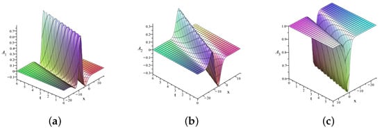
Figure 1. 3D plots of the components of the one-soliton solution of the FLSS. The parameters are $\alpha =1$, $\beta =1$, ${\gamma }_1=2.5$, ${\gamma }_2=2$, $\tau =1$, $\sigma =0.5$, $\gamma =3$, $x\in [-25,15]$ and $t\in [0,6]$. (a) $A_1(x,t)$, (b) $A_2(x,t)$, (c) $A_3(x,t)$.

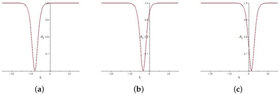
Figure 2. Time evolution of the third component of the one-soliton solution. (a) $t=0$; (b) $t=3$; (c) $t=6$. The parameters are the same as in Figure 1.

These plots clearly demonstrate the localized and stable structure of the obtained one-soliton solution generated by the DT. The wave profile preserves its shape during propagation, indicating elastic behavior and soliton stability. Thus, the visualization of the vector components emphasizes the physical interpretation of the FLSS as an integrable model describing soliton dynamics in ferromagnetic media.

The results obtained for the (1+1)-dimensional systems provide a solid foundation for extending the model to the more general (2+1)-dimensional case. To accomplish this, it is necessary to carry out a detailed analysis of the (2+1)-dimensional FL equation. In the next section, we construct the DT for the (2+1)-dimensional equation and derive the corresponding one- and two-soliton solutions.

3. Exact Soliton Solution of the (2+1)-Dimensional FL Equation

Before applying the Darboux method to the (2+1)-dimensional FL equation, it is useful to highlight the connection with the (1+1)-dimensional case. In the one-dimensional case, the wave evolves only along the coordinate x, whereas the extension to the (2+1)-dimensional case introduces a transverse coordinate y, allowing the system to form more complex localized structures such as dromions, lumps, and vortices. This extension also opens new opportunities for investigating integrable spin systems and the topological properties of solutions.

The study of solitons and their solutions is an active area of research in both physics and mathematics. Among the existing methods for obtaining soliton and other exact solutions of integrable equations, the DT is one of the most powerful tools. Matveev showed that the method proposed by Jean Gaston Darboux for second-order spectral problems and ordinary differential equations can be extended to certain important soliton equations. This method became known as the DT [41,42]. The essence of the DT lies in its ability to generate new solutions from known ones, and it plays a significant role in mechanics, physics, and differential geometry [43].

In this section, the DT method is applied to construct a one-soliton solution of the (2+1)-dimensional FL equation, which was first introduced in [36], and takes the following form:

$$\begin{array}{c}\hfill i{q}_{xt}-i{q}_{xy}+2q_x-q_{x}qr+iq=0,\end{array}$$

(80)

$$\begin{array}{c}\hfill i{r}_{xt}-i{r}_{xy}-2r_x+r_{x}rq+ir=0,\end{array}$$

(81)

where x, y, and t are independent variables, the subscripts denote partial derivatives, with q and r being conjugate fields.

3.1. One-Fold DT of the (2+1)-Dimensional FL Equation

The LR for Equations (80) and (81) takes the following form:

$$\begin{array}{ccc}\hfill {\psi }_x& =& U\psi ,\hfill \end{array}$$

(82)

$$\begin{array}{ccc}\hfill {\psi }_t& =& {\psi }_y+W\psi ,\hfill \end{array}$$

(83)

where $\psi ={({\psi }_1,{\psi }_2)}^T$ (with T denoting transposition), $\lambda$ is the spectral parameter, and the matrix operators U and W are defined as

$$\begin{array}{ccc}\hfill U& =& -i{\lambda }^2{\sigma }_3+\lambda Q,\hfill \\ \hfill W& =& W_0+{\displaystyle \frac{1}{\lambda }}{W}_{-1}-{\displaystyle \frac{i}{4{\lambda }^2}}{\sigma }_3,\hfill \end{array}$$

with

$$Q=\left(\begin{array}{cc}0& q_x\\ r_x& 0\end{array}\right),W_0=i{\sigma }_3-{\displaystyle \frac{iqr}{2}}{\sigma }_3,W_{-1}={\displaystyle \frac{i}{2}}\left(\begin{array}{cc}0& q\\ -r& 0\end{array}\right),{\sigma }_3=\left(\begin{array}{cc}1& 0\\ 0& -1\end{array}\right).$$

To ensure that $L^{\left[1\right]}$ preserves the structure of Equations (80)–(81), the compatibility condition must hold

$${\psi }^{\left[1\right]}=L^{\left[1\right]}\psi =(\lambda N+M+{\lambda }^{-1}K)\psi ,$$

where N, M, and K are matrices of the form

$$N=\left(\begin{array}{cc}{a}_1& b_1\\ c_1& d_1\end{array}\right),M=\left(\begin{array}{cc}{a}_0& b_0\\ c_0& d_0\end{array}\right),K=\left(\begin{array}{cc}{a}_{-1}& b_{-1}\\ c_{-1}& d_{-1}\end{array}\right),$$

where $a_0$, $b_0$, $c_0$, $d_0$, $a_1$, $b_1$, $c_1$, $d_1$, $a_{-1},b_{-1},c_{-1}$ and $d_{-1}$ are functions of x and t.

To ensure that $L^{\left[1\right]}$ preserves the structure of Equations (80)–(81), the following compatibility conditions must be satisfied:

$$\begin{array}{ccc}\hfill L_x^{\left[1\right]}+L^{\left[1\right]}U& =& U^{\left[1\right]}{L}^{\left[1\right]},\hfill \end{array}$$

(84)

$$\begin{array}{ccc}\hfill L_t^{\left[1\right]}+L^{\left[1\right]}W& =& L_y^{\left[1\right]}+W^{\left[1\right]}{L}^{\left[1\right]}.\hfill \end{array}$$

(85)

Equation (84) gives

$$\lambda N_x+M_x+{\lambda }^{-1}{K}_x+\left(\lambda N+M+{\lambda }^{-1}K\right)\left(J{\lambda }^2+Q\lambda \right)=\left(J{\lambda }^2+Q^{\left[1\right]}\lambda \right)\left(\lambda N+M+{\lambda }^{-1}K\right)$$

(86)

By equating the coefficients of Equation (86) at the powers of $\lambda$, we obtain the following system of conditions:

$$\begin{array}{ccc}\hfill M_x+KQ& =& Q^{\left[1\right]}K,\hfill \end{array}$$

(87)

$$\begin{array}{ccc}\hfill N_x+MQ-iK{\sigma }_3& =& Q^{\left[1\right]}M-i{\sigma }_{3}K,\hfill \end{array}$$

(88)

$$\begin{array}{ccc}\hfill NQ-iM{\sigma }_3& =& Q^{\left[1\right]}N-i{\sigma }_{3}M,\hfill \end{array}$$

(89)

$$\begin{array}{ccc}\hfill K_x& =& 0,\hfill \end{array}$$

(90)

$$\begin{array}{ccc}\hfill N{\sigma }_3& =& {\sigma }_{3}N.\hfill \end{array}$$

(91)

From Equation (91), we immediately find

$$b_1=0,c_1=0.$$

Equations (87)–(90) yield differential constraints on the elements of the matrices M and K involving $q_x$, $r_x$, $q_x^{\left[1\right]}$, $r_x^{\left[1\right]}$, and other parameters of the DT.

Equation (85) gives

$$\lambda N_{1t}+M_{1t}+{\lambda }^{-1}{K}_{1t}+\left(\lambda N_1+M_1+{\lambda }^{-1}{K}_1\right)\left(W_0+{\displaystyle \frac{1}{\lambda }}{W}_{-1}-{\displaystyle \frac{i}{4{\lambda }^2}}{\sigma }_3\right)=$$

$$=\lambda N_{1y}+M_{1y}+{\lambda }^{-1}{K}_{1y}+\left(W_0^{\left[1\right]}+{\displaystyle \frac{1}{\lambda }}{W}_{-1}^{\left[1\right]}-{\displaystyle \frac{i}{4{\lambda }^2}}{\sigma }_3\right)\left(\lambda N_1+M_1+{\lambda }^{-1}{K}_1\right).$$

(92)

Similarly, comparing powers of $\lambda$ in Equation (92) yields

$$\begin{array}{ccc}\hfill N_t+N{W}_0& =& N_y+W_0^{\left[1\right]}N,\hfill \end{array}$$

(93)

$$\begin{array}{ccc}\hfill M_t+M{W}_0+N{W}_{-1}& =& M_y+W_{-1}^{\left[1\right]}N+W_0^{\left[1\right]}M,\hfill \end{array}$$

(94)

$$\begin{array}{ccc}\hfill K_t+K{W}_0+M{W}_{-1}-{\displaystyle \frac{i}{4}}N{\sigma }_3& =& K_y+W_{-1}^{\left[1\right]}M+W_0^{\left[1\right]}K-{\displaystyle \frac{i}{4}}{\sigma }_{3}N,\hfill \end{array}$$

(95)

$$\begin{array}{ccc}\hfill K{W}_{-1}-{\displaystyle \frac{i}{4}}M{\sigma }_3& =& W_{-1}^{\left[1\right]}K-{\displaystyle \frac{i}{4}}{\sigma }_{3}M,\hfill \end{array}$$

(96)

$$\begin{array}{ccc}\hfill -{\displaystyle \frac{i}{4}}K{\sigma }_3& =& -{\displaystyle \frac{i}{4}}{\sigma }_{3}K.\hfill \end{array}$$

(97)

From the last condition (97), it follows that

$$b_{-1}=0,c_{-1}=0.$$

From Equation (96), we derive the additional relations

$$\begin{array}{ccc}\hfill b_0+q{a}_{-1}-q^{\left[1\right]}{d}_{-1}& =& 0,\hfill \\ \hfill c_0+r{d}_{-1}-r^{\left[1\right]}{a}_{-1}& =& 0.\hfill \end{array}$$

Now, let us choose $a_{-1}=d_{-1}=a_1=d_1=1$, then the Darboux operator takes the form

$$L^{\left[1\right]}=\lambda I+M+{\lambda }^{-1}I,$$

where I is the identity matrix.

Thus, the one-fold DT for the (2+1)-dimensional FL equation yields the following expressions for the new solutions

$$\begin{array}{ccc}\hfill q^{\left[1\right]}& =& q+b_0,\hfill \end{array}$$

(98)

$$\begin{array}{ccc}\hfill r^{\left[1\right]}& =& r+c_0.\hfill \end{array}$$

(99)

The constructed one-soliton solution of Equations (80) and (81) is further used to obtain explicit analytical formulas and perform spatiotemporal analysis of the excitation described by the $q^{\left[1\right]}$ component.

For more illustrative and constructive representation, and for subsequent application of the DT, it is useful to express the one-fold transformation through eigenfunctions, which will be addressed in the following subsection.

One-Fold DT in Terms of Eigenfunctions

Let the column vector ${({\psi }_1,{\psi }_2)}^T$ be a solution of the Lax pair Equations (82) and (83) for a spectral parameter $\lambda$. Then, the conjugate vector ${(-{\psi }_2^{*},{\psi }_1^{*})}^T$ is also a solution of the same Lax pair but corresponding to the conjugate spectral parameter ${\lambda }^{*}$. This property allows us to construct the DT matrix M using eigenfunctions in the following form:

$$M=H{\Lambda }^{-1}{H}^{-1},$$

(100)

where H is the fundamental matrix composed of the eigenfunctions

$$H=\left(\begin{array}{cc}{\psi }_1({\lambda }_1,t,x,y)& -{\psi }_2^{*}({\lambda }_1,t,x,y)\\ {\psi }_2({\lambda }_1,t,x,y)& {\psi }_1^{*}({\lambda }_1,t,x,y)\end{array}\right),H^{-1}={\displaystyle \frac{1}{\Delta }}\left(\begin{array}{cc}{\psi }_1^{*}& {\psi }_2^{*}\\ -{\psi }_2& {\psi }_1\end{array}\right),$$

(101)

with $\Lambda =\mathrm{diag}({\lambda }_1,{\lambda }_2)$, ${\lambda }_2={\lambda }_1^{*}={\lambda }^{*}$, and the normalization factor $\Delta =|{\psi }_1{|}^2+{|{\psi }_2|}^2$.

Substituting Equation (101) into (100), we obtain the explicit form of the matrix M,

$$M={\displaystyle \frac{1}{\Delta }}\left(\begin{array}{cc}{\lambda }^{-1}|{\psi }_1{|}^2+{\left({\lambda }^{*}\right)}^{-1}{|{\psi }_2|}^2& ({\lambda }^{-1}-{\left({\lambda }^{*}\right)}^{-1}){\psi }_1{\psi }_2^{*}\\ ({\lambda }^{-1}-{\left({\lambda }^{*}\right)}^{-1}){\psi }_1^{*}{\psi }_2& {\lambda }^{-1}|{\psi }_2{|}^2+{\left({\lambda }^{*}\right)}^{-1}{|{\psi }_1|}^2\end{array}\right).$$

(102)

From Equation (102), the expressions for the elements $b_0$ and $c_0$ of the Darboux matrix are obtained directly,

$$\begin{array}{ccc}\hfill b_0& =& {\displaystyle \frac{({\lambda }^{-1}-{\left({\lambda }^{*}\right)}^{-1}){\psi }_1{\psi }_2^{*}}{\Delta }},\hfill \\ \hfill c_0& =& {\displaystyle \frac{({\lambda }^{-1}-{\left({\lambda }^{*}\right)}^{-1}){\psi }_1^{*}{\psi }_2}{\Delta }}.\hfill \end{array}$$

Thus, the transformed fields $q^{\left[1\right]}$ and $r^{\left[1\right]}$ resulting from the one-fold DT are expressed in terms of the eigenfunction components as follows:

$$\begin{array}{ccc}\hfill q^{\left[1\right]}& =& q+{\displaystyle \frac{({\lambda }^{-1}-{\lambda }^{*-1}){\psi }_1{\psi }_2^{*}}{\Delta }},\hfill \end{array}$$

(103)

$$\begin{array}{ccc}\hfill r^{\left[1\right]}& =& r+{\displaystyle \frac{({\lambda }^{-1}-{\lambda }^{*-1}){\psi }_1^{*}{\psi }_2}{\Delta }}.\hfill \end{array}$$

(104)

These expressions serve as a key foundation for constructing explicit soliton solutions of the (2+1)-dimensional FL equation, which will be presented in the following subsections.

3.2. Two-Fold DT of the (2+1)-Dimensional FL Equation

Building upon the previously established one-fold DT, we now proceed to its second iteration to obtain more complex solutions, in particular two-soliton configurations. This iterative framework leverages the algebraic structure of the DT, where each successive step is constructed based on the outcome of the preceding one.

Let ${\Phi }^{\left[2\right]}$ denote the result of applying a two-fold DT to the initial field $\Phi$,

$${\Phi }^{\left[2\right]}=L^{\left[2\right]}{\Phi }^{\left[1\right]},$$

(105)

where $L^{\left[2\right]}$ is the second-order Darboux matrix, defined by

$$L^{\left[2\right]}=\lambda I+M^{\left[2\right]}+{\lambda }^{-1}I.$$

(106)

Here, $M^{\left[2\right]}$ is a matrix depending on the eigenfunctions introduced at the second step.

Combining the successive DT, we obtain

$${\Phi }^{\left[2\right]}=L^{\left[2\right]}{L}^{\left[1\right]}\Phi =\left[(\lambda I+M^{\left[2\right]}+{\lambda }^{-1}I)(\lambda I+M^{\left[1\right]}+{\lambda }^{-1}I)\right]\Phi .$$

(107)

Since this product yields a quadratic polynomial in $\lambda$, we define the following coefficients for convenience:

$$l_2^0=I,l_2^1=M^{\left[1\right]}+M^{\left[2\right]},l_2^2=M^{\left[2\right]}{M}^{\left[1\right]},$$

(108)

allowing us to rewrite $L^{\left[2\right]}$ in compact polynomial form

$$L^{\left[2\right]}=({\lambda }^2+{\lambda }^{-2}+2)l_2^0+(\lambda +{\lambda }^{-1})l_2^1+l_2^2.$$

(109)

Substituting $L^{\left[2\right]}$ into the Lax compatibility conditions

$$\begin{array}{ccc}\hfill L_x^{\left[2\right]}+L^{\left[2\right]}U& =& U^{\left[2\right]}{L}^{\left[2\right]},\hfill \end{array}$$

(110)

$$\begin{array}{ccc}\hfill L_t^{\left[2\right]}+L^{\left[2\right]}W& =& L_y^{\left[2\right]}+W^{\left[2\right]}{L}^{\left[2\right]},\hfill \end{array}$$

(111)

and comparing terms with like powers of $\lambda$, one can derive evolution equations for the transformed potentials $q^{\left[2\right]}$ and $r^{\left[2\right]}$.

The result of this procedure yields explicit expressions for the fields

$$\begin{array}{ccc}\hfill q^{\left[2\right]}& =& q+b_0+b_0^{\left[1\right]},\hfill \end{array}$$

(112)

$$\begin{array}{ccc}\hfill r^{\left[2\right]}& =& r+c_0+c_0^{\left[1\right]}.\hfill \end{array}$$

(113)

Thus, the two-fold DT provides an effective mechanism for iteratively generating higher-order solutions of the original nonlinear system, enabling the construction of multi-soliton configurations and their interactions.

3.3. N-Fold DT of the (2+1)-Dimensional FL Equation

The N-fold DT is obtained by successive application of the one-fold DT. The corresponding Darboux matrix has the product form

$$L^{\left[n\right]}\left(\lambda \right)=\prod _{k=1}^n(\lambda I+M^{\left[k\right]}+{\lambda }^{-1}I),{\psi }^{\left[n\right]}=L^{\left[n\right]}\left(\lambda \right)\psi ,$$

(114)

where each $M^{\left[k\right]}$ is constructed from the eigenfunctions introduced at the k-th step. Expanding this product gives the Laurent form

$$L^{\left[n\right]}\left(\lambda \right)=\sum _{j=-n}^n{\lambda }^j{L}_j^{\left[n\right]}.$$

(115)

The new potentials are obtained iteratively as

$$q^{\left[n\right]}=q+\sum _{k=0}^{n-1}{b}_0^{\left[k\right]},r^{\left[n\right]}=r+\sum _{k=0}^{n-1}{c}_0^{\left[k\right]},$$

(116)

which generalizes the one- and two-fold results and allows the construction of multi-soliton solutions.

3.4. One-Soliton Solution of the (2+1)-Dimensional FL Equation

In this section, we derive the exact one-soliton solution of Equations (80) and (81) using the one-fold DT. We take the trivial seed solution $q=0$ with vanishing boundary conditions

$$q(x,y,t)\to 0,q_x(x,y,t)\to 0,r(x,y,t)\to 0,\mathrm{as}|x|,|y|\to \infty .$$

The resulting system takes the form

$$\begin{array}{ccc}\hfill {\psi }_{1x}& =& -i{\lambda }^2{\psi }_1,\hfill \end{array}$$

(117)

$$\begin{array}{ccc}\hfill {\psi }_{2x}& =& i{\lambda }^2{\psi }_2,\hfill \end{array}$$

(118)

$$\begin{array}{ccc}\hfill {\psi }_{1t}& =& {\psi }_{1y}+i\left(1-{\displaystyle \frac{1}{4{\lambda }^2}}\right){\psi }_1,\hfill \end{array}$$

(119)

$$\begin{array}{ccc}\hfill {\psi }_{2t}& =& {\psi }_{2y}-i\left(1-{\displaystyle \frac{1}{4{\lambda }^2}}\right){\psi }_2.\hfill \end{array}$$

(120)

These equations admit exponential solutions of the form

$$\begin{array}{ccc}\hfill {\psi }_1& =& k_1{e}^{-i{\lambda }^{2}x+i{\mu }_{1}y+i\left({\mu }_1+1-{\displaystyle \frac{1}{4{\lambda }^2}}\right)t+i{\eta }_1}=k_1{e}^{{\theta }_1},\hfill \end{array}$$

(121)

$$\begin{array}{ccc}\hfill {\psi }_2& =& k_2{e}^{i{\lambda }^{2}x+i{\mu }_{2}y+i\left({\mu }_2-1+{\displaystyle \frac{1}{4{\lambda }^2}}\right)t+i{\eta }_2}=k_2{e}^{{\theta }_2},\hfill \end{array}$$

(122)

where ${\mu }_1,{\mu }_2,k_1,k_2,{\eta }_1,{\eta }_2$ are arbitrary complex parameters. We write

$${\mu }_n={\omega }_n+i{\nu }_n,{\eta }_n={\kappa }_n+i{\chi }_n,n=1,2,$$

and

$$k_1=|k_1|e^{i{\vartheta }_1},k_2=|k_2|e^{i{\vartheta }_2},{\displaystyle \frac{|k_1|}{|k_2|}}=e^{2\vartheta }.$$

Here, $\alpha ,\beta ,{\omega }_n,{\nu }_n,{\kappa }_n,{\chi }_n\in \mathbb{R}$ denote the real and imaginary parts of the respective complex parameters.

The one-soliton solution of Equations (103) and (104) can be written in the following form:

$$q^{\left[1\right]}={\displaystyle \frac{\left(\frac{1}{\lambda }-\frac{1}{{\lambda }^{*}}\right)e^{i({\vartheta }_1-{\vartheta }_2+{\theta }_1-{\theta }_1^{*})}}{2\cosh (2\vartheta +{\theta }_1+{\theta }_1^{*})}}.$$

(123)

Thus,

$${\theta }_1=-i{\lambda }^{2}x+i{\mu }_{1}y+i\left({\mu }_1+1-{\displaystyle \frac{1}{4{\lambda }^2}}\right)t+i{\eta }_1.$$

Assuming ${\mu }_2={\mu }_1$ and ${\eta }_2=-{\eta }_1$, we obtain ${\theta }_2=-{\theta }_1$.

Figure 3 illustrates the propagation of the one-soliton solution described by Equation (123) for $t=0.5$, with parameters $M_1=1+i$ and ${\delta }_1=1$: (a) $\lambda =1+i$, (b) $\lambda =1+2i$, (c) $\lambda =1-2i$.

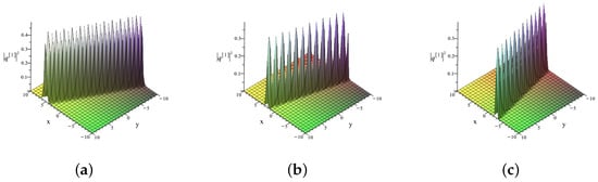
Figure 3. 3D plots of $q^{\left[1\right]}$ at different parameter values.(a) For $\lambda =1+i$, (b) For $\lambda =1+2i$, (c) For $\lambda =1-2i$.

Figure 3a–c shows three-dimensional profiles of the soliton at time $t=0.5$ for various values of the spectral parameter $\lambda$. In each case, a clearly localized solitary wave is observed, aligned along the diagonal in the $(x,y)$-plane.

Figure 3a corresponds to $\lambda =1+i$. In this case, a well-localized soliton with relatively high amplitude and smooth spatial shape is observed. The wave is concentrated along the diagonal direction of the $(x,y)$-plane, indicating stable propagation without noticeable oscillations.

For $\lambda =1+2i$, shown in Figure 3b, the soliton profile becomes slightly elongated, and its amplitude decreases. Weak spatial oscillations appear, reflecting enhanced dispersive effects and the influence of the increased imaginary part of the spectral parameter. The resulting waveform demonstrates a modulated structure caused by the interplay between dispersion and localization.

In Figure 3c, corresponding to $\lambda =1-2i$, the soliton maintains its localized nature but exhibits a mirrored spatial profile relative to Figure 3b. The direction of propagation is reversed, showing that the sign of the imaginary part of $\lambda$ determines the orientation and phase behavior of the soliton wave.

Overall, the variation in the spectral parameter $\lambda$ mainly affects the amplitude, direction, and modulation of the soliton, while its localized and stable structure remains preserved.

Denoting ${\theta }_1=\rho +iϵ$ and $\lambda =\alpha +i\beta$, the real and imaginary parts are given by

$$\begin{array}{ccc}\hfill \rho & =& 2\alpha \beta x-{\nu }_{1}y-\left({\nu }_1+{\displaystyle \frac{\alpha \beta }{2{({\alpha }^2+{\beta }^2)}^2}}\right)t-{\chi }_1,\hfill \end{array}$$

(124)

$$\begin{array}{ccc}\hfill ϵ& =& -({\alpha }^2-{\beta }^2)x+{\omega }_{1}y+\left({\omega }_1+1-{\displaystyle \frac{{\alpha }^2-{\beta }^2}{4{({\alpha }^2+{\beta }^2)}^2}}\right)t+{\kappa }_1.\hfill \end{array}$$

(125)

The corresponding eigenfunctions become

$$\begin{array}{ccc}\hfill {\psi }_1& =& k_1{e}^{\rho +iϵ},\hfill \end{array}$$

(126)

$$\begin{array}{ccc}\hfill {\psi }_2& =& k_2{e}^{-\rho -iϵ}.\hfill \end{array}$$

(127)

Substituting these into the Darboux Equations (103) and (104) yields the exact one-soliton solution

$$q^{\left[1\right]}=-{\displaystyle \frac{i\beta e^{i(2ϵ+{\vartheta }_1-{\vartheta }_2)}}{({\alpha }^2+{\beta }^2)\cosh 2(\vartheta +\rho )}}.$$

(128)

To illustrate the spatiotemporal dynamics of the one-soliton solution of the (2+1)-dimensional FL equation, Figure 4 and Figure 5 present the plots of the field component $|q^{\left[1\right]}{|}^2$. The simulations were performed for the spectral parameter $\lambda =1+i$ and the parameter values: ${\omega }_1=2$, ${\nu }_1=1$, ${\chi }_1=1$, ${\kappa }_1=1$.

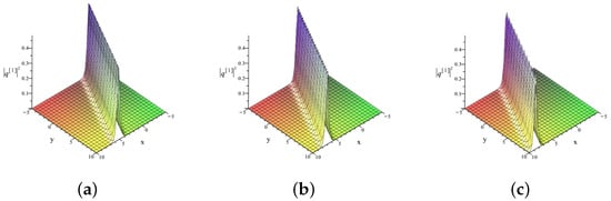
Figure 4. 3D plots of the field component ${|q(x,y,t)}^{\left[1\right]}{|}^2$ of the one-soliton solution of the (2+1)-dimensional FL equation at the spectral parameter $\lambda =1+i$. (a) $t=0$; (b) $t=3$; (c) $t=6$. The parameters are $x\in [-5,10]$ and $y\in [-5,10]$.

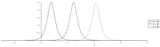
Figure 5. Time evolution of the one-soliton solution $|q^{\left[1\right]}{|}^2$ of the (2+1)-dimensional FL equation. The solid, dashed, and dash-dotted lines correspond to the time moments $t=0$, $t=3$, and $t=6$ for the parameters $\alpha =1$, $\beta =1$, ${\omega }_1=2$, ${\nu }_1=1$, ${\chi }_1=1$, ${\kappa }_1=1$.

Figure 4 shows the temporal evolution of $|q^{\left[1\right]}{|}^2$ at different time moments $t=0,3,6$, while Figure 5 presents the 3D surface plot of ${|q(x,y,t)}^{\left[1\right]}{|}^2$. The solid, dashed, and dash-dotted lines represent these times, respectively. The results clearly demonstrate that the soliton maintains a localized and stable profile during propagation, confirming the integrability and elastic nature of the nonlinear dynamics governed by the (2+1)-dimensional FL equation.

In summary, the obtained one-soliton solution shows that the wave preserves its shape and localization during propagation, confirming the stability and integrable nature of the system. In the next section, this approach is extended to the two-soliton case to study the interaction between the waves.

3.5. Two-Soliton Solutions of the (2+1)-Dimensional FL Equation

We now proceed to construct the two-soliton solution of the (2+1)-dimensional FL equation. To this end, consider the transformation

$${\Phi }^{\left[2\right]}=L^{\left[2\right]}{\Phi }^{\left[1\right]},$$

(129)

where the Darboux matrix is defined as

$$L^{\left[2\right]}=\lambda I+M^{\left[2\right]}+{\lambda }^{-1}I=(\lambda +{\lambda }^{-1})I+M^{\left[2\right]}.$$

(130)

The fields ${\Phi }^{\left[j\right]}$ satisfy the following Lax pair systems:

$$\begin{array}{ccc}\hfill {\Phi }_x^{\left[2\right]}& =& U^{\left[2\right]}{\Phi }^{\left[2\right]},\hfill \end{array}$$

(131)

$$\begin{array}{ccc}\hfill {\Phi }_t^{\left[2\right]}& =& {\Phi }_y^{\left[2\right]}+W^{\left[2\right]}{\Phi }^{\left[2\right]},\hfill \end{array}$$

(132)

$$\begin{array}{ccc}\hfill {\Phi }_x^{\left[1\right]}& =& U^{\left[1\right]}{\Phi }^{\left[1\right]},\hfill \end{array}$$

(133)

$$\begin{array}{ccc}\hfill {\Phi }_t^{\left[1\right]}& =& {\Phi }_y^{\left[1\right]}+W^{\left[1\right]}{\Phi }^{\left[1\right]}.\hfill \end{array}$$

(134)

The Darboux matrix $L^{\left[2\right]}$ satisfies the compatibility (intertwining) relations

$$\begin{array}{ccc}\hfill L_x^{\left[2\right]}+L^{\left[2\right]}{U}^{\left[1\right]}& =& U^{\left[2\right]}{L}^{\left[2\right]},\hfill \end{array}$$

(135)

$$\begin{array}{ccc}\hfill L_t^{\left[2\right]}+L^{\left[2\right]}{W}^{\left[1\right]}& =& L_y^{\left[2\right]}+W^{\left[2\right]}{L}^{\left[2\right]}.\hfill \end{array}$$

(136)

In terms of eigenfunctions, the matrix $M^{\left[2\right]}$ takes the form

$$M^{\left[2\right]}={\displaystyle \frac{1}{{\Delta }^{\left[1\right]}}}\left(\begin{array}{cc}{\lambda }_3^{-1}|{\Phi }_1^{\left[1\right]}{|}^2+{\lambda }_4^{-1}{|{\Phi }_2^{\left[1\right]}|}^2& ({\lambda }_3^{-1}-{\lambda }_4^{-1}){\Phi }_1^{\left[1\right]}{\Phi }_2^{\left[1\right]*}\\ ({\lambda }_3^{-1}-{\lambda }_4^{-1}){\Phi }_1^{\left[1\right]*}{\Phi }_2^{\left[1\right]}& {\lambda }_4^{-1}|{\Phi }_2^{\left[1\right]}{|}^2+{\lambda }_3^{-1}{|{\Phi }_1^{\left[1\right]}|}^2\end{array}\right),$$

(137)

with ${\lambda }_4={\lambda }_3^{*}$.

To obtain the components of ${\Phi }^{\left[1\right]}$, we apply the one-fold DT

$${\Phi }^{\left[1\right]}=L^{\left[1\right]}{\Phi }^{\left[0\right]},$$

(138)

where

$$\begin{array}{ccc}\hfill {\Phi }^{\left[0\right]}& =& \left(\begin{array}{cc}{\Psi }_1\left({\lambda }_1\right)& -{\Psi }_2^{*}\left({\lambda }_1\right)\\ {\Psi }_2\left({\lambda }_1\right)& {\Psi }_1^{*}\left({\lambda }_1\right)\end{array}\right),\hfill \end{array}$$

(139)

$$\begin{array}{ccc}\hfill L^{\left[1\right]}& =& \left(\begin{array}{cc}{\lambda }_3+{\lambda }_3^{-1}& b_0\\ c_0& {\lambda }_3+{\lambda }_3^{-1}\end{array}\right).\hfill \end{array}$$

(140)

Substituting Equations (139) and (140) into Equation (138) yields

$${\Psi }^{\left[1\right]}=\left(\begin{array}{cc}{\Psi }_1^{\left[1\right]}& -{\Psi }_2^{\left[1\right]*}\\ {\Psi }_2^{\left[1\right]}& {\Psi }_1^{\left[1\right]*}\end{array}\right)=\left(\begin{array}{cc}({\lambda }_3+{\lambda }_3^{-1}){\Psi }_1+b_0{\Psi }_2& -({\lambda }_3+{\lambda }_3^{-1}){\Psi }_2^{*}+b_0{\Psi }_1^{*}\\ ({\lambda }_3+{\lambda }_3^{-1}){\Psi }_2-b_0^{*}{\Psi }_1& ({\lambda }_3+{\lambda }_3^{-1}){\Psi }_1^{*}+b_0^{*}{\Psi }_2^{*}\end{array}\right),$$

(141)

where

$$\begin{array}{ccc}\hfill {\Psi }_1^{\left[1\right]}& =& ({\lambda }_3+{\lambda }_3^{-1})|k_3|e^{i{\vartheta }_3+{\rho }_2+i{ϵ}_2}+b_0|k_4|e^{i{\vartheta }_4-{\rho }_2-i{ϵ}_2},\hfill \\ \hfill {\Psi }_2^{\left[1\right]}& =& ({\lambda }_3+{\lambda }_3^{-1})|k_4|e^{i{\vartheta }_4-{\rho }_2-i{ϵ}_2}-b_0^{*}|k_3|e^{i{\vartheta }_3+{\rho }_2+i{ϵ}_2},\hfill \\ \hfill {\Delta }^{\left[1\right]}& =& 2|k_3||k_4|\cosh \left(2(\zeta +{\rho }_2)\right)\left[{({\lambda }_3+{\lambda }_3^{-1})}^2+{|b_0|}^2\right].\hfill \end{array}$$

and ${\lambda }_3={\alpha }_3+i{\beta }_3$.

The explicit two-soliton solution is obtained via the two-fold DT from the same trivial seed $q=0$.

$$\begin{array}{c}\hfill q^{\left[2\right]}=b_0+{\displaystyle \frac{({\lambda }_3-{\lambda }_3^{*-1})|k_3||k_4|}{{\Delta }^{\left[1\right]}}}\left[{({\lambda }_3+{\lambda }_3^{-1})}^2{e}^{i({\vartheta }_3-{\vartheta }_4+2{ϵ}_2)}-2({\lambda }_3+{\lambda }_3^{-1})b_0\sinh \left(2(\zeta +{\rho }_2)\right)-b_0^2{e}^{-i({\vartheta }_3-{\vartheta }_4+2{ϵ}_2)}\right],\end{array}$$

(142)

where

$$\begin{array}{ccc}\hfill {\rho }_2& =& 2{\alpha }_3{\beta }_{3}x-{\nu }_{3}y-\left({\nu }_3+{\displaystyle \frac{{\alpha }_3{\beta }_3}{2{({\alpha }_3^2+{\beta }_3^2)}^2}}\right)t-{\chi }_3,\hfill \\ \hfill {ϵ}_2& =& -({\alpha }_3^2-{\beta }_3^2)x+{\omega }_{3}y+\left({\omega }_3+1-{\displaystyle \frac{({\alpha }_3^2-{\beta }_3^2)}{4{({\alpha }_3^2+{\beta }_3^2)}^2}}\right)t+{\kappa }_3,\hfill \end{array}$$

and

$$k_3=|k_3|e^{i{\vartheta }_3},k_4=|k_4|e^{i{\vartheta }_4},{\displaystyle \frac{|k_3|}{|k_4|}}=e^{2\zeta },{\displaystyle \frac{|k_4|}{|k_3|}}=e^{-2\zeta },{\vartheta }_3,{\vartheta }_4,\zeta \in \mathbb{R}.$$

The graphical representation of the two-soliton solution $q^{\left[2\right]}$ of the (2+1)-dimensional FL equation is presented in Figure 6 and Figure 7.

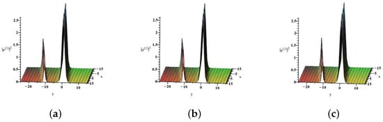
Figure 6. 3D plots of the two-soliton solution $|q^{\left[2\right]}{|}^2$ of the (2+1)-dimensional FL equation at different time moments: (a) $t=0$, (b) $t=3$, and (c) $t=6$.

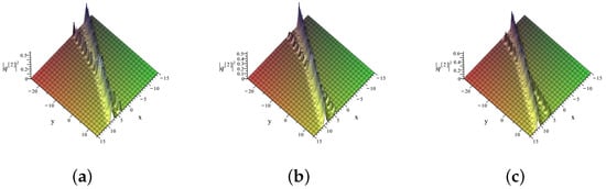
Figure 7. 3D plots of the two-soliton solution $|q^{\left[2\right]}{|}^2$ of the (2+1)-dimensional FL equation illustrating the elastic collision of two intersecting linear solitons at different time moments: (a) $t=0$, (b) $t=3$ and (c) $t=6$.

Figure 6 illustrates the two-dimensional structure of $q^{\left[2\right]}$, showing two localized amplitude peaks of $|q^{\left[2\right]}|$ in the $(x,y)$ plane at different time moments $t=0,3$, and 6. At $t=0$, the solitons are well-separated and exhibit sharp, high peaks. As time progresses, the positions and shapes of the peaks evolve, reflecting the solitons’ interaction and propagation. Despite these changes, each soliton preserves its characteristic form, which is typical for solitonic solutions of nonlinear equations.

Figure 7 provides a complementary 3D visualization, highlighting the elastic collision of the two solitons. The snapshots at $t=0$, 3, and 6 demonstrate that, although the solitons interact and undergo small phase shifts, they retain their amplitudes and shapes after the collision. This confirms the elastic nature of the interaction and the integrability of the (2+1)-dimensional FL model. The parameters used are ${\alpha }_4=2$, ${\beta }_4=2$, ${\omega }_3=2$, with the spatial domain $x\in [-15,15]$ and $y\in [-25,25]$. Figure 6 shows the graphical representation of the two-dimensional two-soliton solution $q^{\left[2\right]}$ given by Equation (142).

Overall, the two-soliton solution $q^{\left[2\right]}$ captures both the mathematical structure and the physical behavior of nonlinear wave propagation in optical fibers, plasma, or ferromagnetic media, providing insight into stable, interacting soliton dynamics.

4. Conclusions

In this study, we explored an integrable extension of the nonlinear Schrödinger equation, known as the FL equation, which plays a crucial role in modern nonlinear wave theory and accounts for higher-order dispersion as well as nonlinear effects. Owing to its complete integrability, the FL equation admits exact analytical solutions and serves as a foundation for constructing related models, including spin systems and equations with self-consistent sources.

We first derived a novel (1+1)-dimensional FL equation with self-consistent sources, enabling the study of soliton interactions with external perturbations within an integrable framework. For this model, we constructed the associated Lax pair and implemented the DT, confirming the system’s integrability.

Moreover, we presented for the first time two types of analytical solutions for a spin system that is gauge equivalent to the FL equation: a traveling wave and a one-soliton solution. These were obtained using the DT and further analyzed through visualizations of the spin vector components, demonstrating their localized structure and physical relevance in ferromagnetic media.

For the (2+1)-dimensional FL equation, we constructed explicit one- and two-soliton solutions using the DT. Analytical and graphical analyses elucidated the influence of key parameters on soliton dynamics, particularly highlighting their roles in shaping the soliton’s width, amplitude, propagation velocity, and phase structure. In particular, the parameters $\alpha$ and $\beta$ characterize the soliton’s spatial extent and propagation speed, which are of direct physical significance.

In summary, the findings of this work contribute to a deeper understanding of integrable systems and enrich the methodology for analyzing nonlinear evolution equations. These results have potential applications in the theory of optical solitons, spin wave dynamics, quantum fluids, and broader areas of mathematical physics and soliton theory.

References

- Wazwaz, A.M. Partial Differential Equations and Solitary Waves Theory; Springer: Berlin/Heidelberg, Germany, 2009. [Google Scholar]
- Dodd, R.K.; Eilbeck, J.C.; Gibbon, J.D.; Morris, H.C. Solitons and Nonlinear Wave Equations; Academic Press: London, UK, 1982. [Google Scholar]
- Ablowitz, M.J.; Clarkson, P.A. Solitons, Nonlinear Evolution Equations and Inverse Scattering; Cambridge University Press: Cambridge, UK, 1991. [Google Scholar]
- Liu, J.G.; Zhu, W.H. Multiple rogue wave, breather wave and interaction solutions of a generalized (3+1)-dimensional variable-coefficient nonlinear wave equation. Nonlinear Dyn. 2021, 103, 1841–1850. [Google Scholar] [CrossRef]
- Burdik, C.; Shaikhova, G.; Rakhimzhanov, B. Soliton solutions and travelling wave solutions for the two-dimensional generalized nonlinear Schrödinger equations. Eur. Phys. J. Plus 2021, 136, 1095. [Google Scholar] [CrossRef]
- Yao, S.W.; Behera, S.; Inc, M.; Rezazadeh, H.; Virdi, J.P.S.; Mahmoud, W.; Arqu, O.A.; Osman, M.S. Analytical solutions of conformable Drinfel’d-Sokolov-Wilson and Boiti-Leon-Pempinelli equations via sine-cosine method. Results Phys. 2022, 42, 105990. [Google Scholar] [CrossRef]
- Yesmakhanova, K.; Bekova, G.; Shaikhova, G.; Myrzakulov, R. Soliton solutions of the (2+1)-dimensional complex modified Korteweg-de Vries and Maxwell–Bloch equations. J. Phys. Conf. Ser. 2016, 738, 012018. [Google Scholar] [CrossRef]
- Chen, H.; Zheng, S. Darboux transformation for nonlinear Schrödinger type hierarchies. Phys. D 2023, 454, 133863. [Google Scholar] [CrossRef]
- Yesmakhanova, K.; Bekova, G.; Myrzakulov, R.; Shaikhova, G. Lax representation and soliton solutions for the (2+1)-dimensional two-component complex modified Korteweg-de Vries equations. J. Phys. Conf. Ser. 2017, 804, 012004. [Google Scholar]
- Wazwaz, A.M. The Tanh and the Sine-Cosine Methods for the Complex Modified KdV and the Generalized KdV Equations. Comput. Math. Appl. 2005, 49, 1101–1112. [Google Scholar] [CrossRef]
- Shaikhova, G.N.; Kutum, B.B.; Myrzakulov, R. Periodic traveling wave, bright and dark soliton solutions of the (2+1)-dimensional complex modified Korteweg-de Vries system of equations by using three different methods. AIMS Math. 2022, 7, 18948–18970. [Google Scholar] [CrossRef]
- Fokas, A.S. On a class of physically important integrable equations. Phys. D 1995, 87, 145–150. [Google Scholar] [CrossRef]
- Lenells, J.; Fokas, A.S. On a novel integrable generalization of the nonlinear Schrödinger equation. Nonlinearity 2009, 22, 11–27. [Google Scholar] [CrossRef]
- Lenells, J. Exactly solvable model for nonlinear pulse propagation in optical fibers. Stud. Appl. Math. 2009, 123, 215–232. [Google Scholar] [CrossRef]
- Lenells, J. Dressing for a novel integrable generalization of the nonlinear Schrödinger equation. J. Nonlinear Sci. 2010, 20, 709–722. [Google Scholar] [CrossRef]
- Geng, X.-G.; Guo, F.-Y.; Zhai, Y.-Y. Two integrable generalizations of WKI and FL equations: Positive and negative flows, and conservation laws. Chin. Phys. B 2020, 29, 050201. [Google Scholar] [CrossRef]
- Lenells, J. The derivative nonlinear Schrödinger equation on the half-line. Phys. D 2009, 240, 512–530. [Google Scholar] [CrossRef][Green Version]
- Matsuno, Y. Multisoliton solutions of the Fokas–Lenells equation and their properties. J. Phys. Soc. Jpn. 2012, 81, 034002. [Google Scholar][Green Version]
- Ling, A.; Ling, L. The Riemann-Hilbert approach for the integrable fractional Fokas-Lenells equation. Appl. Math. Lett. 2019, 87, 57–63. [Google Scholar][Green Version]
- Huang, J.; Xu, S.; Kuppuswamy, P. Rogue waves of the Fokas-Lenells equation. J. Phys. Soc. Jpn. 2012, 81, 124007. [Google Scholar][Green Version]
- Matsuno, Y. A direct method of solution for the Fokas-Lenells derivative nonlinear Schrödinger equation: I. Bright soliton solutions. J. Phys. A Math. Theor. 2012, 45, 235201. [Google Scholar] [CrossRef]
- Matsuno, Y. A direct method of solution for the Fokas-Lenells derivative nonlinear Schrödinger equation: II. Dark soliton solutions. J. Phys. A Math. Theor. 2012, 45, 475201. [Google Scholar] [CrossRef]
- Ling, L.; Feng, B.-F.; Zhu, Z. General soliton solutions to a coupled Fokas-Lenells equation. Nonlinear Anal. Real World Appl. 2018, 40, 185–214. [Google Scholar] [CrossRef]
- Li, J.; Xia, T. N-soliton solutions for the nonlocal Fokas-Lenells equation via RHP. Appl. Math. Lett. 2021, 113, 106850. [Google Scholar] [CrossRef]
- Melnikov, V.K. Integration method of the KdV equation with a self-consistent source. Commun. Math. Phys. 1990, 126, 201–215. [Google Scholar] [CrossRef]
- Chvartatskyi, O. On integrable equations with self-consistent sources. J. Math. Phys. 2015, 56, 103506. [Google Scholar]
- Doliwa, A.; Lin, R. Discrete KP equation with self-consistent sources. Phys. Lett. A 2014, 378, 1925–1931. [Google Scholar] [CrossRef]
- Mel’nikov, V. Integration of the nonlinear Schrödinger equation with a source. Inverse Probl. 1992, 8, 133–147. [Google Scholar] [CrossRef]
- Reyimberganov, A.A.; Rakhimov, I.D. The soliton solutions for the nonlinear Schrödinger equa-tion with self-consistent source. Bull. Irkutsk State Univ. Ser. Math. 2021, 36, 84–94. [Google Scholar]
- Wei, J.; Geng, X.; Wang, X. An integrable generalization of the Fokas-Lenells equation: Darboux transformation, reduction and explicit soliton solutions. Chin. Phys. B 2024, 33, 070202. [Google Scholar] [CrossRef]
- Manikandan, K.; Serikbayev, N.; Vijayasree, S.P.; Aravinthan, D. Controlling Matter-Wave Smooth Positons in Bose–Einstein Condensates. Symmetry 2023, 15, 1585. [Google Scholar] [CrossRef]
- Zahran, E.H.M.; Ahmad, H.; Rahaman, M.; Ibrahim, R.A. Soliton solutions in (2+1)-dimensional integrable spin systems: An investigation of the Myrzakulov-Lakshmanan equation-II. Opt. Quantum Electron. 2024, 56, 895. [Google Scholar] [CrossRef]
- Lakshmanan, M. Continuum spin system as an exactly solvable dynamical system. Phys. Lett. A 1977, 61, 53–54. [Google Scholar] [CrossRef]
- Saleem, U.; Hasan, M. Quasideterminant solutions of the generalized Heisenberg magnet model. J. Phys. A Math. Theor. 2010, 43, 045204. [Google Scholar] [CrossRef]
- Huang, N.-N.; Xu, B. Darboux Transformation Method for Finding Soliton Solutions of the Landau-Lifshitz Equation of a Classical Heisenberg Spin Chain. Commun. Theor. Phys. 1989, 12, 121–126. [Google Scholar] [CrossRef]
- Zhassybayeva, M.; Bekova, G.; Yesmakhanova, K.; Myrzakulov, R. Integrable motions of curves of the induced Fokas-Lenells equation. Optik 2023, 286, 170979. [Google Scholar] [CrossRef]
- Serikbayev, N.; Saparbekova, A. Symmetry and conservation laws of the (2+1)-dimensional nonlinear Schrödinger-type equation. Int. J. Geom. Methods Mod. Phys. 2023, 20, 2350172. [Google Scholar] [CrossRef]
- Zhao, Q.; Song, H.; Li, X. Higher-order rogue wave solutions of the (2+1)-dimensional Fokas-Lenells equation. Wave Motion 2022, 115, 103065. [Google Scholar] [CrossRef]
- Guan, Y.; Li, X.; Zhao, Q. Interaction wave solutions of the (2+1)-dimensional Fokas-Lenells equation. Phys. Scr. 2021, 100, 045219. [Google Scholar] [CrossRef]
- Zhao, Q.; Zhang, X.; Li, X. Classification of solutions for the (2+1)-dimensional Fokas-Lenells equations based on bilinear method and Wronskian technique. Nonlinear Dyn. 2025, 113, 2569–2597. [Google Scholar] [CrossRef]
- Matveev, V.B.; Salle, M.A. Darboux Transformations and Solitons; Springer: Berlin/Heidelberg, Germany, 1991. [Google Scholar]
- Rogers, C.; Schief, W.K. Bäcklund and Darboux Transformations: Geometry and Modern Applications in Soliton Theory; Cambridge University Press: Cambridge, UK, 2002. [Google Scholar]
- Novikov, S.P.; Manakov, S.V.; Pitaevskii, L.P.; Zakharov, V.E. Theory of Solitons: The Inverse Scattering Method; Springer: Berlin/Heidelberg, Germany, 1984. [Google Scholar]
Disclaimer/Publisher’s Note: The statements, opinions and data contained in all publications are solely those of the individual author(s) and contributor(s) and not of MDPI and/or the editor(s). MDPI and/or the editor(s) disclaim responsibility for any injury to people or property resulting from any ideas, methods, instructions or products referred to in the content. |
© 2025 by the authors. Licensee MDPI, Basel, Switzerland. This article is an open access article distributed under the terms and conditions of the Creative Commons Attribution (CC BY) license (https://creativecommons.org/licenses/by/4.0/).