Article

A Collaborative Optimization Strategy for Photovoltaic Array Layout Based on the Lemur Optimization Algorithm

1
School of Automation, Guangdong University of Technology, Guangzhou 510006, China
2
School of Electrical Engineering, Southeast University, Nanjing 210096, China
3
School of Electrical Engineering, China University of Mining and Technology, Xuzhou 221116, China
*
Author to whom correspondence should be addressed.
Symmetry 2025, 17(11), 1870; https://doi.org/10.3390/sym17111870
Submission received: 3 September 2025 / Revised: 27 September 2025 / Accepted: 1 October 2025 / Published: 5 November 2025
(This article belongs to the Special Issue Symmetry in Digitalisation of Distribution Power System)

Abstract

The performance of large-scale photovoltaic (PV) power plants is strongly influenced by array layout parameters including module tilt angle, azimuth angle, and row spacing. These geometric variables jointly determine solar irradiance geometry, shading losses, and land-use efficiency, affecting annual energy yield and levelized cost of electricity. To achieve multi-objective comprehensive optimization of array layout parameters for a PV power generation system, a collaborative optimization strategy for PV array layout based on the lemur optimization (LO) algorithm is proposed in this paper. The method couples the Perez anisotropic irradiance model with a dynamic shading irradiance geometric model to simulate the effective insolation, incorporating land availability, shading thresholds, and maintenance access requirements. In addition, the LO algorithm is employed to solve resulting nonlinear and constrained problems, enabling an efficient global search across large parameter spaces. The case studies in Lianyungang, Dalian, and Fuzhou City show that the proposed scheme based on the LO algorithm improves annual energy yield compared with the existing optimization schemes, providing new theoretical methods and engineering application paths for the optimal layout of PV arrays.

1. Introduction

Driven by the global energy transition and carbon neutrality goals, photovoltaic (PV) power generation has become one of the core directions for renewable energy deployment due to its clean, scalable, and cost-effective advantages. Consequently, the construction of large-scale PV power plants is rapidly expanding worldwide. Under limited land and engineering constraints, the performance of PV systems depends not only on the technical and material properties of PV modules but also on their layout parameters, including tilt angle, azimuth angle, and row spacing. These geometric parameters jointly determine the incidence geometry, dynamic shading conditions, and land-use efficiency, thereby directly affecting annual energy yield and cost of electricity [1,2,3]. The layout issue of photovoltaic arrays is essentially a systematic subject that seeks the best balance between symmetry and defect breaking. Ideally, a completely symmetrical array—components neatly arranged at equal intervals and angles without any obstructions—corresponds to maximized spatial symmetry. This symmetry is the perfect configuration for achieving maximum energy output under uniform illumination without external interference. However, in the actual operating environment, the solar altitude angle and azimuth angle change nonlinearly over time. The terrain, surrounding obstructions, and shadows generated by the array itself introduce strong non-uniform disturbances, leading to the breaking of symmetry [4,5,6]. Therefore, during the design phase of photovoltaic power plants, comprehensively considering solar irradiance characteristics, geographical location, meteorological conditions, and site constraints to optimize module layout parameters has become a critical step in enhancing the economic efficiency and energy performance of PV power systems.
In the optimization layout of photovoltaic arrays, the optimization of tilt angle, azimuth angle, and row spacing is essentially the process of seeking dynamic symmetry and balance in the spatiotemporal dimension between the system’s energy capture capability and external driving sources as well as its own constraints. It is a process of counterbalancing and compensating for the native asymmetry brought about by solar movement and terrain constraints through the introduction of meticulous intervention. Thus, it is a systematic scientific practice to achieve a dynamic balance of system energy capture at a higher dimension [7,8]. The existing literature presents its theoretical and application progress. The foundation of PV performance evaluation and optimization lies in accurately estimating the irradiance incident on module surfaces, which relies on precise solar position algorithms and irradiance transposition models [9,10]. Existing solar position methods include Astronomical Algorithms, the Solar Position Algorithm, and various refined models proposed by U.S. National Renewable Energy Laboratory [11,12]. For tilted-plane irradiance estimation, the Perez anisotropic irradiance model is widely adopted due to its high accuracy and adaptability under diverse meteorological conditions [13,14,15,16]. However, in practical operation, the mutual shading between photovoltaic modules causes uneven illumination within the array, which not only leads to output power degradation but also may result in reliability risks such as the “hot spot effect” [17,18,19]. Shading simulation methods include geometric projection, ray tracing, and image-based algorithms. The geometric methods are computationally efficient and well-suited for large-scale dynamic shading analysis, whereas ray tracing offers higher accuracy in complex terrains at the expense of significantly increased computational costs [20,21,22,23]. Despite progress in irradiance transposition and shading prediction, a critical challenge remains in achieving high accuracy while maintaining computational efficiency, particularly when integrating dynamic shading effects into a year-round, hourly simulation framework [24].
The spatial configuration of PV arrays critically influences solar energy capture, shading losses, and land-use efficiency, in which the core geometric parameters include module tilt angle, azimuth angle, and row spacing [25,26]. Early studies primarily focused on optimizing a single parameter. For fixed-tilt systems, the annual optimal tilt and azimuth angles were derived from irradiance data and empirical formulas to maximize solar utilization [27,28,29]. For spacing optimization, geometric shading models or seasonal solar altitude analysis were used to determine the minimum shading-free distance [30]. Subsequent studies have begun to consider the two parameters as coupled optimization variables (e.g., tilt-azimuth or tilt-spacing), using two-parameter models to capture their nonlinear interactions and determine their joint optimal values under different seasons, latitudes, and climate conditions [31,32]. However, dual- parameter optimization remains insufficient to capture the full coupling effects among all three core geometric parameters. Moreover, most current formulated optimization problems focus on maximizing irradiance or power generation, without systematically incorporating actual engineering constraints such as land area restrictions, shading loss thresholds, operation and maintenance channels, and ventilation conditions [33].
In terms of optimization methods, meta-heuristic optimization algorithms such as particle swarm optimization (PSO), genetic algorithm (GA), and ant colony optimization (ACO) have made rapid progress in recent years, which are widely used in the multi-parameter collaborative optimization of photovoltaic arrays [34,35,36]. These algorithms exhibit strong global search and convergence capabilities in solving nonlinear and constrained optimization problems. In addition, the improved gray wolf optimization (IGWO) algorithm effectively balances global exploration and local development capabilities by introducing nonlinear convergence factors and hybrid search strategies, thereby enhancing the accuracy and speed of maximum power point tracking under local shadows. The hybrid algorithm of particle swarm optimization and gray wolf optimization (PSO-GWO) integrates the fast convergence of PSO and global optimization advantages of GWO and is used for parameter identification of PV array models, significantly improving model accuracy and convergence stability. In addition, new algorithms such as the sandcat swarm optimization (SCSO) algorithm have been proposed, aiming to solve layout optimization problems under multi-peak and high-dimensional constraints, demonstrating good adaptability [37,38,39]. However, many long-term hourly simulations neglect the coupled influence of irradiance and temperature dynamics on PV performance, potentially leading to deviations in real-world operation [40].
To solve the above problem, this study proposes a collaborative optimization strategy for PV array layout based on the lemur optimization (LO) algorithm, with tilt angle, azimuth angle, and row spacing as the core decision variables. The proposed framework incorporates land area limitations, dynamic inter-row shading, and meteorological conditions as constraints, and employs the LO algorithm to maximize annual energy yield. The main contributions of this paper are listed as follows:
  • A novel PV array design framework that combines the Perez anisotropic irradiance model with a dynamic shading irradiance geometric model to jointly model the irradiance and shading is proposed, thereby enabling the accurate estimation of long-term effective irradiance.
  • The proposed framework introduces tilt angle, azimuth angle, and row spacing as coupled decision variables, incorporating land area, shading loss, and maintenance constraints into the optimization problem to enhance engineering practicality and application feasibility.
  • The proposed framework employs the LO algorithm to effectively solve the three-variable PV array layout problem, demonstrating superior convergence efficiency and solution quality compared with conventional optimization algorithms such as PSO and GA, thereby validating the effectiveness and robustness of the proposed design methodology.
The remainder of this paper is organized as follows. Section 2 presents the three- variable collaborative optimization framework for PV array design, including the mathematical models for solar geometry, solar radiation, hourly shading analysis, and the optimization objective of maximizing annual irradiance under engineering constraints. Section 3 describes the LO algorithm for PV array layout, covering its principles, encoding, and implementation for optimizing the triple variables tilt angle, azimuth angle, and row spacing. Section 4 presents a case study in Lianyungang, Dalian, and Fuzhou City. Section 5 concludes the paper.

2. Collaborative Optimization Framework for PV Array Layout Design

In general, the framework evaluates the solar irradiance received and effectively utilized by PV arrays’ layout with varying tilt angle β , azimuth angle γ , and row spacing D . Therefore, the mathematical models of the three-variable collaborative optimization framework for PV array design are presented. The solar geometry model that determines the incident angles of direct and diffuse radiation on module surfaces is discussed (Section 2.1). Then, the Perez anisotropic irradiance model is employed to estimate tilted-surface irradiance under real-sky conditions, capturing anisotropic diffuse components (Section 2.2). Third, a dynamic geometric shading model quantifies inter-row shading losses throughout the year at hourly resolutions (Section 2.3). Finally, the annual irradiance per unit area is calculated and incorporated into the proposed objective function, along with engineering constraints related to land area, shading, and structural requirements (Section 2.4). These models together form the theoretical basis for the optimization framework.

2.1. Mathematical Model of Solar Angles

The sun is the primary source of solar energy, with its radiation reaching earth at an average intensity of 1367 W/m2, known as the solar constant, as defined by the World Radiation Center (WRC) [41].
The magnitude of solar irradiation depends on the angle of the sun and the angle of the components, as shown in Figure 1. Among them, the solar zenith angle and the solar azimuth angle describe the position of the sun in the sky and determine the availability of direct irradiation. The tilt angle and azimuth angle of the component define the orientation of the component and affect the projection mode of sunlight on the component plane. The relationship between them will be described in detail below.
The tilt angle δ , which reflects the seasonal tilt between the sun and earth’s equator, ranges from −23.45° to +23.45° due to the axial tilt and is commonly estimated using Cooper’s equation [42].
  δ = 23.45 s i n 360 284 + n 365  
where n denotes the specific day of the calendar year.
The incident angle θ is defined as the angle between the incoming solar rays and the surface normal. For a horizontal surface, it is calculated as:
cos θ = s i n φ s i n δ + c o s φ c o s δ c o s ω
where φ is the site’s geographic latitude and ω is the solar hour angle. For south-facing tilted surfaces in the northern hemisphere, Equation (2) can be simplified to:
  cos θ = c o s δ c o s φ β c o s ω + s i n δ s i n φ β
where β represents the tilt angle between the horizontal plane and the surface receiving solar radiation.
The solar hour angle ω measures sun’s angular shift from solar noon 0°, changing by 15° per hour. Under AST, it is positive in the afternoon and negative in morning [43].
  ω = 15 × A S T 12
The solar azimuth angle γ s is the angle between sun’s horizontal projection and true south, calculated from the hour angle, declination, and zenith angle θ z e n [43,44]:
  γ s = s i g n w c o s 1 c o s θ z e n s i n φ s i n δ s i n θ z e n c o s φ
The solar zenith angle θ z e n is the angle between sun and vertical axis, and it can be calculated as follows [44]:
cos θ z e n = cos δ cos φ cos ω + sin φ sin δ
The solar altitude angle, indicating the sun’s height above horizon, is key to PV tilt optimization and is calculated from the declination and hour angles via [45]:
  cos θ z e n = sin α s
  α s = a r c s i n c o s θ z e n
In the northern hemisphere, sunrise and sunset occur when the solar zenith angle θ z e n = 0 . The sunset hour angle ω s u n s e t is then calculated as [46]:
  ω s u n s e t = min c o s 1 tan φ tan δ c o s 1 tan φ β tan δ
Then, the following equation is applied to determine the time of sunset t s u n s e t :
t s u n s e t = c o s 1 tan φ · tan δ 2 15 °
For a tilted surface, sunrise and sunset times can differ from those on a horizontal plane, often reducing solar exposure. For a south-facing surface, sunset time t s u n s e t . s o u t h is calculated as:
  t s u n s e t . s o u t h   = min ω s u n s e t × c o s 1 tan φ β · tan δ 2 15 °

2.2. Solar Radiation Modeling Based on the Perez Anisotropic Irradiance Model

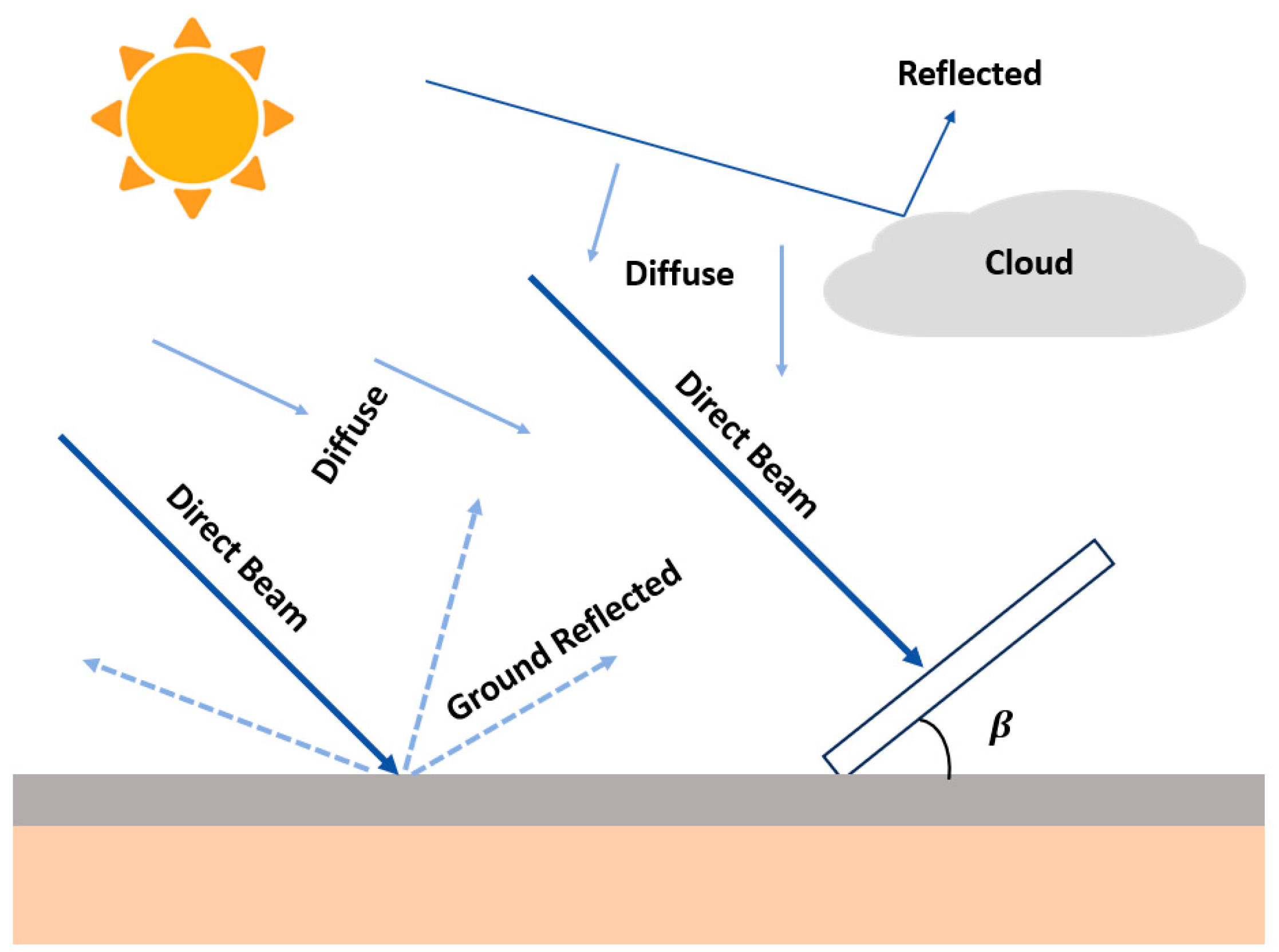
The solar radiation model uses mathematical formulas to estimate total irradiance on tilted surfaces. Accurate assessment of the solar resource for PV modules requires integrated modeling of solar position dynamics across different orientations, tilt angles, and site-specific geographic conditions. Key factors include geographic coordinates, solar time calculations, temporal parameters, and solar geometry. Total radiation on an inclined plane combines direct beam radiation H B , diffuse radiation H D , and ground-reflected radiation H R , as shown in Figure 2.
Therefore, the overall irradiance can be calculated as:
  H T = H B + H D +   H R
Direct irradiance on a tilted PV surface is proportional to the beam irradiance on a horizontal plane and can be calculated using Equation (13).
  H B , T = cos ( θ ) cos ( θ z e n ) H b
where H B , T is the hourly beam irradiance on the tilted PV surface and H b is the hourly beam irradiance on the horizontal plane.
The anisotropic sky model improves diffuse irradiance estimates from the isotropic model. The Perez model further refines this by incorporating empirical parameters for greater accuracy. The diffuse irradiance on an inclined surface using the Perez model can be calculated as:
  H D , T = H d 1 F 1 1 + c o s β 2 + F 1 a b + F 2 s i n β
where F 1 and F 2 are dimensionless circumsolar and horizontal brightness coefficients, respectively. These parameters describe sky conditions based on solar zenith angle θ z e n , atmospheric clearness, and brightness index , as defined in Equations (15) and (16).
  F 1 = max 0 ,   f 11 + f 12 + π θ z e n 180 ° f 13
  F 2 = f 21 + f 22 + π θ z e n 180 ° f 23
Then, the brightness index is defined by:
  = m H d G S C
where m is the air mass, representing the atmospheric path length that sunlight travels. G S C is the solar constant. Its theoretical calculation is given by:
  m = 1 cos ( θ z e n )
The clearness index ξ is defined by the ratio between the diffuse irradiance H d and the direct beam irradiance H n on a surface perpendicular to the sun’s rays:
ξ = H d + H n H d + 5.535 × 10 e 6 θ z e n 3 1 + 5.535 × 10 e 6 θ z e n 3 f 23
In the equation, the brightness coefficients f 11 , f 12 , f 23 are empirical constants.
In the Perez model, the coefficients a and b adjust for the angular effect of the solar cone on both inclined and horizontal surfaces. This study treats the sun as a point source when considering circumsolar irradiance. The related equations are given by:
  a = m a x 0 , cos ( θ z e n )
  b = m a x cos 85 ° , cos ( θ z e n )
The reflected component primarily involves the surface reflectance and tilt angle β , and it can be expressed as:
  H R = H b + H d ρ 1 + c o s ( β ) 2
where ρ is the ground reflectance varying with surface type.
In summary, the hourly solar irradiance on a tilted PV surface is given by:
  H T = cos ( θ ) cos ( θ z e n ) H b + H d 1 F 1 1 + c o s β 2 + H d F 1 a b + H d F 2 s i n β + H b + H d ρ 1 + c o s ( β ) 2
From (23), the hourly solar irradiance on a tilted PV surface consists of five components: direct beam irradiance, anisotropic diffuse irradiance, circumsolar diffuse irradiance, isotropic horizontal diffuse irradiance, and ground-reflected irradiance.

2.3. Dynamic Shading Irradiance Geometric Model

For a ground-mounted PV array, the shading losses primarily result from mutual shading between parallel rows. Each PV string is uniformly mounted with the same tilt angle β , azimuth angle γ and row spacing D , allowing the shading model to be simplified as the projection between two parallel planes, dependent on solar position.
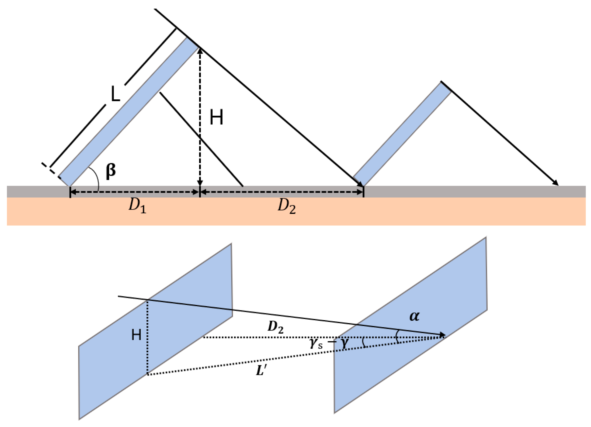
As illustrated in Figure 3, at a specific hour, the minimum row spacing required to avoid shading is given by Equations (24)–(27):
  D t s = D 1 + D 2
  D 1 = L × c o s ( β )
  D 2 = L × c o s ( γ s γ ) × L
  L = H t a n α s
where H is the vertical height of the PV array, D 1 is the projected length through the PV module, D 2 is the reserved spacing between modules in the actual layout, and γ s is the array’s azimuth angle.
The proportion of the shaded area relative to the support structure is given by:
p s h a d = 1 D D t s 0   , D D t s , D < D t s
where D is the actual row spacing. In the string configuration, the shading loss factor depends on the number of PV module rows affected by shading. Let m denote the number of side-by-side rows on a single rack. The shading loss factor is calculated as:
  F s h a d = 1 p s h a d 1 / m × 1 / m
where the square bracket · denotes the ceiling function (rounding up). To obtain the final power irradiance, the loss factor is applied as a coefficient, and can be shown as:
  H s h a d , = H T , i × 1 × F s h a d

2.4. Objective Function and Constraints

2.4.1. Formulation of Objective Function

To enable the rigorous evaluation and optimization of the PV array’s annual energy potential, a high-fidelity mathematical objective function is formulated. This function is designed to precisely quantify the complex, nonlinear relationship between the three core design variables, tilt angle β , azimuth angle γ , and row spacing D , and the system’s net effective annual irradiance. The construction of this model begins with the analytical principles of instantaneous energy capture and proceeds through a hierarchical temporal integration to establish an annual performance metric capable of guiding a global optimization algorithm.
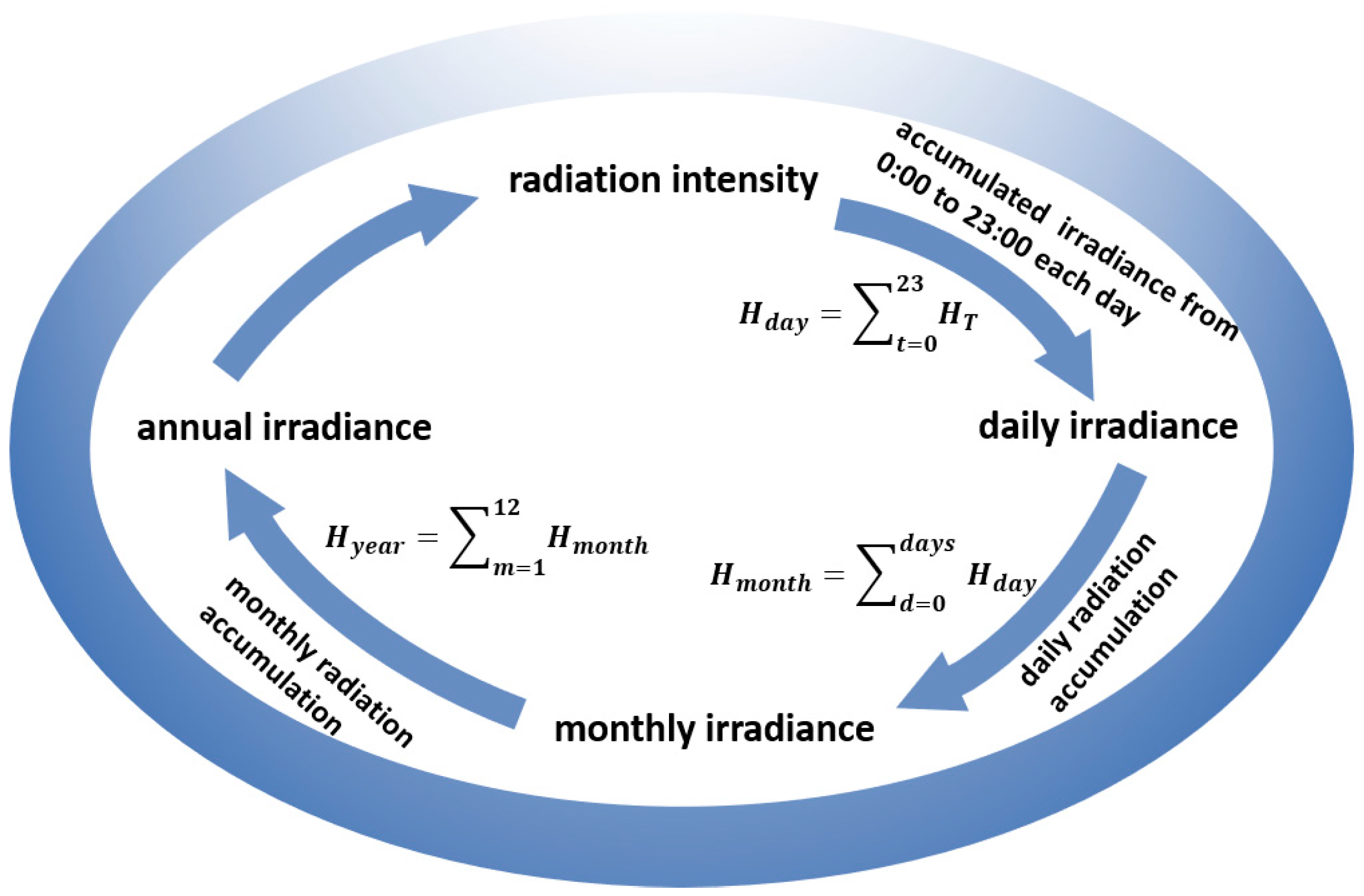
The physical rationale of the model is that the effective irradiance on a photovoltaic surface is proportional to c o s θ , the cosine of the solar incidence angle; hence, maximizing c o s θ serves as a practical proxy for maximizing the energy yield. For an array with an arbitrary spatial orientation, c o s θ is a function of the array parameters β , γ and the instantaneous solar position δ , ω . However, as the PV array in this study is of a fixed-tilt design, its parameters β , γ , D are constant throughout its operational lifetime. The optimization objective thus evolves from an instantaneous goal to the search for a single, fixed set of parameters β , γ , D which maximizes the cumulative net irradiance over an entire year. The model adopts a bottom-up cumulative computational framework, as illustrated in Figure 4.
First, the instantaneous net effective power irradiance H n e t n , t , β , γ , D is defined for hour t on day n of the year. This value represents the actual irradiance received after accounting for dynamic inter-row shading. From (23)–(30), the instantaneous net effective power irradiance can be derived from the product of the total irradiance on the tilted surface H T and the dynamic shading loss factor F s h a d :
H n e t n , t , β , γ , D =   H T n , t , β , γ , D × F s h a d n , t , β , γ , D
Second, by integrating the instantaneous values over all daylight hours from sunrise to sunset, the daily cumulative net effective irradiance E d a y n , t , β , γ , D for day n can be defined as:
  E d a y n , t , β , γ , D =   t = t s u n r i s e ( n ) t s u n s e t ( n ) H T n , t , β , γ , D · t
where t is the time step (1 h in this study), and the t s u n r i s e and t s u n r i s e times are determined by Equations (9) and (10).
Subsequently, the monthly cumulative net effective irradiance for month m , E m o n t h m , t , β , γ , D is calculated by summing daily values for all days within that month.
  E m o n t h n , t , β , γ , D =   n M o n t h ( m )   E d a y n , t , β , γ , D
Finally, the annual optimization objective function f β , γ , D is defined as the sum of the monthly cumulative net effective irradiances over a full year. By substituting the preceding equations hierarchically, the objective function in its complete, multi-level nested form is as follows:
  f β , γ , D = m = 1 12   n M o n t h m   t = t s u n r i s e n t s u n s e t n H T n , t , β , γ , D × F s h a d n , t , β , γ , D  
Therefore, the optimization problem for the proposed three-variable collaborative optimization framework for PV array design is formulated as maximizing the above objective function. This formulation comprehensively integrates solar geometry, the Perez anisotropic irradiance model, and dynamic inter-row shading effects, resulting in a highly coupled nonlinear optimization problem.

2.4.2. Structural Constraints of PV Array Deployment

To ensure physical feasibility and engineering practicality, appropriate constraints must be imposed on the design variables. The specific constraints are defined as follows:
  β m i n β β m a x
  γ m i n γ γ m a x
  D m i n D D m a x
where β m i n and β m a x define the feasible range for tilt angle β , and γ m i n , γ m a x , D m i n , and D m a x similarly bound the azimuth angle γ and array spacing D .
T a , m i n <   T a = T c G t 800 N O C T 20 <   T a , m a x
where T a is the module’s actual operating temperature, while NOCT refers to its rated value under standard tests. Acceptable limits T a , m i n and T a , m a x are defined by material and manufacturing standards.
The modern photovoltaic plant must fit within limited land, so the array layout area cannot exceed the allowed boundary. This limits capacity and affects return on investment:
  A t o t a l = N r o w s × D + L · c o s β × W r o w   A m a x
where A t o t a l is the PV field area, and A m a x is the maximum land area available. N r o w s is the number of rows, W r o w is the width of each row, and L is the module length along the tilt, respectively. This nonlinear constraint connects design variables D and β with layout and economic factors.
To ensure the overall energy performance and asset value of power plant, a clear upper limit is typically imposed on the annual irradiance loss rate caused by shading:
  S l o s s = E u n s h a d e d β , γ f β , γ , D E u n s h a d e d β , γ S m a x
where S l o s s is the annual irradiance loss rate from shading. The function f β , γ , D is the net annual energy yield to be optimized. E u n s h a d e d β , γ is the ideal yield without shading D (i.e., no shading at all). S m a x limits the maximum allowable loss rate, usually 2–3%. This constraint balances land-use and energy output, avoiding excessive losses while maintaining compact layouts.
In addition, to meet the operation and maintenance requirements of PV systems, the design of photovoltaic arrays also needs to take into account the height constraint. Specifically, local zoning and land-use regulations at the project site often impose explicit limits on the maximum height of structures.
  H s t r u c t = L · s i n β + H m o u n t H m a x  
where H s t r u c t is the structure’s highest point from the ground. H m o u n t is the clearance between the lowest point and the ground, while L · s i n β is the module’s vertical height. H m a x is the legal height limit. This constraint sets a clearer legal limit on tilt angle β than the empirical β m a x in Equation (35).
In summary, by constructing multi-dimensional and cross-disciplinary constraint systems, the study transforms an abstract mathematical optimization model into a highly realistic engineering design problem. This ensures that the final optimal solution set β , γ , D achieves globally optimal energy output while fully complying with all practical constraints.

3. The Optimization for PV Array Layout Based on the LO Algorithm

To optimize PV array layout configuration and maximize annual energy yield, an effective optimization framework is needed. This involves formulating a fitness function that captures the impact of geometric variables, tilt angle β , azimuth angle γ , and row spacing D , allowing the evaluation of energy output for each candidate design. The LO algorithm, a metaheuristic method, is employed for its efficiency in exploring complex, high-dimensional, nonlinear solution spaces.

3.1. Fundamental Principles of the Lemurs Optimization Algorithm

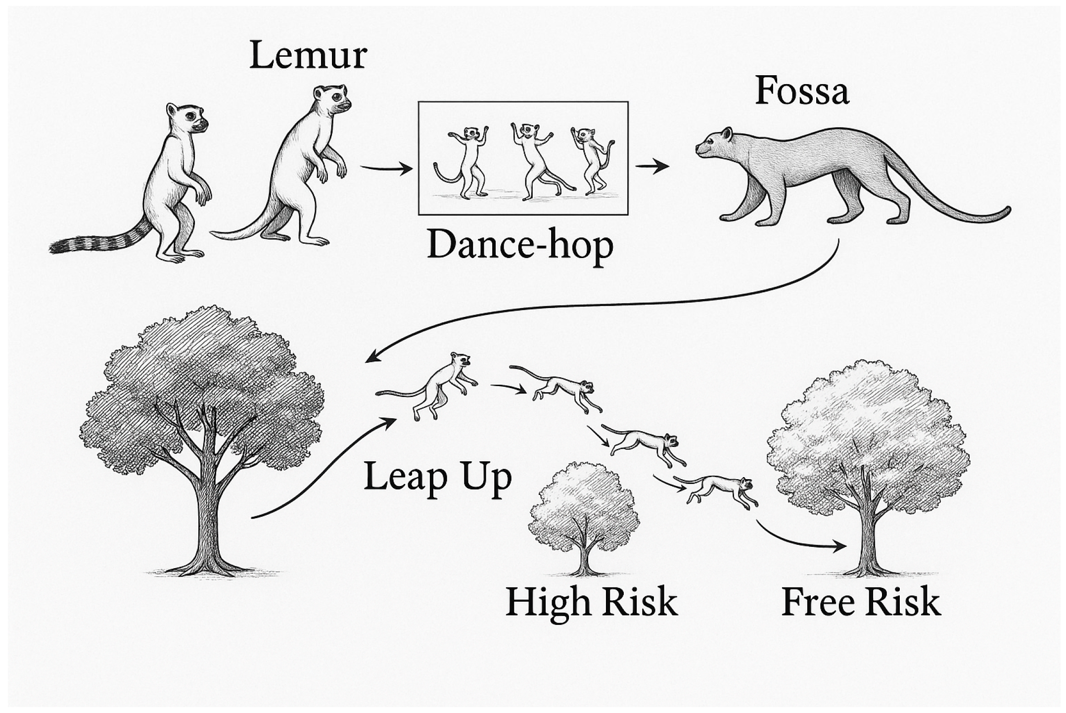
The LO algorithm is a swarm intelligence optimization method based on nature inspiration, with its core being the balance between global exploration and local development. As shown in Figure 5, the algorithm mechanism mainly stems from two behaviors: “Leap-up”, which is used to achieve long-distance exploratory jumps to avoid becoming stuck in local optima; and “Dance-hub” which is used for a concentrated search near potential excellent solutions to fine-tune them [47]. Such a complementary mechanism enables the LO algorithm to exhibit strong robustness when dealing with nonlinear and multimodal optimization problems. In the optimization of photovoltaic module layout, the LO algorithm can flexibly adjust inclination angle, azimuth angle, and row spacing simultaneously, and take into account the constraints of occlusion and site utilization. To maintain a clear structure, this section only introduces the basic principle of the LO algorithm. The theoretical formula of the LO algorithm and its specific combination with photovoltaic layout optimization (including coding methods, constraints, and fitness evaluation) will be elaborated in detail in Section 3.2.
During the optimization, the LO algorithm represents the population as a matrix with each individual corresponding to a feasible solution. The candidate solutions are formed for the current generation. The initial population is defined by the following matrix:
  P = p 11 p 12 p 21 p 22 p 1 r p 21 p t 1 p t 1 p t r
where P represents the population matrix, r denotes the number of design variables, and t is the number of candidate solutions. Thus, the size of population matrix is t × r .
Any random variable i in the solution j is computed as follows:
p i , j = r a n d ( ) × u b i l b i + l b i j 1,2 , , n i 1,2 , , d
where l b j , u b j denotes the bounds of variable i , a random number is produced using the r a n d ( ) function.
During population evolution, lemurs with lower fitness adjust their decision parameters more frequently than fitter ones, promoting solution diversity and driving overall improvement. In each iteration, the local best (i.e., bnl) and the global best (i.e., gbl) lemurs are dynamically identified based on fitness. When updating, the i-th decision variable of solution j is adjusted either toward the global best or influenced by the local best in its neighborhood, and can be defined as:
p i , j = p i , j + a b s p i , j p b n l , j × r a n d 0.5 × 2 , r a n d < F R R   p i , j + a b s p i , j p g b l , j × r a n d 0.5 × , r a n d > F R R
According to the formula, the free risk rate ( F R R ) serves as a crucial regulatory parameter within the LO algorithm. The corresponding calculation formula is as follows:
  F R R = F R R H i g h _ R i s k _ R a t e × C u r r I t e r H i g h _ R i s k _ R a t e L o w _ R i s k _ R a t e M a x I t e r
The constants H i g h _ R i s k _ R a t e and L o w _ R i s k _ R a t e set the allowable F R R range, enabling dynamic adjustment to balance exploration and exploitation during optimization. The C u r r I t e r and M a x I t e r denote the current and maximum iteration counts, respectively.

3.2. The Application of the LO Algorithm in PV Array Layout Optimization

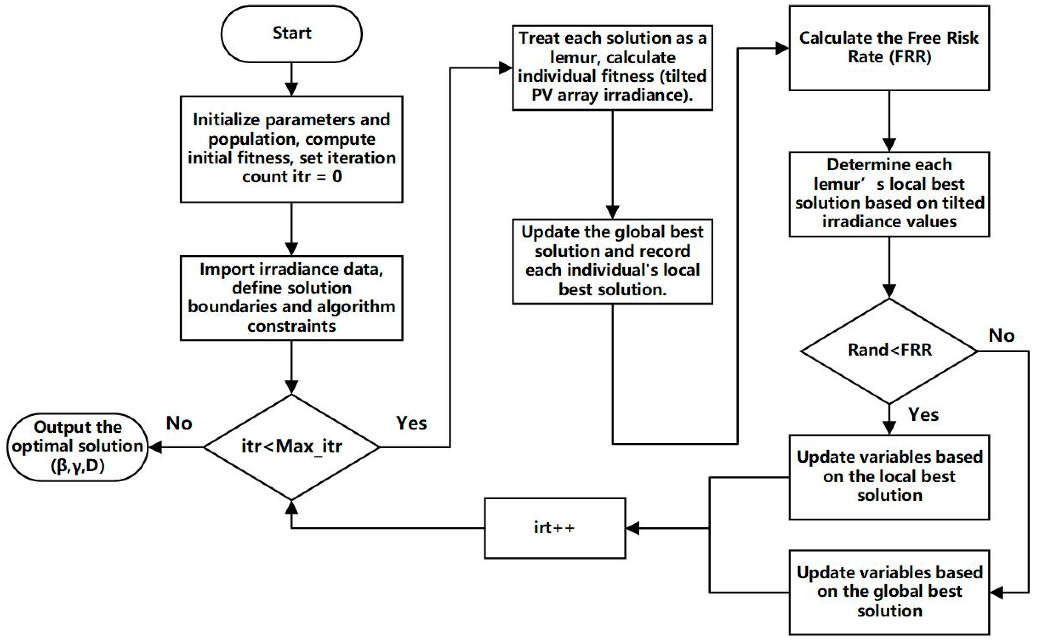
To solve the multivariable, nonlinear, and strongly coupled optimization problem formulated in Section 2.4, aimed at maximizing the annual total effective irradiance, this study introduces the LO algorithm as the core optimization tool. The algorithm follows a rigorous computational procedure designed to efficiently explore the complex solution space defined by the tilt angle β , azimuth angle γ , and row spacing D , ultimately converging to the global optimum. The entire optimization process is illustrated in the framework shown in Figure 6.
Step 1: Problem Definition and Parameter Initialization:
  • Define the objective as maximizing annual effective irradiance H s h a d , accounting for dynamic shading;
  • Encode each solution as a vector of three variables—tilt angle β , azimuth angle γ , and row spacing D ;
  • Generate the initial population matrix P with t candidate solutions, initializing each variable within its physical bounds, as defined in Equation (42).
Step 2: Fitness Evaluation:
  • Evaluate each individual using the objective function f β , γ , D defined in Section 2.4;
  • Irradiance is calculated hourly by first computing the total irradiance on the tilted surface H T , then applying the shading loss factor F s h a d to obtain effective irradiance H s h a d . Summing hourly values yields daily, monthly, and annual totals, which serve as the fitness score;
  • Identify the global best individual ( g b l ) with the highest fitness and record local bests ( b n l ) within each neighborhood.
Step 3: Iterative Update and Optimization:
  • Update individual positions: iteratively update the position of each individual in the population β , γ , D according to Equation (43);
  • Search behavior is controlled by the free risk rate ( F R R ). If a random number exceeds the F R R , the individual moves toward the global best ( g b l ) with a large exploratory step (leaping upward). If below the F R R , the individual refines its position near the local best (dancing center);
  • F R R is adaptively adjusted at each iteration using Equation (45), decreasing linearly from the H i g h _ R i s k _ R a t e to the L o w _ R i s k _ R a t e as the iteration count increases. This mechanism enhances early stage exploration and late-stage convergence.
Step 4: Termination and Output:
  • Repeat Steps 2 and 3 until the termination condition is met, typically when the maximum number of iterations is reached;
  • Once terminated, the algorithm outputs the global best solution P g b l = β g b l , γ g b l , D g b l , representing the optimal layout configuration that maximizes annual energy yield.

4. Case Study and Analysis

4.1. Case Setup and Data Description

To comprehensively validate the effectiveness and generalizability of the proposed PV array spatial optimization strategy based on the LO algorithm, a comparative case study was conducted across three representative locations in China with distinct climatic characteristics:
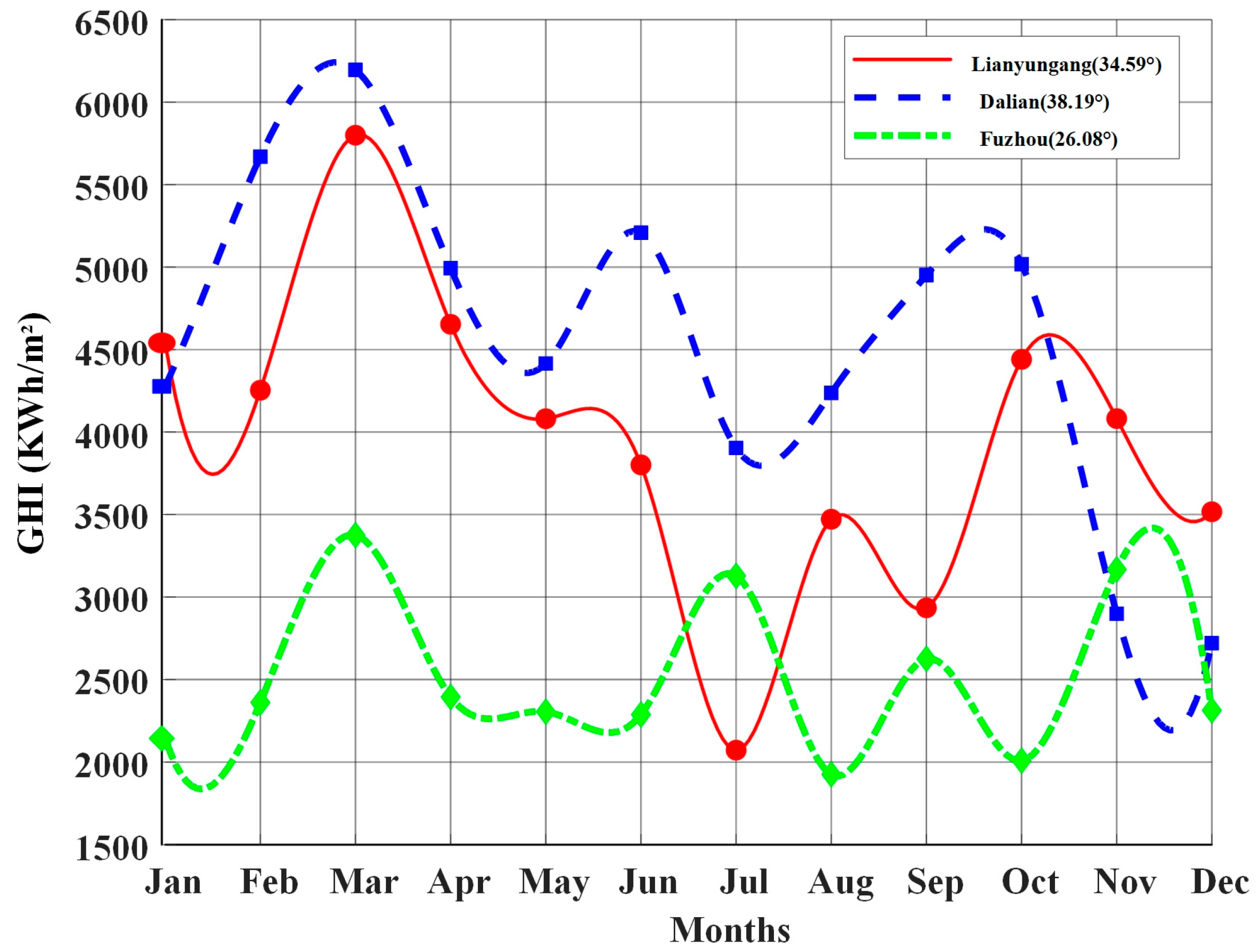
  • Lianyungang City, Jiangsu Province (34.59° N, 119.22° E), located in a temperate monsoon climate zone;
  • Dalian City, Liaoning Province (38.91° N, 121.60° E), characterized by a warm temperate continental monsoon climate;
  • Fuzhou City, Fujian Province (26.08° N, 119.30° E), situated in a subtropical monsoon climate zone.
These sites collectively represent a broad spectrum of solar radiation conditions and seasonal variations across eastern China, providing a robust basis for assessing the adaptability and performance of the optimization algorithm under varying meteorological scenarios.
The meteorological datasets used in this study were obtained from the European Centre for Medium-Range Weather Forecasts (ECMWF), covering the period from January to December 2023 at an hourly temporal resolution. Key variables include the following:
  • Global Horizontal Irradiance (GHI, W/m2);
  • Normal Direct Irradiance ( H b , W/m2);
  • Diffuse Irradiance ( H d , W/m2);
  • Ambient temperature ( T C , °C).
To better represent real-world conditions, this study uses a commercial crystalline silicon PV module as the reference, with key geometric parameters in Table 1. Focusing on geometric effects, the simulation excludes power output modeling and uses annual tilted surface irradiance as the optimization objective. The ground reflectance (albedo) is set to 0.2, representing typical open-field surfaces such as short grass or dry soil. This value lies within the commonly reported range of 0.15–0.25 for natural ground and is widely used as a default in PV modeling when site-specific albedo measurements are not available [48].
Solar irradiance on the tilted surface was calculated using the anisotropic Perez model (Section 2). The three key geometric parameters, tilt angle β , azimuth angle γ , and row spacing D , were jointly optimized via the LO algorithm (Section 4).
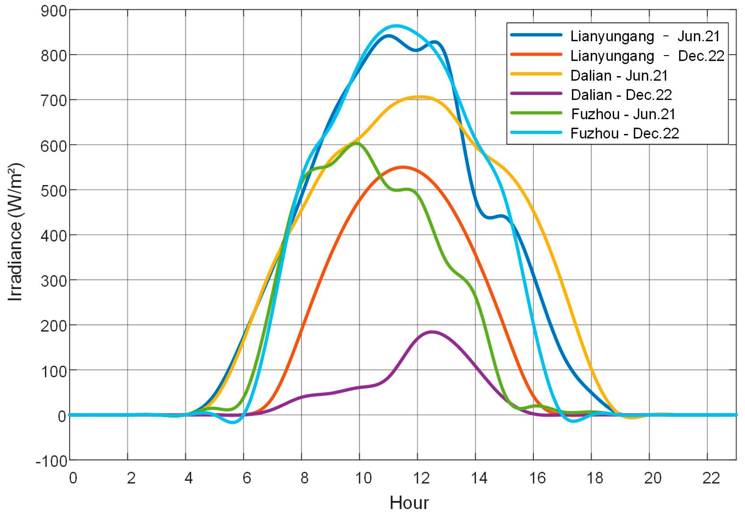
Figure 7 presents the geographical locations of the three selected cities along with their average monthly Global Horizontal Irradiance (GHI) distributions. Figure 8 illustrates the hourly irradiance profiles on representative days for typical seasons in each city, reflecting the variability of solar radiation and providing a basis for assessing the seasonal robustness of the optimization strategy.

4.2. Configurations of the Optimization Model

Numerical implementation and analysis were conducted using MATLAB R2023a. The LO algorithm, a novel swarm intelligence algorithm, balances global search and local exploitation via key hyperparameters. Based on preliminary simulations, this study sets these parameters, as listed in Table 2, to optimize performance and efficiency.
The objective function maximizes the annual total tilted irradiance, calculated by the model f β , γ , D from Section 2. To ensure practical feasibility, the optimization variables are bound based on typical PV installation guidelines:
  • Tilt angle β : 0–90°, covering common ranges for low to mid-latitudes;
  • Azimuth angle γ : −180° to +180°, allowing orientations from southeast to southwest;
  • String spacing D : 2.0–12.0 m, spanning dense to sparse array layouts.
The solution space defined above is as follows:
  β 0 ° , 90 ° ,   γ 180 ° , 180 ° , D 2.0   m , 12.0   m
To simplify the model and focus on the geometric impact on irradiance, the optimization assumes:
  • Single-sided PV modules, ignoring rear-side reflection;
  • No temperature effects on irradiance response;
  • Negligible irregular attenuation from dust, shading, or other factors;
  • Uniform hourly irradiance distribution over the module surface, ignoring transient changes;
  • Ignore component degradation mechanisms such as light-induced degradation (LID) and potential-induced degradation (PID).
  • Constant ground reflectance of 0.2, reflecting typical conditions.
These assumptions reduce variables and improve the clarity and relevance of the results for typical scenarios.

4.3. Simulation Results and Analyses

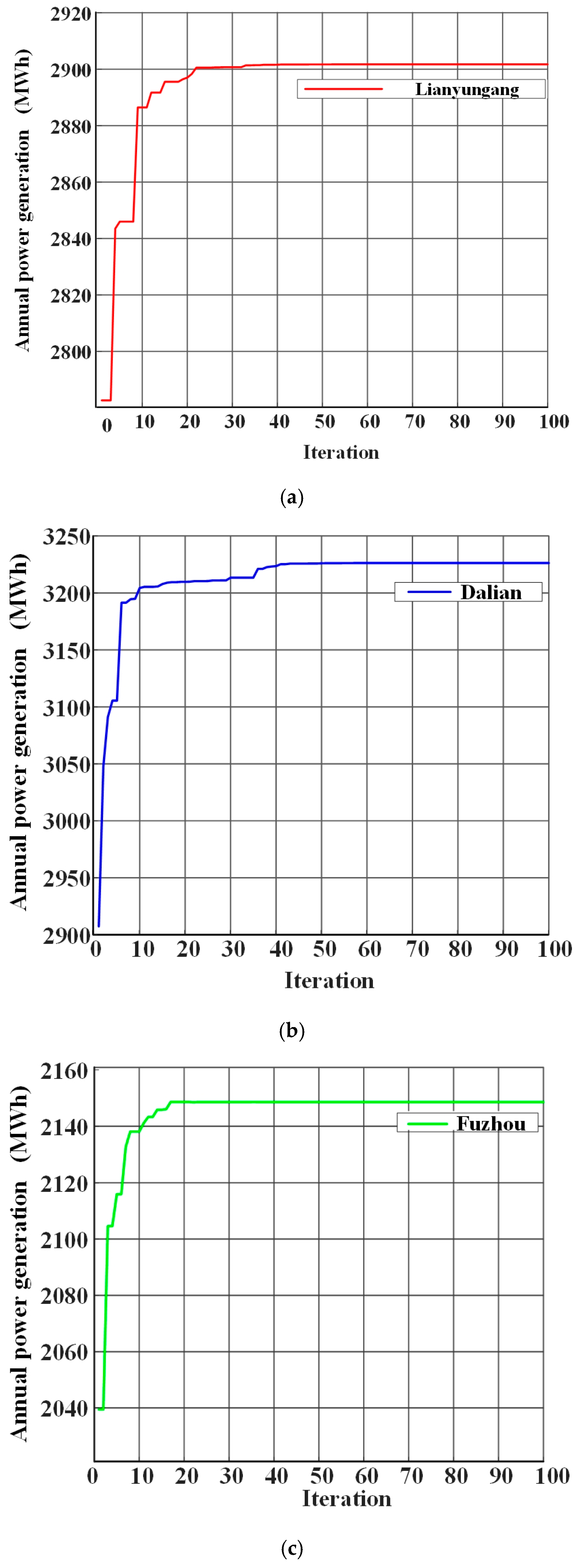
To evaluate the applicability of the LO algorithm for photovoltaic spatial configuration, this study jointly optimizes three parameters: tilt angle β , azimuth angle γ , and row spacing D , aiming to maximize annual total tilted irradiance. The algorithm runs for 100 iterations, recording the best fitness value in each iteration to analyze convergence behavior.
Figure 9 illustrates the convergence trajectories of the LO algorithm for Lianyungang, Dalian, and Fuzhou. In all cases, the fitness value rises sharply during the early iterations, demonstrating strong global exploration capability, and gradually levels off as the algorithm transitions into local exploitation. Lianyungang exhibits the fastest and most stable convergence, reaching a plateau after about 20 iterations with negligible oscillation. Dalian shows a more gradual trajectory, converging around the 40th iteration, while Fuzhou displays smoother but slower improvement, stabilizing after approximately 70 iterations. These convergence behaviors highlight the effectiveness of the LO algorithm: it rapidly identifies promising regions of the search space, refines solutions efficiently, and ultimately stabilizes at consistent optima without significant fluctuations. Moreover, the fact that this stable convergence is observed across three sites with distinct climatic and geographic conditions further underscores the reliability and adaptability of the LO algorithm in photovoltaic layout optimization.
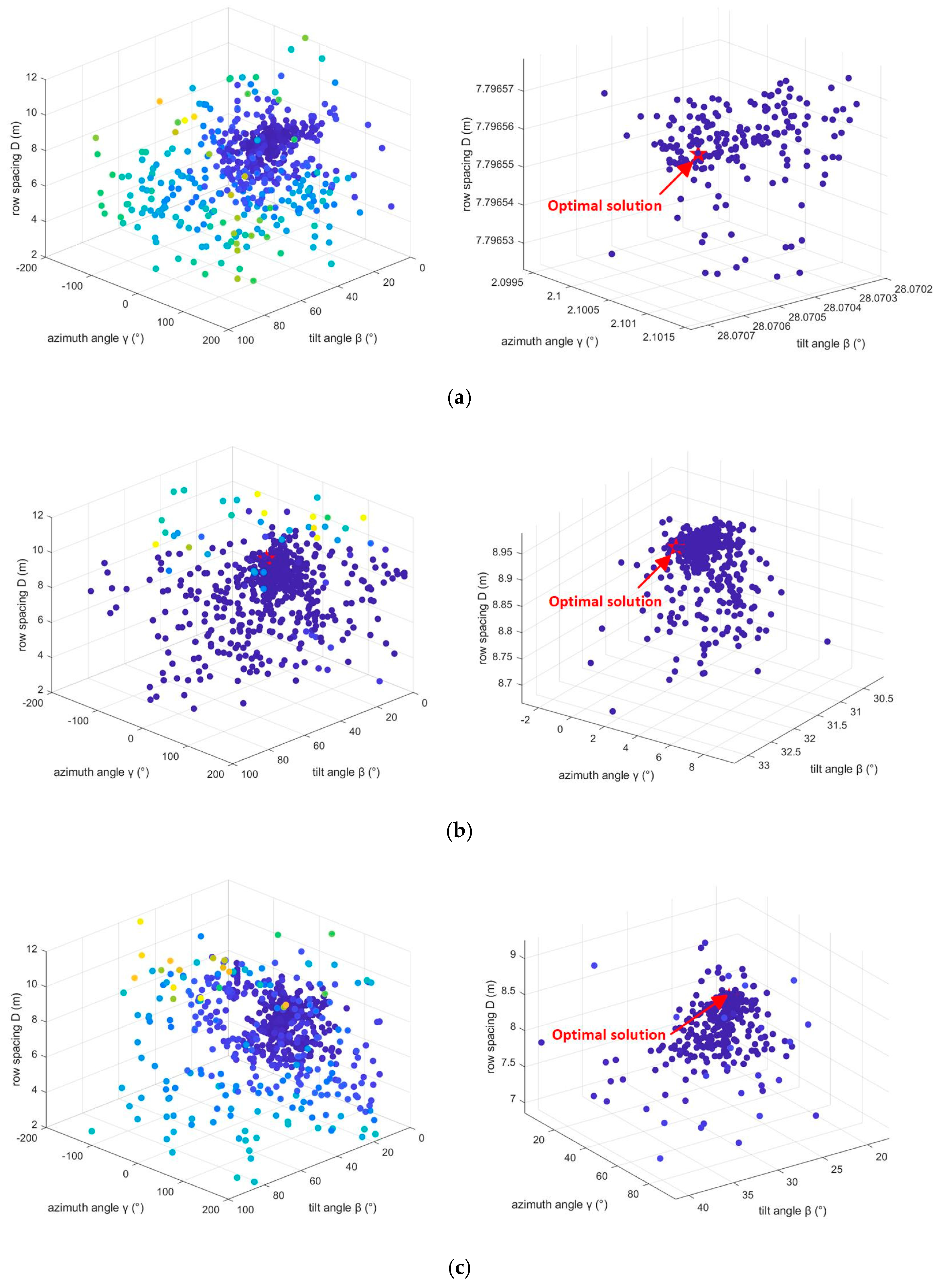
Figure 10 illustrates the optimization solution spaces for Lianyungang, Dalian, and Fuzhou, capturing the complex interactions among the tilt angle β , azimuth angle γ , and row spacing D . For each city, the left panels present the overall distribution of annual energy yield values obtained from candidate configurations evaluated during the LO algorithm search, while the right panels zoom in on the vicinity of the final optimum. In this framework, every candidate β , γ , D is evaluated by calculating its annual energy yield, defined as the sum of hourly PV outputs derived from the Perez transposition model with shading effects and the single-diode PV performance model. During the LO iterations, new candidate solutions are continuously generated through exploration and exploitation operators, and their fitness is compared with existing solutions. At each step, the algorithm preserves the best-so-far solution, ensuring that the final reported optimum is the candidate with the maximum annual energy yield among all solutions explored during the entire optimization process. The optimal configurations, marked with red stars in Figure 10, therefore represent the globally best-performing candidates identified by the LO search. Their location within dense clusters of high-performing solutions demonstrates that the algorithm converges reliably toward robust regions of the solution space. Notably, all three cities exhibit a “saddle-shaped” or clustered high-yield region, underscoring the nonlinear and coupled nature of the design parameters. These spatial characteristics highlight the necessity of simultaneous multi-parameter optimization to effectively balance shading loss and solar energy capture under varying geographic and climatic conditions.
Both the GA and PSO have been widely applied in photovoltaic system optimization problems, particularly for array configuration and layout design, which makes them appropriate baselines for comparison in this study [49,50]. As can be seen from Table 3, after optimizing the spatial layout parameters, the annual total irradiance of Lianyungang, Dalian, and Fuzhou increased significantly without hardware renovation. Compared with the default configuration, all three optimization methods—the GA, PSO, and the proposed LO—achieve consistent performance improvements. Among them, the GA and PSO offer moderate gain, while the LO provides more substantial enhancement. The LO consistently produces the best results at all sites.
Specifically, in Lianyungang, irradiance increased from 2734.81 MWh to 2885.79 MWh (PSO), 2895.44 MWh (GA), and 2901.67 MWh (LO), with respective improvements of 5.52%, 5.87%, and 6.10%, respectively. In Dalian, annual irradiance rose from 2946.51 MWh to 3210.17 MWh (PSO), 3193.64 MWh (GA), and 3226.27 MWh (LO), corresponding to improvements of 8.95%, 8.38%, and 9.49%. Similarly, in Fuzhou, irradiance grew from 2036.59 MWh to 2142.58 MWh (PSO), 2135.42 MWh (GA), and 2148.57 MWh (LO), improving by 3.81%, 5.20%, and 5.50%.
These results confirm that optimizing geometric layout parameters can substantially enhance photovoltaic energy capture under fixed physical conditions. Moreover, the LO algorithm’s stronger global search capability and robustness allow it to outperform both GA and PSO, making it a more efficient and reliable method for PV array optimization across diverse climatic and geographic conditions.
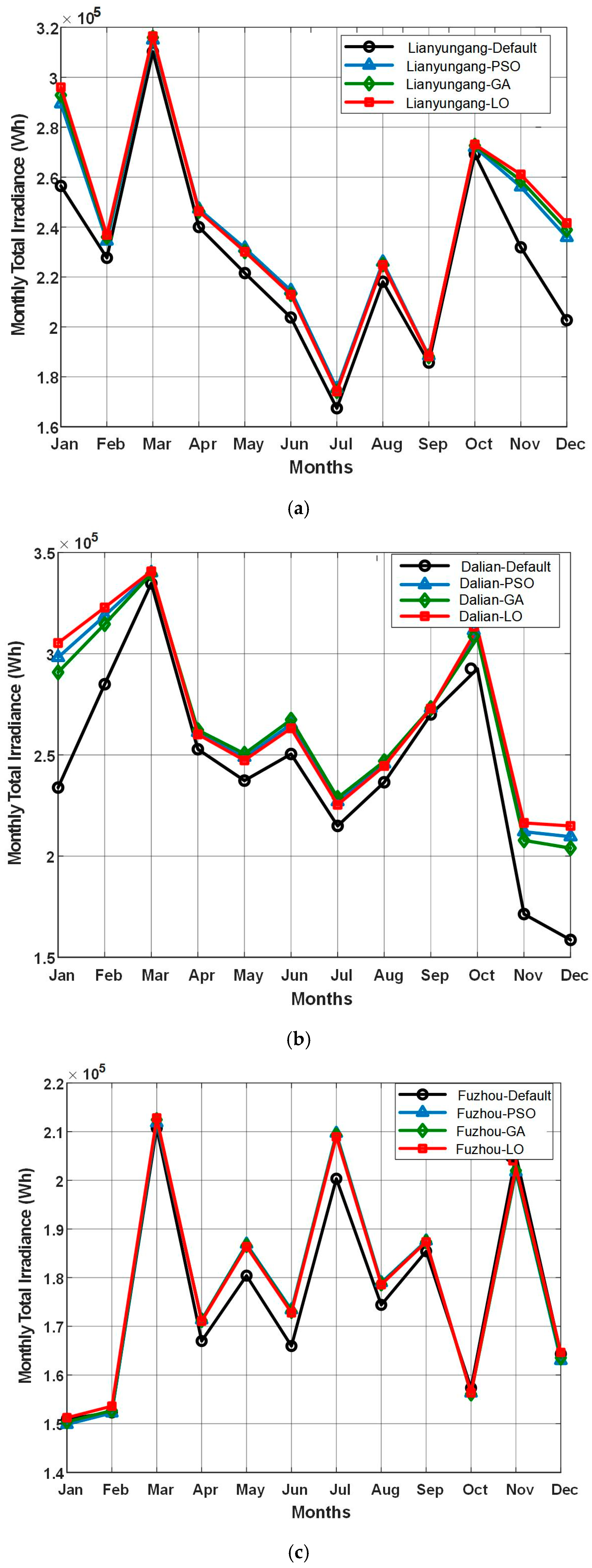
To verify the seasonal adaptability of the proposed optimization strategy, Figure 11 compares the monthly total irradiance of Lianyungang, Dalian, and Fuzhou under default parameters, PSO, GA optimization, and LO. The results show that in most months, the performance of the three optimization algorithms is superior to the default configuration, and LO usually achieves the best performance. It is worth noting that in the months with lower solar altitudes—January, February, November, and December—the irradiance gain usually exceeds 10%, and LO’s compensation for shading and low solar angles is particularly strong. In months with higher solar altitudes, such as June and July, although the default parameters have performed well, both algorithms can still achieve stable improvements. Overall, LO outperforms PSO and the GA in terms of gain amplitude, convergence performance, and adaptability to changes, demonstrating stronger optimization capabilities.
The LO algorithm effectively maximizes the theoretical annual irradiance, highlighting the crucial role of the module geometry in solar capture. The best settings match the environmental conditions: a slight positional shift enhances the collection of direct sunlight throughout the year; a moderate inclination is suitable for the high solar altitude in summer; balanced spacing reduces shading while maintaining land efficiency; and seasonal results show a significant increase in spring and autumn, with enhanced sensitivity to tilt variations, which is consistent with photovoltaic design and solar path principles. All parameters comply with engineering standards and have strong practical potential.
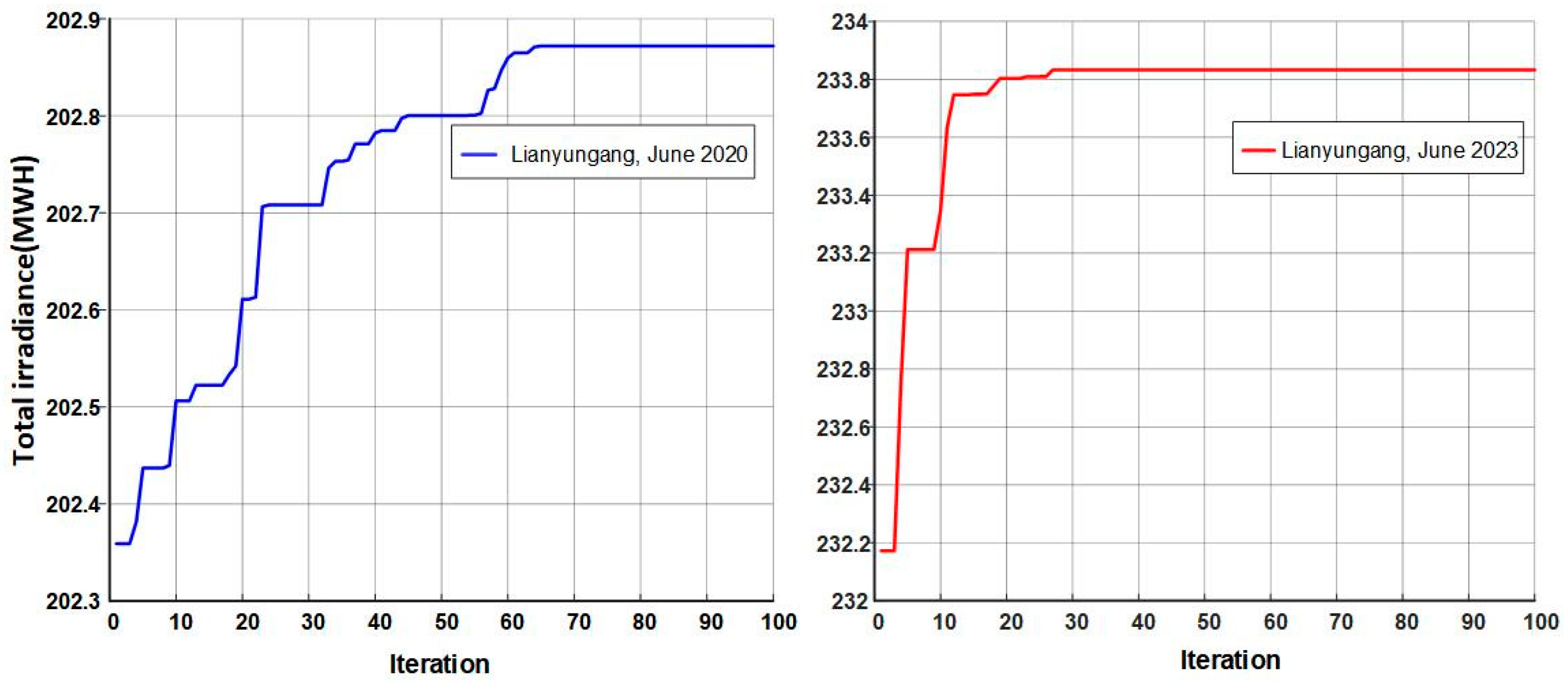
To further verify the robustness of the LO algorithm under meteorological uncertainties, we conducted additional tests using the meteorological datasets of Lianyungang in June 2020 (with frequent rainfall and significantly weakened solar irradiance this month) and June 2023 (with no extreme weather this month, representing a typical climate). The results are shown in Figure 12. The irradiance in June 2020 was significantly lower than that in June 2023, but the LO algorithm still maintained stable convergence behavior, and the fitness curve tended to stabilize within less than 70 iterations. This indicates that although weather conditions reduced absolute irradiance, the LO algorithm reliably identifies the optimal configuration, thereby demonstrating robustness against meteorological uncertainties.

5. Conclusions

This study presents a collaborative optimization strategy for photovoltaic array layout based on the LO algorithm, jointly optimizing tilt angle β , azimuth angle γ , and row spacing D to maximize annual energy yield. The framework integrates the Perez anisotropic irradiance model with hourly geometric shading analysis and incorporates land area, shading loss, and maintenance constraints. The resulting constrained nonlinear problem is solved using the LO algorithm. Case studies in Lianyungang, Dalian, and Fuzhou show that the LO algorithm exhibits superior convergence performance and increases annual energy yield by over 5% in all cases, with a maximum improvement of 9.49% in Dalian. Sensitivity analysis confirms strong nonlinear coupling among β ,   γ , and D emphasizing the need for joint optimization. The results demonstrate the framework’s applicability across diverse climates and locations.
This study has certain limitations that merit acknowledgment. Module degradation mechanisms such as light-induced degradation (LID) and potential-induced degradation (PID) were not explicitly modeled; although these do not affect the short-term comparison of geometric layouts, they may influence long-term performance. In addition, the optimization framework primarily focuses on irradiance-driven energy capture without explicitly incorporating economic indicators such as the Levelized Cost of Electricity (LCOE). Future work will therefore extend the framework by integrating degradation models to evaluate lifetime energy yields more accurately and by embedding economic metrics such as the LCOE into the optimization process. These enhancements will enable the methodology to evolve from purely geometry-driven analysis toward a more comprehensive decision support tool that balances technical performance and economic feasibility, further strengthening its practical relevance.

Author Contributions

All authors contributed to improving the quality of the manuscript. Specifically, G.D. and Y.W. conceptualized the research idea, conducted the theoretical analysis, and performed the experiments. Q.C. and Y.C. contributed to the design of the methodology and experiments, and were actively involved in writing and revising the manuscript. Z.S. and X.L. provided critical feedback on the structure, language, and formatting, and assisted in refining the final version of the paper. All authors have read and agreed to the published version of the manuscript.

Funding

This work was supported by the National Key R&D Project of China under grant No. 2024YFB4206900 and 2024YFB4206901.

Data Availability Statement

The meteorological datasets used in this study were derived from the ERA5 reanalysis dataset provided by the European Centre for Medium-Range Weather Forecasts (ECMWF) and accessed through the Xihe Energy Meteorological Big Data Platform (https://xihe-energy.com/ (accessed on 4 July 2025)).

Conflicts of Interest

The authors declare no conflicts of interest.

References

  1. Yang, B.; Zheng, R.; Han, Y.; Huang, J.; Li, M.; Shu, H.; Su, S.; Guo, Z. Recent Advances in Fault Diagnosis Techniques for Photovoltaic Systems: A Critical Review. Prot. Control Mod. Power Syst. 2024, 9, 36–59. [Google Scholar] [CrossRef]
  2. Li, J.; Zhang, C.; Sun, B. Two-Stage Hybrid Deep Learning with Strong Adaptability for Detailed Day-Ahead Photovoltaic Power Forecasting. IEEE Trans. Sustain. Energy 2023, 14, 193–205. [Google Scholar] [CrossRef]
  3. Chang, Z.; Zhang, A.J.; Wang, H.; Xu, J.; Han, T. Photovoltaic Cell Anomaly Detection Enabled by Scale Distribution Alignment Learning and Multiscale Linear Attention Framework. IEEE Internet Things J. 2024, 11, 27816–27827. [Google Scholar] [CrossRef]
  4. Santos, L.O.; Souza, F.A.; Carvalho Filho, C.O.; Carvalho, P.C.; AlSkaif, T.; Pereira, R.I. Hybrid Modeling for Photovoltaic Module Operating Temperature Estimation. IEEE J. Photovolt. 2024, 14, 488–496. [Google Scholar]
  5. Mignoni, N.; Carli, R.; Dotoli, M. Layout Optimization for Photovoltaic Panels in Solar Power Plants via a MINLP Approach. IEEE Trans. Autom. Sci. Eng. 2025, 22, 18148–18161. [Google Scholar] [CrossRef]
  6. Choi, H.; Choi, J.; Ahn, S.H.; Hyun, J.H.; Cha, H.L.; Lim, B.Y.; Ahn, H.K. Optimal Inclination and Azimuth Angles of a Photovoltaic Module with Load Patterns for Improved Power System Stability. IEEE J. Photovolt. 2024, 14, 525–537. [Google Scholar] [CrossRef]
  7. Zhang, H.; Li, B.; Su, S.F.; Yang, W.; Xie, L. A Novel Hybrid Transformer-Based Framework for Solar Irradiance Forecasting Under Incomplete Data Scenarios. IEEE Trans. Ind. Inform. 2024, 20, 8605–8615. [Google Scholar] [CrossRef]
  8. Dimd, B.D.; Völler, S.; Midtgård, O.M.; Cali, U.; Sevault, A. Quantification of the Impact of Azimuth and Tilt Angle on the Performance of a PV Output Power Forecasting Model for BIPVs. IEEE J. Photovolt. 2024, 14, 194–200. [Google Scholar] [CrossRef]
  9. Sadeghi, R.; Parenti, M.; Memme, S.; Fossa, M.; Morchio, S. A Review and Comparative Analysis of Solar Tracking Systems. Energies 2025, 18, 2553. [Google Scholar] [CrossRef]
  10. Markovics, D.; Mayer, M.J. Comparison of Machine Learning Methods for Photovoltaic Power Forecasting Based on Numerical Weather Prediction. Renew. Sustain. Energy Rev. 2022, 161, 112364. [Google Scholar] [CrossRef]
  11. Saldivar-Aguilera, T.Q.; Valentín-Coronado, L.M.; Peña-Cruz, M.I.; Diaz-Ponce, A.; Dena-Aguilar, J.A. Novel Closed-Loop Dual Control Algorithm for Solar Trackers of Parabolic Trough Collector Systems. Sol. Energy 2023, 259, 381–390. [Google Scholar] [CrossRef]
  12. Blanco, M.J.; Milidonis, K.; Bonanos, A.M. Updating the PSA Sun Position Algorithm. Sol. Energy 2020, 212, 339–341. [Google Scholar] [CrossRef]
  13. Rouholamini, M.; Chen, L.; Wang, C. Modeling, Configuration, and Grid Integration Analysis of Bifacial PV Arrays. IEEE Trans. Sustain. Energy 2021, 12, 1242–1255. [Google Scholar] [CrossRef]
  14. Driesse, A.; Jensen, A.R.; Perez, R. A Continuous Form of the Perez Diffuse Sky Model for Forward and Reverse Transposition. Sol. Energy 2024, 267, 112093. [Google Scholar] [CrossRef]
  15. García, I.; de Blas, M.; Hernández, B.; Sáenz, C.; Torres, J.L. Diffuse Irradiance on Tilted Planes in Urban Environments: Evaluation of Models Modified with Sky and Circumsolar View Factors. Renew. Energy 2021, 180, 1194–1209. [Google Scholar] [CrossRef]
  16. Rynoson, M.; Lu, S.M.; Munkhammar, J.; Campana, P.E. Evaluation of Reverse Transposition and Separation Methods for Global Tilted Irradiance: Insights from High-Latitude Data. Sol. Energy 2025, 297, 113597. [Google Scholar] [CrossRef]
  17. Song, Y.; Huang, L.; Wang, Y.; Du, Y.; Song, Z.; Dong, Q.; Zhao, X.; Qi, J.; Zhang, G.; Li, W.; et al. Energy Performance and Fire Risk of Solar PV Panels under Partial Shading: An Experimental Study. Renew. Energy 2025, 246, 122910. [Google Scholar] [CrossRef]
  18. Mallick, P.; Sharma, R.; Satpathy, P.R.; Thanikanti, S.B.; Nwulu, N.I. A Dimension-Independent Array Relocation (DIAR) Approach for Partial Shading Losses Minimization in Asymmetrical Photovoltaic Arrays. IEEE Access 2023, 11, 63176–63196. [Google Scholar] [CrossRef]
  19. Brecl, K.; Bokalič, M.; Topič, M. Annual Energy Losses Due to Partial Shading in PV Modules with Cut Wafer-Based Si Solar Cells. Renew. Energy 2021, 168, 195–203. [Google Scholar] [CrossRef]
  20. Alcañiz, A.; van Kouwen, M.I.; Isabella, O.; Ziar, H. Wide-Area Sky View Factor Analysis and Fourier-Based Decomposition Model for Optimizing Irradiance Sensors Allocation in European Solar Photovoltaic Farms: A Software Tool. Sol. Energy 2025, 286, 113139. [Google Scholar] [CrossRef]
  21. Kosmopoulos, P.; Dhake, H.; Kartoudi, D.; Tsavalos, A.; Koutsantoni, P.; Katranitsas, A.; Lavdakis, N.; Mengou, E.; Kashyap, Y. Ray-Tracing Modeling for Urban Photovoltaic Energy Planning and Management. Appl. Energy 2024, 369, 123516. [Google Scholar] [CrossRef]
  22. Lofstad-Lie, V.; Marstein, E.S.; Simonsen, A.; Skauli, T. Cost-Effective Flight Strategy for Aerial Thermography Inspection of Photovoltaic Power Plants. IEEE J. Photovolt. 2022, 12, 1543–1549. [Google Scholar] [CrossRef]
  23. Lukač, N.; Mongus, D.; Žalik, B.; Štumberger, G.; Bizjak, M. Novel GPU-Accelerated High-Resolution Solar Potential Estimation in Urban Areas by Using a Modified Diffuse Irradiance Model. Appl. Energy 2024, 353, 122129. [Google Scholar] [CrossRef]
  24. Tripathi, S.; Sahu, H.S.; Kumar, S.; Nayak, S.K.; Mishra, M.K. Maximum Energy Harvest From a TCT Connected PV Array Under Nonhomogeneous Irradiation Conditions. IEEE J. Emerg. Sel. Top. Power Electron. 2023, 11, 5441–5453. [Google Scholar] [CrossRef]
  25. Kim, G.Y.; Han, D.S.; Lee, Z. Solar Panel Tilt Angle Optimization Using Machine Learning Model: A Case Study of Daegu City, South Korea. Energies 2020, 13, 529. [Google Scholar] [CrossRef]
  26. Al-Quraan, A.; Al-Mahmodi, M.; Alzaareer, K.; El-Bayeh, C.; Eicker, U. Minimizing the Utilized Area of PV Systems by Generating the Optimal Inter-Row Spacing Factor. Sustainability 2022, 14, 6077. [Google Scholar] [CrossRef]
  27. Manojkumar, R.; Kumar, C.; Ganguly, S. Optimal Demand Response in a Residential PV Storage System Using Energy Pricing Limits. IEEE Trans. Ind. Inform. 2022, 18, 2497–2507. [Google Scholar] [CrossRef]
  28. Mansour, R.B.; Khan, M.A.M.; Alsulaiman, F.A.; Mansour, R.B. Optimizing the Solar PV Tilt Angle to Maximize the Power Output: A Case Study for Saudi Arabia. IEEE Access 2021, 9, 15914–15928. [Google Scholar] [CrossRef]
  29. Tonita, E.M.; Russell, A.C.; Valdivia, C.E.; Hinzer, K. Optimal Ground Coverage Ratios for Tracked, Fixed-Tilt, and Vertical Photovoltaic Systems for Latitudes up to 75° N. Sol. Energy 2023, 258, 8–15. [Google Scholar] [CrossRef]
  30. Prilliman, M.; Smith, S.E.; Stanislawski, B.J.; Keith, J.M.; Silverman, T.J.; Calaf, M.; Cal, R.B. Technoeconomic Analysis of Changing PV Array Convective Cooling Through Changing Array Spacing. IEEE J. Photovolt. 2022, 12, 1586–1592. [Google Scholar] [CrossRef]
  31. Al Garni, H.Z.; Awasthi, A.; Wright, D. Optimal Orientation Angles for Maximizing Energy Yield for Solar PV in Saudi Arabia. Renew. Energy 2019, 133, 538–550. [Google Scholar] [CrossRef]
  32. Tahir, Z.; Butt, N.Z. Implications of Spatial-Temporal Shading in Agrivoltaics under Fixed Tilt & Tracking Bifacial Photovoltaic Panels. Renew. Energy 2022, 190, 167–176. [Google Scholar] [CrossRef]
  33. McKenna, R.; Mulalic, I.; Soutar, I.; Weinand, J.M.; Price, J.; Petrović, S.; Mainzer, K. Exploring Trade-Offs Between Landscape Impact, Land Use and Resource Quality for Onshore Variable Renewable Energy: An Application to Great Britain. Energy 2022, 250, 123754. [Google Scholar] [CrossRef]
  34. Mayer, M.J. Effects of the Meteorological Data Resolution and Aggregation on the Optimal Design of Photovoltaic Power Plants. Energy Convers. Manag. 2021, 241, 114313. [Google Scholar] [CrossRef]
  35. Ge, Y.; Hu, H.; Chen, J.; Wang, K.; He, Z. Hierarchical Energy Management of Networked Flexible Traction Substations for Efficient RBE and PV Energy Utilization Within ERs. IEEE Trans. Sustain. Energy 2023, 14, 1397–1410. [Google Scholar] [CrossRef]
  36. Awwad, Z.; Alharbi, A.; Habib, A.H.; de Weck, O.L. Site Assessment and Layout Optimization for Rooftop Solar Energy Generation in WorldView-3 Imagery. Remote Sens. 2023, 15, 1356. [Google Scholar] [CrossRef]
  37. Barnawal, P.J.; Lal, V.N.; Singh, R.K. A Dual Half-Active Bridge Resonant Converter for Solar PV Integration Using Grey Wolf Optimization. IEEE Trans. Ind. Appl. 2024, 60, 7087–7097. [Google Scholar] [CrossRef]
  38. Wang, P.; Liang, F.; Song, J.; Jiang, N.; Zhang, X.P.; Guo, L.; Gu, X. Impact of the PV Location in Distribution Networks on Network Power Losses and Voltage Fluctuations with PSO Analysis. CSEE J. Power Energy Syst. 2022, 8, 523–534. [Google Scholar]
  39. Gui, Y.; Nainar, K.; Bendtsen, J.D.; Diewald, N.; Iov, F.; Yang, Y.; Blaabjerg, F.; Xue, Y.; Liu, J.; Hong, T.; et al. Voltage Support With PV Inverters in Low-Voltage Distribution Networks: An Overview. IEEE J. Emerg. Sel. Top. Power Electron. 2024, 12, 1503–1522. [Google Scholar] [CrossRef]
  40. Huang, C.; Zhang, Z.; Wang, L. PSOPruner: PSO-Based Deep Convolutional Neural Network Pruning Method for PV Module Defects Classification. IEEE J. Photovolt. 2022, 12, 1550–1558. [Google Scholar] [CrossRef]
  41. Wittmann, E.; Buerhop-Lutz, C.; Bennett, S.; Christlein, V.; Hauch, J.; Brabec, C.J.; Peters, I.M. PV Polaris—Automated PV System Orientation Prediction. IEEE Photonics J. 2025, 17, 1–7. [Google Scholar] [CrossRef]
  42. Zhang, S.; Niu, D.; Zhou, Z.; Duan, Y.; Chen, J.; Yang, G. Prediction Method of Direct Normal Irradiance for Solar Thermal Power Plants Based on VMD-WOA-DELM. IEEE Trans. Appl. Supercond. 2024, 34, 1–4. [Google Scholar] [CrossRef]
  43. Fang, Y.; Zhao, S.; Du, E.; Li, S.; Li, Z. Coordinated Operation of Concentrating Solar Power Plant and Wind Farm for Frequency Regulation. J. Mod. Power Syst. Clean Energy 2021, 9, 751–759. [Google Scholar] [CrossRef]
  44. Božiková, M.; Bilčík, M.; Madola, V.; Szabóová, T.; Kubík, Ľ.; Lendelová, J.; Cviklovič, V. The Effect of Azimuth and Tilt Angle Changes on the Energy Balance of Photovoltaic System Installed in the Southern Slovakia Region. Appl. Sci. 2021, 11, 8998. [Google Scholar] [CrossRef]
  45. Fan, Y.; Wang, Z.; Wang, J.; Cai, L.; Zhao, B.; Zhou, M.; Li, Q. Evaluation of 12 Transposition Models Using Observations of Solar Radiation and Power Generation. IEEE J. Photovolt. 2022, 12, 444–452. [Google Scholar] [CrossRef]
  46. Niccolai, A.; Grimaccia, F.; Di Lorenzo, G.; Araneo, R.; Ughi, F.; Polenghi, M. A Review of Floating PV Systems With a Techno-Economic Analysis. IEEE J. Photovolt. 2024, 14, 23–34. [Google Scholar] [CrossRef]
  47. Abasi, A.K.; Makhadmeh, S.N.; Al-Betar, M.A.; Alomari, O.A.; Awadallah, M.A.; Alyasser, Z.A.A.; Doush, I.A.; Elnagar, A.; Alkhammash, E.H.; Hadjouni, M. Lemurs Optimizer: A New Metaheuristic Algorithm for Global Optimization. Appl. Sci. 2022, 12, 10057. [Google Scholar] [CrossRef]
  48. Farahat, A.; Kambezidis, H.D.; Kampezidou, S.I. Effect of the Ground Albedo on the Estimation of Solar Radiation on Tilted Flat-Plate Surfaces: The Case of Saudi Arabia. Energies 2023, 16, 7886. [Google Scholar] [CrossRef]
  49. Awad, H.; Salim, K.M.E.; Gül, M. Multi-Objective Design of Grid-Tied Solar Photovoltaics for Commercial Flat Rooftops Using Particle Swarm Optimization Algorithm. J. Build. Eng. 2020, 28, 101080. [Google Scholar] [CrossRef]
  50. Ajmal, A.M.; Ramachandaramurthy, V.K.; Naderipour, A.; Ekanayake, J.B. Comparative Analysis of Two-Step GA-Based PV Array Reconfiguration Technique and Other Reconfiguration Techniques. Energy Convers. Manag. 2021, 230, 113806. [Google Scholar] [CrossRef]
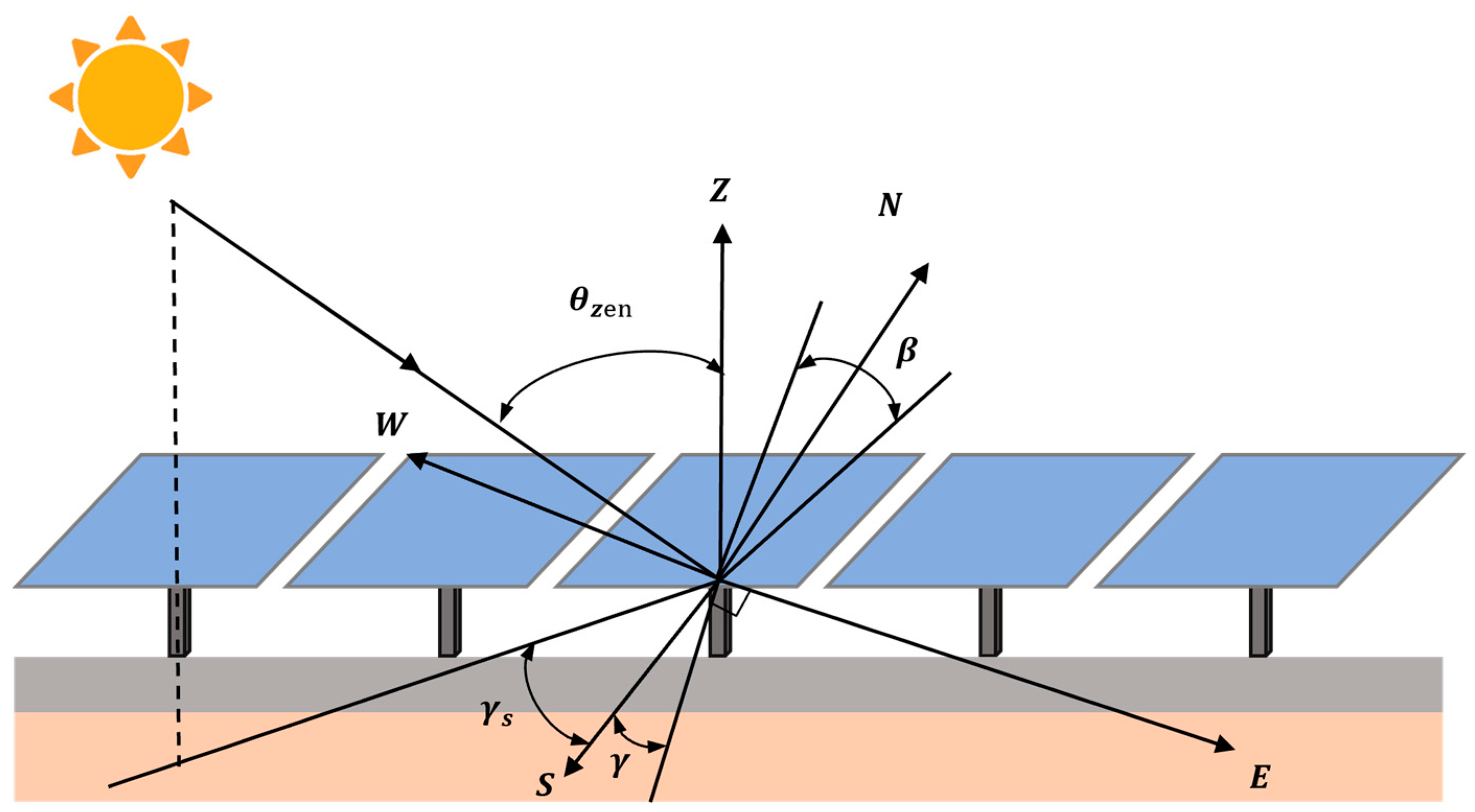
Figure 1. The solar geometry and component orientation diagram adopted in this article. The figure shows the sunlight, component plane, component normal, and geographical orientation for reference.
Symmetry 17 01870 g001
Figure 2. Components of solar radiation received by a tilted PV module.
Symmetry 17 01870 g002
Figure 3. Schematic diagram of unshaded front and rear PV rows.
Symmetry 17 01870 g003
Figure 4. Estimation process of annual total irradiance on the surface of PV modules.
Symmetry 17 01870 g004
Figure 5. Inspiration for the LO algorithm.
Symmetry 17 01870 g005
Figure 6. The optimization process for PV panel tilted-surface irradiance based on the LO algorithm.
Symmetry 17 01870 g006
Figure 7. Monthly average global daily radiation in selected cities.
Symmetry 17 01870 g007
Figure 8. Hourly irradiance variation curves for representative days of typical seasons.
Symmetry 17 01870 g008
Figure 9. Iterative convergence curves of the LO algorithm for selected cities: (a) convergence curve and fitness in Lianyungang; (b) convergence curve and fitness in Dalian; (c) convergence curve and fitness in Fuzhou.
Symmetry 17 01870 g009
Figure 10. Visualization and optimal configuration of the solution space for the selected city. (a) Lianyungang; (b) Dalian; and (c) Fuzhou. Left panel: Candidate dissolution points for sampling (aggregated samples from the iterative process and multiple independent LO runs). Right panel: Optimal solution neighborhood magnification; the red marks represent the final optimal solution.
Symmetry 17 01870 g010
Figure 11. Comparison chart of the three parameter configurations by month: (a) comparison of the three parameter configurations for Lianyungang; (b) comparison of the three parameter configurations for Dalian; (c) comparison of the three parameter configurations for Fuzhou.
Symmetry 17 01870 g011
Figure 12. Robustness verification of the LO algorithm: the left is the convergence curve of Lianyungang in June 2020, representing an uncertain climate, and the right is the convergence curve of Lianyungang in June 2023, representing a typical climate.
Symmetry 17 01870 g012
Table 1. Specification of PV module at standard test conditions.
ParameterValue
Number of PV cells ( n )132
Open circuit voltage ( V o c )44.80 V
Short circuit current ( I s c )18.350 A
Voltage at maximum power point ( V m p )37.70 V
Circuit at maximum power point ( I m p )17.110 A
Maximum power ( P m a x )645 W
Circuit temperature coefficient ( μ s c )9.1 mA/°C
Efficiency of the PV module21.4%
System derating factor10%
Table 2. LO algorithm parameters.
ParameterValue
Lower Bound[0, −180, 2]
Upper Bound[90°, 180°, 12]
Maximum Iterations200
Dimensions3
Low Risk Rate0.1
High Risk Rate 0.5
Table 3. Comparison of annual irradiance under default, PSO, GA and LO optimized parameters.
Selected CityParameter Settings β   ( ° ) γ   ( ° ) D   ( m ) Annual Irradiance (MW)Improvement Magnitude (%)
LianyungangDefault34.5906.002734.81-
PSO26.761.547.202885.79+5.52
GA27.982.307.622895.44+5.87
LO28.072.107.802901.67+6.10
DalianDefault38.1906.002946.51-
PSO30.561.478.203210.17+8.95
GA29.001.767.693193.64+8.38
LO31.821.658.923226.27+9.49
FuzhouDefault26.0806.002036.59-
PSO17.841.636.502142.58+5.20
GA18.212.826.652135.42+4.85
LO18.592.757.162148.57+5.50
Disclaimer/Publisher’s Note: The statements, opinions and data contained in all publications are solely those of the individual author(s) and contributor(s) and not of MDPI and/or the editor(s). MDPI and/or the editor(s) disclaim responsibility for any injury to people or property resulting from any ideas, methods, instructions or products referred to in the content.