Abstract
Air pollution, outstanding particulate matter (PM2.5), poses severe risks to human health and the environment in densely populated urban areas. Accurate short-term forecasting of PM2.5 concentrations is therefore crucial for timely public health advisories and effective mitigation strategies. This work proposes a hybrid approach that combines machine learning models with STL decomposition to provide precise short-term PM2.5 predictions. Daily PM2.5 series from four major Pakistani cities—Islamabad, Lahore, Karachi, and Peshawar—are first pre-processed to handle missing values, outliers, and variance instability. The data are then decomposed via seasonal-trend decomposition using Loess (STL), which explicitly exploits the symmetric and recurrent structure of seasonal patterns. Each decomposed component (trend, seasonality, and remainder) is modeled independently using an ensemble of statistical and machine learning approaches. Forecasts are combined through a weighted aggregation scheme that balances bias–variance trade-offs and preserves the distributional consistency. The final recombined forecasts provide one-day-ahead PM2.5 predictions with associated uncertainty measures. The model evaluation employs multiple statistical accuracy metrics, distributional diagnostics, and out-of-sample validation to assess its performance. The results demonstrate that the proposed framework consistently outperforms conventional benchmark models, yielding robust, interpretable, and probabilistically coherent forecasts. This study demonstrates how periodic and recurrent seasonal structure decomposition and probabilistic ensemble methods enhance the statistical modeling of environmental time series, offering actionable insights for urban air quality management.
1. Introduction
Breathing clean air is essential to human health, as air quality directly impacts the respiratory system and overall well-being. Meteorological and atmospheric factors have a significant impact on air quality and introduce fluctuations in PM2.5 concentrations. Primary NOx, SO2, and VOC emissions combine through photochemical reactions in the presence of sunlight to generate secondary aerosols, while weather factors, including temperature, humidity, and boundary layer height, also affect dispersion. Knowing these mechanisms provides a physical foundation for the temporal patterns. Prolonged exposure to polluted air poses significant health risks beyond the respiratory tract, including increased mortality, the onset of chronic illnesses, disabilities, and substantial socioeconomic burdens on health systems worldwide. Consequently, air quality monitoring and forecasting have become critical components of public health strategies at both national and global levels [1,2,3].
Over the past few decades, rapid population growth, urbanization, and deforestation have contributed to elevated levels of air pollution [4,5,6,7]. Air pollution is generally defined as the presence of harmful chemicals, physical, or biological substances in the atmosphere. Among various pollutants, particulate matter (PM) remains one of the most widely used and reliable indicators of air quality. PM is a complex mixture of solid and liquid particles suspended in the air, often including nitrogen oxides (NOx), carbon oxides (COx), sulfur oxides (SOx), ozone (O3), volatile organic compounds (VOCs), and secondary aerosols. Based on aerodynamic diameter, PM is typically classified into PM10 (particles smaller than 10 µm) and PM2.5 (particles smaller than 2.5 µm) [8].
The health risks associated with particulate matter depend strongly on particle size. PM10 is primarily deposited in the upper respiratory tract and digestive system. By contrast, PM2.5 particles, due to their smaller size, can penetrate deep into the lungs and cross into the bloodstream. This enables them to exert systemic effects, including increased risks of cardiovascular disease, ischemic heart disease, renal disorders, diabetes, and endocrine dysfunctions, as well as neurological conditions such as Alzheimer’s disease, Parkinson’s disease, and multiple sclerosis [9,10]. The World Health Organization (WHO) estimates that exposure to fine particulate matter contributes to approximately 7 million deaths annually, making air pollution one of the leading global health risk factors. In Europe alone, PM2.5 is responsible for nearly 904,000 premature deaths per year, with projections indicating significant increases by 2050 [11]. These alarming statistics underscore the urgency of developing effective monitoring, forecasting, and intervention strategies.
Air pollution dynamics are influenced not only by emissions but also by meteorological and climatic conditions, such as wind speed, temperature, relative humidity, rainfall, atmospheric pressure, and ultraviolet (UV) radiation duration. Consequently, robust air quality monitoring and forecasting systems must integrate both pollution sources and meteorological drivers to provide accurate and reliable predictions [12]. From a probabilistic and statistical perspective, such systems must also capture underlying structures in the data, including symmetries in seasonal patterns, cyclical fluctuations, and approximate symmetry of error distributions.
Pakistan, like many other developing countries, faces significant challenges due to deteriorating air quality. Studies suggest that nearly two-thirds of the country experiences unhealthy air, primarily driven by elevated PM2.5 concentrations, which impose a substantial burden on public health. Respiratory diseases have the most immediate impact, with 57% of chronic obstructive pulmonary disease (COPD) cases and 40% of lower respiratory infections attributed to poor air quality. Beyond respiratory health, prolonged exposure to PM2.5 has also been linked to non-respiratory conditions such as diabetes, cardiovascular disorders, and ischemic heart disease [13]. These findings highlight the need for statistically rigorous and symmetry-aware forecasting frameworks to support evidence-based interventions and policy design.
Air quality forecasting, particularly of PM2.5 concentrations and the Air Quality Index (AQI), has gained significant attention in environmental health research. Accurate forecasts enable the timely issuance of health advisories, informed policy decisions, and the efficient implementation of mitigation strategies. Over the past two decades, a wide range of modeling techniques has been employed, spanning traditional statistical methods (e.g., autoregressive and regression-based models) to advanced machine learning (ML) and deep learning (DL) approaches, each with its own strengths and limitations across different spatiotemporal contexts.
For instance, Mahajan et al. [14] assessed time series forecasting models to predict PM2.5 concentrations in Taichung City, Taiwan. Using hourly data from Air Box microsensor devices, they compared Autoregressive Integrated Moving Average (ARIMA), Neural Network Autoregression (NNAR), and Holt-Winters (HW) models. Based on performance metrics such as the root mean square error (RMSE) and the mean absolute error (MAE), the NNAR model achieved the best predictive accuracy across monitoring stations. Similarly, Mani and Viswanadhapalli [15] investigated AQI forecasting in Chennai, India, using daily data from the Central Pollution Control Board (CPCB) between 2018 and 2020. After applying preprocessing techniques such as missing value imputation and variance stabilization, they demonstrated that ARIMA outperformed multiple linear regression (MLR) in providing stable and reliable forecasts.
In recent years, deep learning methods have emerged as particularly powerful for capturing complex nonlinear dynamics in air quality data. Cassano et al. [16] employed recurrent neural networks (RNNs), including long short-term memory (LSTM) and gated recurrent unit (GRU) architectures, for modeling air quality in Italy’s Apulia region. Leveraging pollutant and meteorological data from the Regional Environmental Protection Agency (ARPA), they demonstrated superior performance of RNNs, particularly in station-specific forecasts. Similarly, Hossain et al. [17] proposed a hybrid GRU–LSTM model for predicting AQI in Dhaka and Chattogram, Bangladesh, based on three years of data (2017–2020). Their hybrid approach consistently outperformed standalone GRU and LSTM models, as measured via a lower RMSE, the MAE, and the mean squared error (MSE). In Beijing, Zhang et al. [18] introduced a hybrid convolutional neural network–LSTM (CNN-LSTM) model that effectively captures both spatial and temporal dependencies, surpassing traditional models such as ARMA, SARIMA, and individual RNN variants.
Efforts to optimize model efficiency have also included the use of advanced machine learning techniques. Liu et al. [19] developed a genetic algorithm-based kernel extreme learning machine (GA-KELM), trained on real-world air quality data from 2019 to 2021. Their model outperformed support vector regression (SVR), Deep Belief Networks (DBN-BP), and the Community Multiscale Air Quality (CMAQ) model in both accuracy and computational speed. However, it required manual tuning of hidden parameters. In the Pakistani context, Iftikhar et al. [20] introduced three ensemble-based models—ESMT, ESME, and ESMV—for AQI forecasting using five years of PM2.5 data from major cities. Their results indicated that ensemble approaches, particularly ESMV, consistently outperformed benchmark models, although the omission of meteorological and gaseous predictors revealed a scope for improvement.
Taken together, these studies reflect a global shift toward hybrid and ensemble modeling approaches in air quality forecasting. From a statistical standpoint, such approaches exploit symmetries in temporal structures (e.g., seasonal recurrences and cyclic regularities) while accommodating asymmetries in pollutant spikes and distributional tails. While traditional models, such as ARIMA and MLR, continue to provide valuable baselines, neural network–based methods—especially those integrating LSTM, GRU, CNN, and optimization algorithms—demonstrate strong potential for addressing the nonlinear and multifaceted nature of air pollution. For environmental health applications, the adoption of symmetry-aware probabilistic and statistical models holds promise for more accurate, interpretable, and actionable forecasts, ultimately supporting improved public health outcomes and sustainable urban air quality management. However, this study defines symmetry as balanced error behavior and recurrent seasonal regularity, rather than as precise temporal symmetry, in contrast to previous works.
The rest of this paper is organized as follows. Section 2 presents the proposed method, including data preprocessing, STL decomposition, ensemble model construction, and the probabilistic–statistical framework for forecasting. Section 3 reports the experimental setup, evaluation metrics, and comparative results with benchmark models, highlighting improvements in accuracy, robustness, and symmetry-based statistical interpretation. Section 4 provides an in-depth discussion of the findings, their implications for environmental health management, and comparisons with prior studies. Finally, Section 6 concludes the paper by summarizing the main contributions, outlining policy implications, and suggesting avenues for future research.
2. Methods and Materials
This study proposes a probabilistic decomposition-based ensemble forecasting framework for predicting daily PM2.5 concentrations in four major Pakistani megacities—Islamabad, Lahore, Karachi, and Peshawar—over a one-day horizon. Rapid variations in emissions, boundary-layer dynamics, and climatic factors influencing short-term dispersion and accumulation are the causes of PM2.5 volatility. The approach is motivated by the theme of symmetry; structural decomposition reveals balanced patterns (trend, seasonality, irregularity), and ensemble integration exploits the complementary strengths of machine learning models through statistical aggregation.
The methodology is organized into three stages: data preprocessing, probabilistic decomposition, and component-wise forecasting with symmetric reconstruction.
- Data Preprocessing: The observed daily PM2.5 concentrations (2019–2023) are preprocessed to ensure reliability. Missing observations are imputed using the Multiple Imputation by Chained Equations (MICE) procedure, which draws imputations from conditional distributions to preserve statistical symmetry and variability in the data (Section 2.1).
- Probabilistic Decomposition: Seasonal-trend decomposition based on Loess (STL) is applied to partition the original series into three additive components: trend (), seasonal (), and remainder (). This decomposition enforces structural decomposition by isolating deterministic and stochastic parts of the signal [21].
- Component Forecasting and Temporal Reconstruction: Each component is independently modeled using four probabilistic machine learning algorithms—support vector regression (SVR), extreme gradient boosting (XGBoost), the Neural Network Autoregressive model (NNETAR), and extreme learning machine (ELM). Their forecasts are symmetrically aggregated to reconstruct the final PM2.5 prediction (Section 2.3).
This design enhances robustness by aligning probabilistic inference with symmetry-based decomposition.
2.1. Multiple Imputation via Chained Equations (MICE)
Let the dataset be , where each variable may contain missing values. The MICE algorithm generates m plausible completed datasets by iteratively imputing missing entries from predictive distributions conditioned on the observed data:
where predictive mean matching (PMM) preserves the distributional consistency between observed and imputed values. The multiple imputations
represent posterior samples, thereby accounting for uncertainty in a symmetric Bayesian framework [22].
2.2. Mathematical Formulation of Forecasting Models
Each decomposed component (, , ) is modeled separately using the following algorithms, with each providing probabilistic estimates respecting data symmetry.
2.2.1. Support Vector Regression (SVR)
SVR constructs a symmetric -insensitive loss function, balancing under- and over-estimation:
Subject to symmetric deviation constraints,
2.2.2. Extreme Gradient Boosting (XGBoost)
XGBoost ensembles regression trees via additive updates under a regularized objective:
where the regularization ensures balanced complexity–fit symmetry.
2.2.3. Neural Network AutoRegressive Model (NNETAR)
NNETAR introduces nonlinear mapping through symmetric activation functions, :
2.2.4. Extreme Learning Machine (ELM)
ELM achieves computational symmetry by randomly assigning input weights and estimating output weights via a pseudoinverse:
In this work, the balanced structural behavior of PM2.5 time series over equivalent temporal intervals is indicated by temporal symmetry. Auto-correlation pattern stability and the almost zero skewness of residuals derived from STL-decomposed components are used to measure symmetry. The directional neutrality between positive and negative forecast deviations is maintained by using point estimates from each model, rather than a weighted aggregate. The theoretical idea of temporal equilibrium in environmental dynamics is reflected in this method’s preservation of structural stability and cyclical regularity.
2.3. Proposed STL–Decomposition Forecasting Framework
By combining point estimates from several base learners, the proposed ensemble framework produces probabilistic projections. The combined outputs capture the uncertainty in model predictions by producing a central tendency (mean forecast).
2.3.1. STL Decomposition
The observed PM2.5 series is decomposed as follows:
with symmetric additive partitioning.
2.3.2. Component Forecasting
For each component and model :
2.3.3. Final Symmetric Reconstruction
The overall PM2.5 forecast is reconstructed by summing the aggregated component forecasts:
This ensures structural symmetry between decomposition and reconstruction.
2.4. Evaluation Metrics
To assess forecasting accuracy, five symmetric and probabilistic metrics are employed (Table 1). These metrics quantify both scale-dependent error (MAE, RMSE) and relative symmetric performance (sMAPE, MDA), while the correlation coefficient r captures probabilistic dependence [23,24,25,26].

Table 1.
Evaluation metrics and their mathematical formulations.
3. Results
Table 2 presents detailed information on the daily PM2.5 datasets collected from four major Pakistani cities—Islamabad, Lahore, Karachi, and Peshawar—covering the period from 2019 to 2023. Each dataset contains 1461 daily entries, ensuring temporal uniformity across locations. The number of observed (non-missing) data points varies slightly, with Islamabad recording 1430, Lahore 1418, Karachi 1426, and Peshawar 1433 valid observations. Consequently, the proportion of missing values remains relatively small, ranging between (Peshawar) and (Lahore). These missing observations were subsequently imputed using the MICE algorithm, which preserves the underlying statistical distribution by generating plausible values from conditional probability models. The low percentage of imputation ensures high data reliability and symmetry of information across all cities, thereby enhancing the robustness of subsequent inferential analysis and comparative modeling.
Table 2.
Details about the datasets considered in this work.
Table 3 provides a comprehensive set of descriptive statistics for each city, including raw values and their logarithmic transformations. All variable units are listed in Table 3; the squared concentration units (µg/m3)2 generate the high variance values, which indicate dispersion, rather than magnitude. The raw distributions reveal heterogeneity across cities: Lahore exhibits the widest range (minimum , maximum ) with the most significant variance () and standard deviation (), suggesting pronounced dispersion and potential outliers. Peshawar records the overall maximum PM2.5 value (), reflecting extreme pollution episodes and elevated variability. In contrast, Islamabad and Karachi exhibit comparatively moderate levels (means of and , respectively) and more minor variances, indicating more stable pollution dynamics. From a probabilistic perspective, skewness and kurtosis statistics highlight the symmetry properties of the distributions. Islamabad and Karachi exhibit relatively balanced distributions (skewness of and , respectively, and kurtosis of and ), indicating near-symmetric patterns with moderate tails. Conversely, Lahore and Peshawar show stronger positive skewness ( and ) and higher kurtosis ( and ), consistent with asymmetric and leptokurtic behavior, where extreme events occur more frequently than in Gaussian processes.
Table 3.
Descriptive statistics of PM2.5 (raw and logarithmic values).
Logarithmic transformation introduces statistical symmetry by stabilizing variance and reducing extreme values, as evidenced by smaller variances and lower dispersion in log-space. The negative skewness of the log-transformed variables further suggests that the transformation mitigates right-skewness, restoring distributional balance. This aligns with the symmetry theme by demonstrating how transformations recover equilibrium in statistical moments and improve interpretability for probabilistic modeling. However, the results of augmented Dickey–Fuller (ADF) and differenced ADF (D_ADF) tests confirm strong stationarity across all series, with test statistics remaining strongly negative. This indicates that the PM2.5 series, once detrended or differenced, attain stable statistical symmetry in their stochastic structure, a crucial prerequisite for time series forecasting.
The concept of symmetry, central to the theme of this study, is examined both statistically and temporally within the PM2.5 time series. From a statistical perspective, symmetry refers to the balanced distribution of concentration values around the central tendency. To assess this property, descriptive statistics such as Figure 1 present seasonal subseries plots to evaluate temporal symmetry in PM2.5. Karachi and Peshawar show inconsistencies later captured in the STL remaining components, while Lahore and Islamabad show a moderately similar pattern due to the occurrence of high-pollution episodes. However, the application of logarithmic transformation substantially reduces skewness and excess kurtosis across all cities, thereby improving the symmetry of the distributions. This enhanced statistical symmetry stabilizes the variance and mitigates the influence of outliers, improving the performance of subsequent machine learning models.
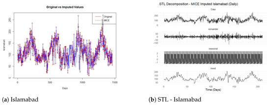
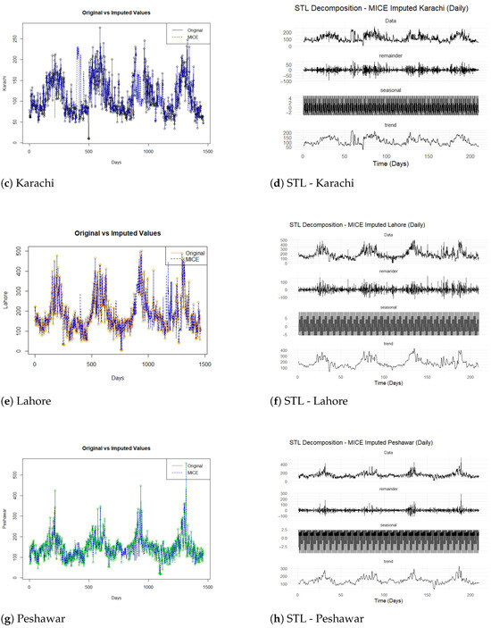
Figure 1.
Comparison of original and STL-decomposed PM2.5 series for four cities.
From a temporal perspective, symmetry manifests through the repetitive, cyclic patterns captured via the STL decomposition (Figure 1). The seasonal component exhibits a nearly symmetric oscillation around the long-term trend, reflecting recurring emission cycles and meteorological regularities. The decomposition thereby isolates symmetric temporal fluctuations from irregular residual variations, which enables more interpretable and stable forecasting. In addition, the proposed STL-based hybrid framework exploits these symmetrical characteristics through its ensemble design. Models with distinct inductive biases—SVR and ELM for linear relationships, and NNAR for nonlinear dynamics—are integrated to maintain equilibrium between underfitting and overfitting tendencies. This balanced modeling structure effectively enforces a probabilistic form of symmetry in the error distribution, as reflected in the nearly unbiased residuals and improved directional accuracy (MDA) across all cities. Collectively, these findings confirm that both statistical and temporal symmetry are intrinsic to the PM2.5 series and are strategically leveraged within the proposed hybrid framework to enhance predictive precision and interpretability.
In air quality, temporal symmetry refers to recurrent seasonal or diurnal patterns that exhibit steady structural repetition throughout time. Figure 1 presents seasonal subseries plots to evaluate temporal symmetry in PM2.5: Karachi and Peshawar show inconsistencies later captured in the STL remaining components, while Lahore and Islamabad show moderate similar pattern. A comparative assessment of the original and MICE-imputed time series of PM2.5 concentrations for the four major cities, Islamabad, Karachi, Lahore, and Peshawar, together with their corresponding STL decompositions, is provided in Figure 1. The imputed series, as displayed in Figure 1a,c,e,g, exhibit a high degree of concordance with the original data, successfully preserving underlying temporal patterns and abrupt fluctuations. This alignment demonstrates that the MICE procedure accurately restored missing values while maintaining the statistical symmetry of the series, i.e., the balance between smooth cyclic components and irregular stochastic variations. Notably, the imputation preserved the integrity of extreme values in more volatile environments such as Lahore and Peshawar, where sudden pollution spikes are characteristic of episodic urban activity and meteorological shocks. However, the term “volatile environments” refers to urban contexts characterized by high temporal variability and abrupt fluctuations in PM2.5 concentrations, typically driven by short-term anthropogenic and meteorological influences such as irregular industrial emissions, traffic congestion peaks, biomass burning, dust storms, and temperature inversions. Notably, the imputation preserved the integrity of extreme values in such volatile environments, particularly in Lahore and Peshawar—where sudden pollution spikes reflect episodic urban activity and meteorological shocks. In contrast, relatively stable environments like Islamabad exhibit smoother and more symmetric seasonal cycles with limited short-term disturbances. Recognizing these differences is essential, as hybrid ensemble models must adapt to both symmetric and asymmetric fluctuation patterns to maintain forecasting accuracy across diverse urban conditions.
The subsequent STL decompositions, shown in Figure 1b,d,f,h, further validate the reliability of the imputation step. In each case, the decomposition successfully disentangled the trend, seasonal, and remainder components, ensuring that the structural symmetry between long-term drift, cyclic oscillations, and irregular shocks was preserved. Islamabad and Lahore reveal smooth seasonal cycles and steady trend evolution, suggesting symmetric and stable temporal dynamics. By contrast, Karachi and Peshawar exhibit greater short-term variability, implying asymmetries introduced via external factors such as industrial activity or meteorological dispersion effects.
Taken together, these results confirm that the MICE-based imputation not only filled missing values without distorting the temporal structure but also maintained the probabilistic and structural symmetry required for reliable downstream modeling. The preservation of trend–seasonal balance and the accurate representation of extreme events ensures that the reconstructed series provides a statistically consistent foundation for subsequent hybrid ensemble forecasting of PM2.5 concentrations. However, it is acknowledged that validating the imputation using the same dataset may not provide a fully independent measure of reliability. Therefore, in this study, the evaluation of MICE-imputed PM2.5 values emphasizes internal consistency, rather than external validation. Specifically, we assessed the reliability of the imputation by comparing the statistical distributions, temporal dynamics, and decomposed STL components between the original and imputed series. The close alignment of these characteristics suggests that the MICE procedure effectively preserves the intrinsic temporal and probabilistic structure of the data without introducing artificial bias. Nevertheless, future studies could further strengthen imputation validation by employing external datasets, such as concurrent meteorological observations or adjacent monitoring station records, to independently assess imputation fidelity.
3.1. Islamabad
For Islamabad, several statistical indicators—MAE, RMSE, correlation, sMAPE, and MDA—were employed to evaluate the STL-decomposed forecasting frameworks. The comparative results, summarized in Table 4, reveal that the four leading hybrid configurations were as follows: {SVRt + ELMr + NNARs}, {NNARt + ELMr + NNARs}, {ELMt + ELMr + NNARs}, and {XGBt + ELMr + NNARs}. Among these, the {SVRt + ELMr + NNARs} model emerged as the most effective, attaining the lowest sMAPE (7.56) and RMSE (7.91), the highest MDA (0.838), and a strong correlation (0.969). This balanced performance illustrates its ability to capture both the symmetry of forecast alignment and probabilistic directional consistency. The near-identical accuracy of the second- and third-ranked models, {NNARt + ELMr + NNARs} and {ELMt + ELMr + NNARs}, highlights the robustness of ELM and NNAR integration. Finally, the {XGBt + ELMr + NNARs} specification also performed competitively (RMSE: 7.99; correlation: 0.969), underscoring the utility of boosting strategies for trend representation. Overall, these findings confirm that statistical symmetry between error minimization and directional forecasting can be effectively achieved using ensemble architectures.
Table 4.
Islamabad: accuracy mean error.
3.2. Karachi
For Karachi, a consistent performance pattern emerges across STL-based hybrid configurations, as detailed in Table 5. The top four models were identified as follows: {ELMt + ELMr + NNARs}, {NNARt + ELMr + NNARs}, {SVRt + ELMr + NNARs}, and {XGBt + ELMr + NNARs}. For the most effective among these, {ELMt + ELMr + NNARs}, the lowest RMSE (7.652) and MAE (6.005) were reported, together with a favorable sMAPE (7.590) and high correlation (0.975). By employing ELM for both trend and residual components and NNAR for seasonality, this model effectively balanced nonlinear and linear dynamics, reflecting probabilistic symmetry in capturing both smooth cycles and stochastic fluctuations. The next two models, {NNARt + ELMr + NNARs} and {SVRt + ELMr + NNARs}, attained slightly higher RMSE values but exhibited identical correlation (0.975) and MDA (0.798), demonstrating equivalent directional symmetry. The {XGBt + ELMr + NNARs} model also achieved stable correlation and MDA scores, though with modestly higher error magnitudes. These outcomes reinforce the effectiveness of combining statistical learning algorithms (ELM, SVR, NNAR, XGBoost) in decomposition-based hybrid structures for air quality forecasting.
Table 5.
Karachi: accuracy mean error.
3.3. Lahore
In Lahore, model evaluation emphasized RMSE due to its sensitivity to large deviations, which is particularly relevant, given the volatility of PM2.5 levels in the region. As reported in Table 6, the {ELMt + ELMr + NNARs} configuration yielded the lowest RMSE (12.475), alongside the lowest MAE (10.120) and sMAPE (8.340). Despite exhibiting a slightly lower MDA (0.808) than its nearest rival, this model demonstrated probabilistic superiority by consistently reducing both absolute and relative forecast errors. The second-best specification, {SVRt + ELMr + NNARs}, achieved a competitive RMSE (12.521), while recording the highest MDA (0.818) and a correlation of 0.979. This indicates enhanced directional symmetry despite marginally higher error variance. The other contenders, {XGBt + ELMr + NNARs} and {NNARt + ELMr + NNARs}, posted RMSE values of 12.556 and 12.819, respectively, but they retained comparable correlation and MDA values. Collectively, these results highlight the probabilistic trade-off between minimizing error magnitudes and maximizing directional alignment, reinforcing the reliability of ELM-based ensemble schemes in volatile urban environments.
Table 6.
Lahore: accuracy mean error.
3.4. Peshawar
For Peshawar, four STL-hybrid frameworks, each employing SVR for the residual component, were evaluated (Table 7). The leading model, {SVRt + SVRr + NNARs}, reported the lowest RMSE (13.585), MAE (10.871), and a competitive sMAPE (9.902), confirming its accuracy in capturing both absolute and relative forecast structures. The {ELMt + SVRr + NNARs} variant achieved a nearly identical RMSE (13.620) and MAE (10.898) while outperforming in terms of MDA (0.779), suggesting enhanced directional symmetry despite slightly higher error levels. The remaining specifications, {NNARt + SVRr + NNARs} and {XGBt + SVRr + NNARs}, achieved RMSE scores of 13.621 and 13.651, respectively, but they did not surpass the SVR-dominated frameworks in error minimization. These findings demonstrate that using SVR consistently for both trend and residual components yields robust probabilistic accuracy, while NNAR contributes additional symmetry in capturing seasonality.
Table 7.
Peshawar: accuracy mean error.
A comparative visualization of original (imputed) and predicted PM2.5 levels for the four cities is presented in Figure 2. For Islamabad (Figure 2a), forecasts nearly overlap with the imputed series, showing symmetric alignment with seasonal cycles. Karachi (Figure 2b) exhibits higher short-term variability; the models slightly underestimate extreme spikes but capture the general probabilistic distribution. In Lahore (Figure 2c), high oscillations and peak concentrations reveal a challenge in capturing extreme values, highlighting the asymmetry introduced by outliers. Finally, Peshawar (Figure 2d) demonstrates the accurate detection of a significant concentration peak, indicating strong responsiveness to abrupt shifts. Taken together, the results suggest that the models exhibit statistical symmetry and robustness in relatively stable contexts (Islamabad, Peshawar). In contrast, adaptive or hybrid refinements are necessary for more volatile settings (Lahore, Karachi) to enhance extreme-value representation and probabilistic reliability.
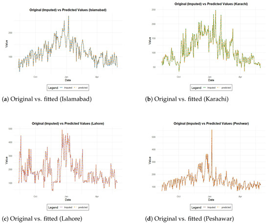
Figure 2.
Original vs. fitted PM2.5 values for four monitoring stations.
4. Discussion
This study used four machine learning algorithms to compare the imputed (actual) and forecasted PM2.5 concentrations in four major Pakistani cities: Peshawar, Lahore, Karachi, and Islamabad. SVR, ELM, NNAR, and XGBoost were used in the proposed hybrid framework. Performance measures, including RMSE, MAE, MAPE, correlation, sMAPE, and time series plots (actual vs. predicted), were used to empirically and visually assess the efficiency of these models. Additionally, this section presents the best-performing PM2.5 forecasting model proposed via this study, which is evaluated in detail and compared to baseline methods and the best models found in the literature. To enhance air quality predictions and management, this section also outlines potential avenues for future research and provides practical policy recommendations.
4.1. Comparative Studies with Benchmark Models and Existing Literature
To assess the robustness and practical relevance of the proposed hybrid forecasting framework, a comparative evaluation against four widely used benchmark models—support vector regression (SVR), extreme gradient boosting (XGBoost), neural network autoregression (NNAR), and extreme learning machine (ELM)—was conducted across the four urban centers of Islamabad, Karachi, Lahore, and Peshawar. The performance was examined using a comprehensive suite of accuracy metrics, including the mean absolute error (MAE), the root mean squared error (RMSE), Pearson correlation, the symmetric mean absolute percentage error (sMAPE), and the mean directional accuracy (MDA). These measures collectively capture both point-wise accuracy and directional predictive reliability, thereby addressing the probabilistic and distributional symmetry underlying forecast errors.
Table 8 presents a detailed comparative analysis. In Islamabad, the proposed model demonstrates substantial improvements over conventional baselines, achieving an RMSE of 7.912 and a high correlation of 0.969, compared with the nearest competing model (ELM), which yields an RMSE of 21.563 and a correlation of only 0.667. This reflects the ability of the proposed hybrid decomposition–ensemble strategy to capture symmetric seasonal patterns and reduce asymmetric error deviations, thereby yielding more reliable forecasts. Similarly, in Karachi, where pollution exhibits dynamic fluctuations, the proposed model attains an RMSE of 7.652 and an exceptionally high correlation of 0.975. This outperformance demonstrates how the hybrid model maintains structural balance between the trend and remainder components, aligning with the symmetry properties inherent to complex urban time series.
Table 8.
Comparative performance of the proposed hybrid framework versus benchmark models across four Pakistani cities.
Lahore poses the most challenging forecasting environment due to its highly volatile and heterogeneous PM2.5 patterns. While benchmark models yield inconsistent results and a larger dispersion of errors, the proposed approach achieves an RMSE of 12.475 and a correlation coefficient of 0.979. The symmetric formulation of sMAPE in this case is particularly valuable, as it penalizes over- and under-predictions in a balanced manner, underscoring the framework’s superior capability to model asymmetric distributions. In Peshawar, despite extreme episodes of pollution, the proposed model again exhibits resilience, recording an RMSE of 13.585 and a correlation coefficient of 0.837, while also achieving the highest MDA, highlighting its predictive stability in the face of directional changes.
A broader comparison with the existing literature suggests that classical machine learning models (e.g., SVR, XGBoost) often fail to capture the nonlinearities and seasonal symmetries inherent to PM2.5 series, resulting in higher error magnitudes and reduced correlation. By contrast, the proposed hybrid approach systematically integrates decomposition, statistical learning, and ensemble weighting to exploit both temporal symmetry and probabilistic consistency. The consistent superiority across all four cities confirms the model’s adaptability, interpretability, and robustness. Additionally, our methodology makes sure that positive and negative errors are treated equally, but this shouldn’t be taken as finding temporal symmetry. Decomposition and ensemble integration, not symmetry characteristics, are responsible for the benefits. More importantly, the integration of symmetric error metrics, such as sMAPE and balanced correlation analysis, aligns with the objectives of the Symmetry special issue, illustrating how probabilistic and statistical perspectives on symmetry enhance predictive performance and strengthen decision-making in urban air quality management. The hybrid STL–ensemble technique provides a data-driven approach to managing urban air quality while improving forecasting accuracy and interpretability overall.
4.2. Comparative Analysis with Prior Studies
Beyond the benchmark comparisons, the performance of the proposed hybrid STL-based forecasting framework was evaluated against results reported in prior studies on PM2.5 prediction. This additional comparison provides a broader perspective on its relative efficiency and highlights how probabilistic and statistical considerations of symmetry in forecast errors contribute to improved accuracy.
An ensemble technique reported in [20] using the same dataset achieved RMSE values of 20.32, 48.31, 22.99, and 35.06 for Islamabad, Lahore, Karachi, and Peshawar, respectively. By contrast, the proposed hybrid model achieved significantly lower RMSEs of 7.91, 12.48, 7.65, and 13.59 for the same cities. These results represent error reductions of approximately 61%, 74%, 67%, and 61%, respectively, demonstrating the proposed framework’s capacity to capture underlying structural patterns with a higher degree of symmetry and reduced variability in forecast deviations.
Similarly, in [27], the reported RMSE values were 16.566 (Islamabad), 20.835 (Lahore), 22.084 (Karachi), and 18.743 (Peshawar). When compared to the proposed model, which obtained RMSEs of 7.912, 12.475, 7.652, and 13.585, the reductions were to 52%, 40%, 65%, and 28%, respectively. These improvements indicate not only higher predictive accuracy but also a more stable and symmetric distribution of residuals, which is critical for enhancing generalization across heterogeneous urban air quality contexts.
In another study, ref. [28] employed an artificial neural network (ANN) with 20 neurons and five independent variables to predict PM2.5 in Islamabad, obtaining an RMSE of 9.82. By comparison, the proposed STL-based model, which relies solely on intrinsic PM2.5 dynamics without exogenous predictors, achieved a lower RMSE of 7.912, representing a 19% improvement. This reinforces the advantage of decomposition-based models in capturing temporal symmetries without heavy reliance on external covariates.
Furthermore, ref. [29] utilized ANN models incorporating meteorological and historical information, producing RMSE values of 18 for Karachi and 39 for Lahore. In contrast, the proposed model achieved RMSEs of 7.652 and 12.475 for Karachi and Lahore, respectively, representing improvements of over 57% and 68%. This outcome emphasizes the robustness of the proposed approach in capturing both short-term fluctuations and the seasonal symmetries inherent in PM2.5 data.
A more advanced deep learning approach in [30], which integrated CNN-LSTM with Multi-Fractal Detrended Fluctuation Analysis (MF-DFA), reported an RMSE of 11.732 using combined meteorological and air quality data. While effective, the proposed hybrid STL-based framework still outperformed this model, achieving an average RMSE of 10.91 across the four cities, despite utilizing only the PM2.5 series as input. This highlights the effectiveness of decomposition and ensemble strategies in enhancing forecast precision while preserving statistical symmetry in error dynamics.
Therefore, the comparative evidence across diverse studies consistently demonstrates the superiority of the proposed framework in terms of error reduction, robustness, and adaptability. By integrating decomposition, ensemble learning, and symmetric error measures such as sMAPE, the approach systematically balances over- and under-predictions, reduces asymmetry in residual distributions, and achieves higher probabilistic consistency. Additionally, meteorological factors like temperature, humidity, and wind speed are out of this study, although this design decision improves the models’ applicability in low-resource settings where such data are difficult to obtain or inconsistent. Future iterations of the suggested framework, however, might include these exogenous factors to investigate how they affect the interpretability and accuracy of the model.
5. Policy Implications and Future Studies
The implications of this work extend beyond methodological contributions to environmental policy, public health, and sustainable urban management. Accurate short-term forecasts of PM2.5 concentrations are crucial for issuing timely health advisories, managing traffic, emission control, and implementing regulatory interventions. For urban planners, such forecasts can inform land-use strategies, infrastructure development, and mitigation policies aimed at reducing long-term exposure to hazardous pollutants. The demonstrated reliability of the proposed framework across multiple cities underscores its scalability for nationwide deployment. Unlike models that require extensive meteorological datasets, this decomposition–ensemble method provides a cost-effective and practical solution for resource-constrained regions, such as Pakistan. When integrated into regulatory monitoring systems, the model can enhance compliance mechanisms, improve environmental governance, and foster evidence-based decision-making.
Despite its strong performance, several avenues for future research remain open. Incorporating exogenous covariates, such as meteorological conditions, socioeconomic activity, or industrial emissions, could further enhance predictive accuracy, particularly during extreme pollution episodes. Additionally, by adding external covariates, sophisticated symmetry measures, and Bayesian-based probabilistic augmentation, future studies could expand this symmetry-aware ensemble, and exploring alternative decomposition techniques such as Variational Mode Decomposition (VMD), Complete Ensemble Empirical Mode Decomposition with Adaptive Noise (CEEMDAN), or Empirical Wavelet Transform (EWT) may capture asymmetries and nonlinearities more effectively in highly volatile environments. Extending the model toward probabilistic forecasting frameworks could also quantify uncertainty, providing policymakers with confidence intervals and risk assessments, rather than point estimates. In conclusion, the proposed hybrid ensemble model represents a statistically rigorous, symmetry-aware, and interpretable solution for urban air quality forecasting. Its adaptability, accuracy, and efficiency make it a valuable tool for policymakers, environmental researchers, and urban planners seeking proactive, data-driven approaches to sustainable air quality management.
6. Conclusions
This study has introduced a novel hybrid ensemble framework for forecasting PM2.5 concentrations in four major Pakistani cities—Islamabad, Lahore, Karachi, and Peshawar—by leveraging seasonal—trend decomposition using Loess (STL) in combination with support vector regression (SVR), an extreme learning machine (ELM), and neural network autoregression (NNAR). The probabilistic and statistical synergy between decomposition and ensemble modeling enabled the framework to capture both linear and nonlinear dynamics while preserving the temporal symmetry of the underlying air quality processes. The empirical evaluation demonstrated that the proposed approach consistently achieved superior forecasting performance compared to benchmark models, such as SVR, XGBoost, ANN, and CNN—LSTM. With an average RMSE of 10.91 across all locations, the model outperformed the prior literature, including CNN—LSTM—MF—DFA (RMSE 11.73) and traditional ANN-based systems (RMSEs above 18 and 39 for Karachi and Lahore, respectively). The reduction in error ranged from 40% to 65%, underscoring both the robustness and efficiency of the proposed model. Importantly, these results were achieved without incorporating exogenous meteorological covariates, highlighting the model’s capacity to operate in data-constrained environments. The decomposition of the PM2.5 series into trend, seasonal, and remainder components enhanced interpretability by revealing the probabilistic balance and structural symmetry between persistent trends, cyclic variations, and irregular shocks. Visual diagnostics and statistical accuracy measures confirmed that the hybrid ensemble not only reduced errors but also improved directional accuracy, thereby reinforcing its practical relevance. Overall, this study contributes to the literature on environmental forecasting by demonstrating how probability-driven decomposition and symmetry-aware hybridization can lead to both accuracy and interpretability in complex time series modeling. In addition to offering a reliable and understandable method for short-term PM2.5 forecasting, the framework may be expanded to include other environmental time series.
Author Contributions
Conceptualization, methodology, and software, H.I.; validation, H.I., A.F.H., M.Q., and P.C.R.; formal analysis, H.I. and A.F.H.; investigation, H.I., A.F.H., M.Q., and P.C.R.; resources, M.Q., A.F.H. and P.C.R.; data curation, H.I. and M.Q.; writing—original draft preparation, H.I., A.F.H., M.Q., and P.C.R.; writing—review and editing, H.I., M.Q., P.C.R., and A.F.H.; visualization, A.F.H., P.C.R., and M.Q.; supervision, P.C.R. and H.I.; project administration, A.F.H. and P.C.R.; funding acquisition, A.F.H. and P.C.R. All authors have read and agreed to the published version of the manuscript.
Funding
This work was supported and funded by the Deanship of Scientific Research at Imam Mohammad Ibn Saud Islamic University (IMSIU) (grant number IMSIU-DDRSP2502).
Data Availability Statement
The data used in this study are available at https://www.iqair.com/pakistan (accessed on 20 June 2024).
Conflicts of Interest
The authors declare no conflicts of interest.
References
- Maio, S.; Sarno, G.; Tagliaferro, S.; Pirona, F.; Stanisci, I.; Baldacci, S.; Viegi, G. Outdoor air pollution and respiratory health. Int. J. Tuberc. Lung Dis. 2023, 27, 7–12. [Google Scholar] [CrossRef] [PubMed]
- Wu, C.; Wang, R.; Lu, S.; Tian, J.; Yin, L.; Wang, L.; Zheng, W. Time-Series Data-Driven PM2.5 Forecasting: From Theoretical Framework to Empirical Analysis. Atmosphere 2025, 16, 292. [Google Scholar] [CrossRef]
- Li, J.; Liang, L.; Lyu, B.; Cai, Y.S.; Zuo, Y.; Su, J.; Tong, Z. Double Trouble: The Interaction of PM2.5 and O3 on Respiratory Hospital Admissions. Environ. Pollut. 2023, 338, 122665. [Google Scholar] [CrossRef]
- Destiartono, M.E.; Hartono, D. Does Rapid Urbanization Drive Deforestation? Evidence From Southeast Asia. Econ. Dev. Anal. J. 2022, 11, 442–453. [Google Scholar]
- Oyetunji, P.; Ibitoye, O.; Akinyemi, G.; Fadele, O.; Oyediji, O. The effects of population growth on deforestation in Nigeria: 1991–2016. J. Appl. Sci. Environ. Manag. 2020, 24, 1329–1334. [Google Scholar] [CrossRef]
- Song, J.; Ma, C.; Ran, M. AirGPT: Pioneering the Convergence of Conversational AI with Atmospheric Science. NPJ Clim. Atmos. Sci. 2025, 8, 179. [Google Scholar] [CrossRef]
- Liu, Y.; Chen, B.; Zheng, Y.; Cheng, L.; Li, G.; Lin, L. ODMixer: Fine-Grained Spatial-Temporal MLP for Metro Origin-Destination Prediction. IEEE Trans. Knowl. Data Eng. 2025, 37, 5508–5522. [Google Scholar] [CrossRef]
- Harrison, R.M. Airborne particulate matter. Philos. Trans. R. Soc. A 2020, 378, 20190319. [Google Scholar] [CrossRef]
- Kyung, S.Y.; Jeong, S.H. Particulate-matter related respiratory diseases. Tuberc. Respir. Dis. 2020, 83, 116. [Google Scholar] [CrossRef]
- Pryor, J.T.; Cowley, L.O.; Simonds, S.E. The physiological effects of air pollution: Particulate matter, physiology and disease. Front. Public Health 2022, 10, 882569. [Google Scholar] [CrossRef]
- Tarín-Carrasco, P.; Im, U.; Geels, C.; Palacios-Peña, L.; Jiménez-Guerrero, P. Contribution of fine particulate matter to present and future premature mortality over Europe: A non-linear response. Environ. Int. 2021, 153, 106517. [Google Scholar] [CrossRef] [PubMed]
- Zhang, Y. Dynamic effect analysis of meteorological conditions on air pollution: A case study from Beijing. Sci. Total Environ. 2019, 684, 178–185. [Google Scholar] [CrossRef]
- Fatima, M.; Butt, I.; Nasar-u Minallah, M.; Atta, A.; Cheng, G. Assessment of air pollution and its association with population health: Geo-statistical evidence from Pakistan. Geogr. Environ. Sustain. 2023, 16, 93–101. [Google Scholar] [CrossRef]
- Mahajan, S.; Chen, L.J.; Tsai, T.C. An empirical study of PM2.5 forecasting using neural network. In Proceedings of the 2017 IEEE SmartWorld, Ubiquitous Intelligence & Computing, Advanced & Trusted Computed, Scalable Computing & Communications, Cloud & Big Data Computing, Internet of People and Smart City Innovation (SmartWorld/SCALCOM/UIC/ATC/CBDCom/IOP/SCI), San Francisco, CA, USA, 4–8 August 2017; IEEE: New York, NY, USA, 2017; pp. 1–7. [Google Scholar]
- Mani, G.; Viswanadhapalli, J.K.; Stonier, A.A. Prediction and forecasting of air quality index in Chennai using regression and ARIMA time series models. J. Eng. Res. 2022, 10, 179–194. [Google Scholar] [CrossRef]
- Cassano, F.; Casale, A.; Regina, P.; Spadafina, L.; Sekulic, P. A recurrent neural network approach to improve the air quality index prediction. In Ambient Intelligence–Software and Applications–, 10th International Symposium on Ambient Intelligence; Springer: Cham, Switzerland, 2020; pp. 36–44. [Google Scholar]
- Hossain, E.; Shariff, M.A.U.; Hossain, M.S.; Andersson, K. A novel deep learning approach to predict air quality index. In Proceedings of the International Conference on Trends in Computational and Cognitive Engineering: Proceedings of TCCE 2020; Springer: Singapore, 2020; pp. 367–381. [Google Scholar]
- Zhang, J.; Li, S. Air quality index forecast in Beijing based on CNN-LSTM multi-model. Chemosphere 2022, 308, 136180. [Google Scholar] [CrossRef]
- Liu, C.; Pan, G.; Song, D.; Wei, H. Air quality index forecasting via genetic algorithm-based improved extreme learning machine. IEEE Access 2023, 11, 67086–67097. [Google Scholar] [CrossRef]
- Iftikhar, H.; Qureshi, M.; Zywiołek, J.; López-Gonzales, J.L.; Albalawi, O. Short-term PM2.5 forecasting using a unique ensemble technique for proactive environmental management initiatives. Front. Environ. Sci. 2024, 12, 1442644. [Google Scholar] [CrossRef]
- Wen, Q.; Gao, J.; Song, X.; Sun, L.; Xu, H.; Zhu, S. RobustSTL: A robust seasonal-trend decomposition algorithm for long time series. In Proceedings of the AAAI Conference on Artificial Intelligence, Honolulu, HI, USA, 27 January–1 February 2019; Volume 33, pp. 5409–5416. [Google Scholar]
- Van Buuren, S.; Groothuis-Oudshoorn, K. mice: Multivariate imputation by chained equations in R. J. Stat. Softw. 2011, 45, 1–67. [Google Scholar] [CrossRef]
- Iftikhar, H.; Zafar, A.; Turpo-Chaparro, J.E.; Canas Rodrigues, P.; López-Gonzales, J.L. Forecasting Day-Ahead Brent Crude Oil Prices Using Hybrid Combinations of Time Series Models. Mathematics 2023, 11, 3548. [Google Scholar] [CrossRef]
- Aamir, M.; Iftikhar, H.; Nasir, J.; Rodrigues, P.C.; Alharbi, A.A.; Allohibi, J. A Novel Hybrid LMD-SPF Forecasting Framework for Financial Time Series: Evidence from Gold Returns. AIMS Math. 2025, 10, 21875–21901. [Google Scholar] [CrossRef]
- Cuba, W.M.; Huaman Alfaro, J.C.; Iftikhar, H.; López-Gonzales, J.L. Modeling and Analysis of Monkeypox Outbreak Using a New Time Series Ensemble Technique. Axioms 2024, 13, 554. [Google Scholar] [CrossRef]
- Carbo-Bustinza, N.; Iftikhar, H.; Belmonte, M.; Cabello-Torres, R.J.; De La Cruz, A.R.H.; López-Gonzales, J.L. Short-Term Forecasting of Ozone Concentration in Metropolitan Lima Using Hybrid Combinations of Time Series Models. Appl. Sci. 2023, 13, 10514. [Google Scholar] [CrossRef]
- Ahmed, M.; Xiao, Z.; Shen, Y. Estimation of ground PM2.5 concentrations in Pakistan using convolutional neural network and multi-pollutant satellite images. Remote Sens. 2022, 14, 1735. [Google Scholar] [CrossRef]
- Sadiq, N.; Uddin, Z. Modeling of PM2.5 concentrations using artificial neural networks: A case study of Islamabad. Glob. NEST J. 2024, 27, 06865. [Google Scholar]
- Sadiq, N.; Uddin, Z. Prediction of PM2.5 via precursor method using meteorological parameters. EQA-Int. J. Environ. Qual. 2025, 67, 45–50. [Google Scholar]
- Pak, U.; Kim, H.; Jong, U.; Hyon, R.; Kim, J.; Kim, K.; Kim, K. A deep learning approach via multifractal detrended fluctuation analysis for PM2.5 prediction. J. Atmos. Sol.-Terr. Phys. 2025, 268, 106444. [Google Scholar] [CrossRef]
Disclaimer/Publisher’s Note: The statements, opinions and data contained in all publications are solely those of the individual author(s) and contributor(s) and not of MDPI and/or the editor(s). MDPI and/or the editor(s) disclaim responsibility for any injury to people or property resulting from any ideas, methods, instructions or products referred to in the content. |
© 2025 by the authors. Licensee MDPI, Basel, Switzerland. This article is an open access article distributed under the terms and conditions of the Creative Commons Attribution (CC BY) license (https://creativecommons.org/licenses/by/4.0/).