Asymptotic Symmetry Behavior for a Sampled Data Model via Fractional-Order Hold and Delta Operators

Abstract

Controllers designed on the basis of an approximate discrete time model can fail when they are applied to the real processes. This is a problem of interest in adaptive symmetry control system theory. In this paper, we introduce the certain polynomial for discretizing the $n$-th order integrator in the case of a fractional-order hold (FROH) and delta operator. Moreover, the corresponding FROH discretization pulse transfer function and sampling data model in normal form are derived. On the basis of these results, we present FROH discrete system zero dynamics and sampling zero dynamics where their asymptotic symmetry properties are obtained. In addition, the implications incorporating sampling zero dynamics in the discrete-time models used for system identification become evident as the sampling period approaches zero. It is a further extension of the corresponding results.

1. Introduction

Many, and arguably most, physical adaptive symmetry control systems are described by continuous-time ordinary differential equation models. However, in actual process, these models need to be discretely sampled first. The sampled-data system, also known as the computer control system, contains both continuous-time signals and discrete-time signals, i.e., sampled signals [1,2]. The sampled-data model is obtained by deriving the corresponding continuous-time system after discretization. Therefore, researchers sought to extend the correlation results of the continuous system model to the sampled-data model. Symmetry is the invariance (unchanging nature) of a system under a transformation, such as rotation, reflection, or translation. It represents balance, order, and conservation. However, since the structure of the sampling symmetry model is much more complex than that of a continuous system, some information in the continuous control system is lost during the sampling process [3], and the theory of the continuous system model is far more mature than the theory of the discrete sampling model. Thus, the adaptive sampled-data model is of interest to the majority of scholars [4,5,6,7].

The zero (dynamics) and pole play important roles in the design of the control system. The presence of unstable zero-poles limits the control performance that the adaptive control system achieves. When a continuous-time system is discretized by the sampling switch and the holder, there is a simple correspondence between the corresponding continuous-time pole and the discrete-time pole. If there is an unstable zero in the process or object, it is difficult to build an adaptive control system [8]. Thus, it can be expected that there is a definite formula, such as the pole, to describe the mapping between the zero of the continuous-time system and that of the discrete system, or at least an approximate description. Since the zero of the discrete system is a function of the sampling period, it is difficult to derive this description of the relationship, and it is possible to describe the zero characteristic only in some special cases. Therefore, under the limit that the sampling interval vanishes, research on the zero characteristics of adaptive symmetry discrete systems has attracted widespread attention from researchers [9,10,11,12,13].

In the adaptive control of discrete time or sampled data, signal reconstruction devices are indispensable. Therefore, in the discussion of the adaptive symmetry discrete sampling model and zero characteristic, the signal reconstruction device mainly considers the use of zero-order hold (ZOH). The famous Swedish scholar Åström et al. [9] conducted a groundbreaking study of the adaptive discrete-time system model and its zero-point feature in 1984, which described the discrete-time model of a single-input single-output (SISO) system with a ZOH. When the sampling period approaches zero, the zero point of the discrete time is called the limiting zero point. According to Åström et al., the limiting zero point includes the intrinsic zero and the sampling zero. The former corresponds to the zero of the continuous-time system; the latter is determined by the relative degree of the corresponding continuous-time system and the number of original continuous-time zeros and converges to the roots of some specific polynomials [14].

In much of the discussion about the properties of adaptive discrete-time zeros, the ZOH has been employed mainly as a hold circuit since it is used most commonly in practice. For example, Ishitobi et al. [10] analyzed the zeros of the sampled-data models corresponding to continuous-time decouplable multi-input multi-output systems with all relative degrees less than or equal to two and showed approximate expressions of the zeros as power series expansions with respect to a sampling period. Moreover, stability criteria for the zeros for small sampling periods are given. Taking into account the fact that the type of hold circuit used critically influences the position of zeros, it is an interesting problem to investigate the zeros in the case of various holds, such as a first-order hold (FOH) [15], fractional-order hold (FROH) [11], etc. In the case of the FOH, there is no advantage over ZOH in terms of the stability of zeros of the resulting discrete-time systems. However, as an alternative to the ZOH, the FROH can locate the zeros of the discrete-time system inside the unit circle in some cases when the ZOH fails to do so. The FROH was proposed by Philips and Nagle [16]. It is an extension of the FOH and is also called the generalized FOH. FROH holds the signal amplitude at its input and adds to it a signal proportional to the difference between the present and past sampled amplitudes, i.e., the first difference. The key attempt to study the FROH was made by Passino and Antsaklis [17], who described the asymptotic behavior of the discrete-time zero dynamics for a fast sampling rate, as the original continuous-time plant is discretized with an FROH. According to this fundamental attempt, these two researchers considered the FROH as an alternative to the ZOH and showed that it can locate the zero dynamics of a discrete-time system inside the unit circle in some cases when the ZOH fails to do so. Ishitobi [18] analyzed the stability properties and derived the stability conditions of the limiting zero dynamics when the continuous-time systems have a relative degree of up to five for sufficiently small sampling periods. In that paper, it was proven that the FROH leads to inversely stable discretized plants for a wider class of continuous-time systems with a relative degree of two. Further results on the advantages of the FROH have been reported by Bàrcena and collaborators [19,20,21,22]. They discuss the limiting zero dynamics—as the sampling period tends to zero—of sampled systems composed of an FROH, a continuous-time plant and a sampler in cascade. Moreover, the FROH circuit and neural network techniques are proposed in these manuscripts to manage a computer hard disk read/write head described as a second-order system. In addition, Rubio et al. [23,24] presented a discrete-time model reference control for practical milling via FROH discretization. For multi-input multi-output systems, the result of the stability properties of the limiting zero dynamics of discrete-time multivariable systems with FROHs was reported by Liang et al. [25]. In addition, the influence of time delays on digital control systems must be considered because of their existence. Liang et al. [26] and Zeng et al. [27] analyzed the stability of the limiting zero dynamics of discrete-time systems corresponding to continuous-time systems with a time delay when FROH is used for signal reconstruction and presented the stability conditions of the limiting zero dynamics of discrete-time systems for time delay systems with a delay. On the other hand, Ishitobi and Nishi [28,29] proposed an approximate sampled-data model for the nonlinear system in the case of an FROH. In addition, their results demonstrate that the limiting zeros corresponding to continuous-time zeros are located at 1 and that the remaining limiting zeros are situated at the points with the specific constant values determined by some definite polynomials. Furthermore, if the corresponding continuous zero is stable, the zero of the former case approaches 1 from inside the unit circle as the sampling period tends to 0. Moreover, some zeros of the latter case reach −1 and there remains the possibility that they approach the unit circle from inside. The previous work does not provide any answer to this question. Our manuscript analyzes the asymptotic properties of discretization sampling zeros such that the purpose of this paper is to provide an answer to this question. When the zero of the desired sampled-data system decreases from inside the unit circle to −1, the sampling period tends to zero. The result is derived by expressing the value of the zero as a function of a sampling period. This approach is useful because it extends the application area of adaptive symmetry control. Moreover, when the $q$ operator and the delta operator are used to sample the continuous-time system, the delta operator has better control performance than the $q$ operator in tracking the continuous-time system. That is to say, the discrete sampling model in the case of the delta operator is closer to its original continuous-time system than the previous results. Hence, our manuscript has focused on the extensive application of the delta operator, which enables a more explicit and coherent connection between a sampled-data model and its underlying continuous-time system.

On the other hand, since different signal reconstruction devices affect the position of the zero point, it is necessary to expand the study of the adaptive symmetry discrete sampling system model and its zero position distribution on the basis of different signal holders. In this paper, we will study the two types of adaptive symmetry sampled-data models in the case of the FROH. Under the condition of the holder, that is, the standard description of the discretization pulse function and the discrete sampling models, and further, the adaptive asymptotic properties and approximate expressions of the zero dynamics for corresponding FROH, adaptive discretization systems are explored. Moreover, the sampling zero dynamics for nonlinear plants are identical to those found in the linear case. This paper also investigates the implications incorporating these sampling zero dynamics into discrete-time nonlinear models used for system identification. Finally, we compare the different system identifications based on the discrete sampling output observations and their zero characteristics.

The remainder of this paper is structured as follows: In Section 2, we review known results for adaptive sampled linear systems, using the delta operator. The n-th order integrator discretization models and their asymptotic behaviors are represented in Section 3. In Section 4, the primary findings of this paper are as follows: zero dynamics and system identification of the sampled-data models for nonlinear systems. Finally, conclusions are presented in Section 5.

Regarding the contributions of our manuscript, we believe that three aspects will make it interesting to general researchers of the sampled-data system with a fractional-order hold (FROH). First, we introduce the certain polynomial of discretizing the n-th order integrator in the case of an FROH and delta operator. Also, the corresponding FROH discretization pulse transfer function and sampling data model in normal form are derived. On the basis of these results, we present FROH discrete system zero dynamics and sampling zero dynamics where their asymptotic properties are obtained. In addition, the implications of including these sampling zero dynamics in the discrete-time models are represented as the sampling period tends to zero.

2. Preparatory Knowledge and Theoretical Basis

Digital computers have become an indispensable part of modern industrial control systems. All of the current modern adaptive control systems are actually based on computer-controlled discrete sampling systems. It is usually composed of a sampling switch, a signal holder and a continuous-time system, which contains two steps: sampling and holding, namely, the sampling of the continuous-time signal and the reconstruction of the discrete-time signal into a continuous time signal.

In the control of discrete sampling, signal reconstruction devices are indispensable for sampling or holding the sampler and retainer throughout the digital adaptive control system. Since the different signal reconstruction devices will affect the position of the zeros for the discrete sampling systems, the ZOH and FROH signal reconstruction devices are now introduced.

ZOH is the most commonly used and simplest sampling signal holder, which is a constant value extrapolated retainer, and keeps the sample value $u\left(kT\right)$ in the previous time $kT$ intact to the next sampling time $\left(k+1\right)T$; when the next sampling time $\left(k+1\right)T$ arrives, the sampled value becomes $u\left(\left(k+1\right)T\right)$, and the extrapolation is continued by the sample value. In other words, the sample value of $kT$ can only hold to a sampling period $T$, and immediately drop to zero until the next sampling time arrival; The output of ZOH is

$$u\left(t\right)=u\left(kT\right), kT\le t\le \left(k+1\right)T, k=1,2,\cdots$$

(1)

The transfer function of ZOH can be expressed as

$$G_{ZOH}\left(s\right)={\displaystyle \frac{1-e^{-Ts}}{s}}$$

(2)

FROH is an extension of the FOH. It is also called the generalized first-order hold. FROH holds the signal amplitude at its input and adds to it a signal proportional to the difference between the present and past sampled amplitude the first difference. It has also been extrapolated on the basis of the values of two sampling moments, and its extrapolated output t is the time variable between one and the other. The output of FROH can be described as

$$\begin{array}{ll}u\left(t\right)=u\left(kT\right)+\beta & \left[{\displaystyle \frac{u\left(kT\right)-u\left(\left(k-1\right)T\right)}{T}}\right]\left(t-kT\right)\\ & kT\le t\le \left(k+1\right)T, k=1,2,\dots \end{array}$$

(3)

where $\beta$ is a proportional factor. The FOH is extrapolated on the basis of the values of two sampling moments, and its extrapolated output t is the time variable between A and B, the output of FOH can be described as

$$\begin{array}{ll}u\left(t\right)=u\left(kT\right)+& {\displaystyle \frac{u\left(kT\right)-u\left(\left(k-1\right)T\right)}{T}}\left(t-kT\right)\\ & kT\le t\le \left(k+1\right)T, k=1,2,\dots \end{array}$$

(4)

Obviously, the ZOH and FOH can be referred to a particular case of the FROH when $\beta =0$ and $\beta =1$, respectively. The transfer function of FROH can be expressed as

$$G_{FROH}\left(s\right)=\left(1-\beta e^{-Ts}\right){\displaystyle \frac{1-e^{-Ts}}{s}}+{\displaystyle \frac{\beta }{T{s}^2}}{\left(1-e^{-Ts}\right)}^2$$

(5)

The majority of the results and textbooks on discrete-time systems usually describe the models using the shift operator $q$ and the associated ${\rm Z}$-transform. The shift operator $q$ is called the forward transfer operator, i.e., $qf\left(k\right)=f\left(k+1\right)$, which plays an important role in the connection to the continuous-time system and its corresponding discrete sampling model [5,7,9,10,11,12]. Compared with the shift operator $q$, the sampling discrete-time model of the delta operator $\delta$ is closer to the original continuous-time system [3,4]. The relationship between a sampled-data model and the underlying continuous-time system can be better expressed by the use of the delta operator, both in the discrete time domain and complex variable domain [6]:

$$\delta ={\displaystyle \frac{q-1}{T}}\iff \gamma ={\displaystyle \frac{z-1}{T}}$$

(6)

where $z$ and $\gamma$ are the complex variables involved in the $q$ and $\delta$ domains, respectively, and where $T$ is the sampling period. The use of the $\delta$-operator corresponds to a reparameterization of sampled-data models, enabling explicit inclusion of the sampling period in their discrete-time description.

The zero point and the pole contain the basic characteristics of the control system. The zero point reflects the coupling relationship between the internal variable and the input and output, and the pole reflects the internal coupling and the autonomous characteristic of the system. For a continuous system, consider its corresponding transfer function:

$$G\left(s\right)={\displaystyle \frac{F\left(s\right)}{E\left(s\right)}}$$

(7)

where the eigenvalues of polynomials $F\left(s\right)$ and $E\left(s\right)$ represent the zero and pole of the continuous-time control system, respectively, and the concrete expression is as follows:

$$\left\{\begin{array}{c}F\left(s\right)=C{\left(s{I}_n-A\right)}^{\ast }B=\det \left[\begin{array}{cc}s{I}_n-A& -B\\ C& 0\end{array}\right]\\ E\left(s\right)=\det \left(s{I}_n-A\right)\end{array}\right.$$

(8)

where $\ast$ is the adjoint matrix.

For the discrete sampling system model, when the $q$ operator is used, the transfer function of the corresponding discrete sampling model is

$$G_q\left(z\right)=C{\left(z{I}_n-A_q\right)}^{-1}{B}_q={\displaystyle \frac{F_q\left(z\right)}{E_q\left(z\right)}}$$

(9)

for which

$$\left\{\begin{array}{c}{F}_q\left(z\right)=C{\left(z{I}_n-A_q\right)}^{\ast }{B}_q=\det \left[\begin{array}{cc}z{I}_n-A_q& -B_q\\ C& 0\end{array}\right]\\ E_q\left(z\right)=\det \left(z{I}_n-A_q\right)\end{array}\right.$$

(10)

In Equations (9) and (10), the roots of polynomials $F_q\left(z\right)$ and $E_q\left(z\right)$ represent the zero and pole of the discrete sampling control system, respectively. Among them, there is a one-to-one exponential relationship between the poles of the continuous-time system and the poles of the corresponding discrete sampling model. That is:

The pole of $G\left(s\right)$ (eigenvalues ${\lambda }_i$ of $A$)

$\Rightarrow$ the pole of $G_q\left(z\right)$ (eigenvalues $e^{{\lambda }_{i}T}$ of $A_q$)

The relationship between the zero of the continuous-time system and the zero of the corresponding discrete sampling model is more complex and there is no simple mapping. Thus, a discrete-time system with a minimum phase can be transformed into a non-minimum-phase discrete sample data model by sampling. Therefore, between the continuous-time zero and discrete sample zero, only in some special cases, there can be an approximate description.

When the $\delta$-operator is used, the transfer function of its corresponding discrete sampling model is

$$G_{\delta }\left(\gamma \right)=C{\left(\gamma I_n-A_{\delta }\right)}^{-1}{B}_{\delta }={\displaystyle \frac{F_{\delta }\left(\gamma \right)}{E_{\delta }\left(\gamma \right)}}$$

(11)

where the characteristic roots of polynomials $F_{\delta }\left(\gamma \right)$ and $E_{\delta }\left(\gamma \right)$ are the zero and pole of the corresponding discrete sampling control system, respectively, and

$$\left\{\begin{array}{c}{F}_{\delta }\left(\gamma \right)=C{\left(\gamma I_n-A_{\delta }\right)}^{\ast }{B}_{\delta }=\det \left[\begin{array}{cc}\gamma I_n-A_{\delta }& -B_{\delta }\\ C& 0\end{array}\right]\\ E_{\delta }\left(\gamma \right)=\det \left(\gamma I_n-A_{\delta }\right)\end{array}\right.$$

(12)

where $\ast$ is the adjoint matrix.

Compared with the $q$ operator, the discrete time model using $\delta$ operator sampling is closer to the original continuous-time system:

$$\left\{\begin{array}{c}\underset{T\to 0}{\lim } F_{\delta }\left(\gamma \right)=F\left(\gamma \right)\\ \underset{T\to 0}{\lim } E_{\delta }\left(\gamma \right)=E\left(\gamma \right)\\ \underset{T\to 0}{\lim } G_{\delta }\left(\gamma \right)=G\left(\gamma \right)\end{array}\right.$$

(13)

Remark 1.

When the $q$ operator and $\delta$ operator are used to sample the continuous-time system, the $\delta$ operator has better control performance than the $q$ operator in tracking the continuous-time system. When you quickly sample and use the $q$ operator, there are

$$\left\{\begin{array}{l}{A}_q=e^{AT}=I_n+AT+\cdots \stackrel{T\to 0}{\to }{I}_n\\ B_q={\displaystyle {\int }_0^T{e}^{A\eta }Bd\eta }\stackrel{T\to 0}{\to }{I}_n\end{array}\right.$$

(14)

On the other hand, when considering the fast sampling and using the $\delta$ operator, there are

$$\left\{\begin{array}{l}{A}_{\delta }={\displaystyle \frac{e^{AT}-I_n}{T}}=A+{\displaystyle \frac{T}{2}}{A}^2+\cdots \stackrel{T\to 0}{\to }A\\ B_q={\displaystyle \frac{1}{T}}{\displaystyle {\int }_0^T{e}^{A\eta }Bd\eta }\stackrel{T\to 0}{\to }B\end{array}\right.$$

(15)

Through analysis of the Formulas (14) and (15), the discrete sampling model in the case of the $\delta$ operator is closer to its original continuous-time system. Therefore, our manuscript focuses on the extensive application of the delta operator, which facilitates a more explicit and coherent connection between a sampled-data model and the underlying continuous-time system, thereby enhancing the understanding and analysis of their interrelationships.

3. Sampling Data Model

The first conclusion of this paper is the n-th order integrator model of the adaptive discrete sampling model. First, the linear discrete pulse function under the condition of the $\delta$ operator is given, and the n-th order integrator model in the FROH case is considered.

Theorem 1.

Under the conditions of fast sampling and FROH, the discrete sampling model of the $\delta$ operator of the n-th order integrator system $G\left(s\right)=s^{-n},n>1$ is as follows:

$$G_{\delta }\left(\gamma \right)={\displaystyle \frac{R_n\left(T\gamma \right)}{{\gamma }^n}},R_n\left(T\gamma \right)=\det \left({\omega }_n\right)$$

(16)

where the polynomial $R_n\left(\gamma \right)$ and the matrix ${\omega }_n$ can be co-expressed as

$${\omega }_n=\left[\begin{array}{cccccc}1& {\displaystyle \frac{T}{2!}}& \cdots & {\displaystyle \frac{T^{n-2}}{\left(n-1\right)!}}& -{\displaystyle \frac{T^{n-1}}{\left(n+1\right)!}}\beta & \left({\displaystyle \frac{1}{n!}}+{\displaystyle \frac{\beta }{\left(n+1\right)!}}\right)T^{n-1}\\ -\gamma & 1& \cdots & {\displaystyle \frac{T^{n-3}}{\left(n-2\right)!}}& -{\displaystyle \frac{T^{n-2}}{n!}}\beta & \left({\displaystyle \frac{1}{\left(n-1\right)!}}+{\displaystyle \frac{\beta }{n!}}\right)T^{n-2}\\ & \ddots & \ddots & ⋮& ⋮& ⋮\\ 0& \cdots & -\gamma & 1& -{\displaystyle \frac{T}{6}}\beta & \left({\displaystyle \frac{1}{2!}}+{\displaystyle \frac{\beta }{3!}}\right)T\\ 0& & \cdots & -\gamma & -{\displaystyle \frac{1}{2}}\beta & 1+{\displaystyle \frac{\beta }{2!}}\\ 0& & & \cdots & -\gamma & 1\end{array}\right]$$

(17)

Proof. 

The state space equation corresponding to the n-order integrator system $G\left(s\right)=s^{-n},n>1$:

$$\left\{\begin{array}{l}\dot{x}=Ax+Bu\\ y=cx\end{array}\right.$$

(18)

where

$$A=\left[\begin{array}{ccccc}0& 1& 0& \cdots & 0\\ 0& 0& 1& \cdots & 0\\ ⋮& & \ddots & \ddots & ⋮\\ 0& & \cdots & 0& 1\\ 0& 0& \cdots & & 0\end{array}\right],B=\left[\begin{array}{c}0\\ 0\\ ⋮\\ 1\end{array}\right],C=\left[\begin{array}{cccc}1& 0& \cdots & 0\end{array}\right]$$

(19)

The discrete sampling model under FROH conditions is

$$\left\{\begin{array}{l}\delta \overline{x}\left(kT\right)=A_{\delta }\overline{x}\left(kT\right)+B_{\delta }u\left(kT\right)\\ y\left(kT\right)=C_{\delta }\overline{x}\left(kT\right)\end{array}\right.$$

(20)

where $\overline{x}\left(kT\right)={\left[\begin{array}{cc}x\left(kT\right)& u\left(\left(k-1\right)T\right)\end{array}\right]}^T$, and

$$A_{\delta }\left(\beta \right)=\left[\begin{array}{cccccc}0& 1& {\displaystyle \frac{T}{2!}}& \cdots & {\displaystyle \frac{T^{n-2}}{\left(n-1\right)!}}& -{\displaystyle \frac{T^{n-1}}{\left(n+1\right)!}}\beta \\ 0& 0& 1& \cdots & {\displaystyle \frac{T^{n-3}}{\left(n-2\right)!}}& -{\displaystyle \frac{T^{n-2}}{n!}}\beta \\ ⋮& & \ddots & \ddots & ⋮& ⋮\\ 0& & \cdots & 0& 1& -{\displaystyle \frac{T}{6}}\beta \\ 0& 0& \cdots & & 0& -{\displaystyle \frac{1}{2}}\beta \\ 0& & \cdots & & 0& 0\end{array}\right]\begin{array}{l}{B}_{\delta }\left(\beta \right)=\left[\begin{array}{c}\left({\displaystyle \frac{1}{n!}}+{\displaystyle \frac{\beta }{\left(n+1\right)!}}\right)T^{n-1}\\ \left({\displaystyle \frac{1}{\left(n-1\right)!}}+{\displaystyle \frac{\beta }{n!}}\right)T^{n-2}\\ ⋮\\ \left({\displaystyle \frac{1}{2!}}+{\displaystyle \frac{\beta }{3!}}\right)T\\ 1+{\displaystyle \frac{\beta }{2!}}\\ 1\end{array}\right]\\ C_{\delta }=C=\left[\begin{array}{cccc}1& 0& \cdots & 0\end{array}\right]\end{array}$$

(21)

With the initial condition of 0, applying $\delta$ to Equation (20), the following equation can be obtained:

$$\begin{array}{l}{\left[\begin{array}{cccccc}\gamma X_1& \gamma X_2& \cdots & \gamma X_{n-1}& \gamma X_n& \gamma U_{k-1}\end{array}\right]}^T=\\ \left[\begin{array}{cccccc}1& {\displaystyle \frac{T}{2!}}& \cdots & {\displaystyle \frac{T^{n-2}}{\left(n-1\right)!}}& -{\displaystyle \frac{T^{n-1}}{\left(n+1\right)!}}\beta & \left({\displaystyle \frac{1}{n!}}+{\displaystyle \frac{\beta }{\left(n+1\right)!}}\right)T^{n-1}\\ 0& 1& \cdots & {\displaystyle \frac{T^{n-3}}{\left(n-2\right)!}}& -{\displaystyle \frac{T^{n-2}}{n!}}\beta & \left({\displaystyle \frac{1}{\left(n-1\right)!}}+{\displaystyle \frac{\beta }{n!}}\right)T^{n-2}\\ & \ddots & \ddots & ⋮& ⋮& ⋮\\ 0& \cdots & 0& 1& -{\displaystyle \frac{T}{6}}\beta & \left({\displaystyle \frac{1}{2!}}+{\displaystyle \frac{\beta }{3!}}\right)T\\ 0& & \cdots & 0& -{\displaystyle \frac{1}{2}}\beta & 1+{\displaystyle \frac{\beta }{2!}}\\ 0& & & \cdots & 0& 1\end{array}\right]\\ \times {\left[\begin{array}{cccccc}{X}_2& X_3& \cdots & X_n& U_{k-1}& U_k\end{array}\right]}^T\end{array}$$

(22)

Since $X_1\left(\gamma \right)=Y\left(\gamma \right)$, this algebraic equation can be transformed into

$$\begin{array}{l}{\left[\begin{array}{ccccc}\gamma Y& 0& \cdots & 0& 0\end{array}\right]}^T={\left[\begin{array}{ccccc}\gamma X_1& 0& \cdots & 0& 0\end{array}\right]}^T\\ =\underset{{\omega }_n}{\underbrace{\left[\begin{array}{cccccc}1& {\displaystyle \frac{T}{2!}}& \cdots & {\displaystyle \frac{T^{n-2}}{\left(n-1\right)!}}& -{\displaystyle \frac{T^{n-1}}{\left(n+1\right)!}}\beta & \left({\displaystyle \frac{1}{n!}}+{\displaystyle \frac{\beta }{\left(n+1\right)!}}\right)T^{n-1}\\ -\gamma & 1& \cdots & {\displaystyle \frac{T^{n-3}}{\left(n-2\right)!}}& -{\displaystyle \frac{T^{n-2}}{n!}}\beta & \left({\displaystyle \frac{1}{\left(n-1\right)!}}+{\displaystyle \frac{\beta }{n!}}\right)T^{n-2}\\ & \ddots & \ddots & ⋮& ⋮& ⋮\\ 0& \cdots & -\gamma & 1& -{\displaystyle \frac{T}{6}}\beta & \left({\displaystyle \frac{1}{2!}}+{\displaystyle \frac{\beta }{3!}}\right)T\\ 0& & \cdots & -\gamma & -{\displaystyle \frac{1}{2}}\beta & 1+{\displaystyle \frac{\beta }{2!}}\\ 0& & & \cdots & -\gamma & 1\end{array}\right]}}\\ \times {\left[\begin{array}{cccccc}{X}_2& X_3& \cdots & X_n& U_{k-1}& U_k\end{array}\right]}^T\end{array}$$

(23)

Second, using the Cramer’s rule, we can solve the system for the input $U\left(\gamma \right)$ in terms of the variables involved $Y\left(\gamma \right)$

$$U_k={\displaystyle \frac{\det \left(M\right)}{\det \left({\omega }_n\right)}}=\det \left[\begin{array}{cccccc}1& {\displaystyle \frac{T}{2!}}& \cdots & {\displaystyle \frac{T^{n-2}}{\left(n-1\right)!}}& -{\displaystyle \frac{T^{n-1}}{\left(n+1\right)!}}\beta & \gamma Y\\ -\gamma & 1& \cdots & {\displaystyle \frac{T^{n-3}}{\left(n-2\right)!}}& -{\displaystyle \frac{T^{n-2}}{n!}}\beta & 0\\ & \ddots & \ddots & ⋮& ⋮& ⋮\\ 0& \cdots & -\gamma & 1& -{\displaystyle \frac{T}{6}}\beta & 0\\ 0& & \cdots & -\gamma & -{\displaystyle \frac{1}{2}}\beta & 0\\ 0& & & \cdots & -\gamma & 0\end{array}\right]{\left[\det \left({\omega }_n\right)\right]}^{-1}$$

(24)

In accordance with the above formula, the $\det \left(M\right)$ is expanded from the last column to obtain the pulse function of the discrete sampling model under FROH conditions:

$$U_k\left(\gamma \right)={\displaystyle \frac{{\gamma }^n}{R_n\left(T\gamma \right)}}Y\left(\gamma \right)\Rightarrow G_{\delta }\left(\gamma \right)={\displaystyle \frac{Y\left(\gamma \right)}{U_k\left(\gamma \right)}}={\displaystyle \frac{R_n\left(T\gamma \right)}{{\gamma }^n}}$$

(25)

□

Remark 2.

From Equation (6), when the shift operator $q$ and the delta operator $\delta$ are used, they can be converted into each other. In addition, the n-th order integrator system model is equivalent to a system with a relative order of n. Under the condition of FROH, the discrete feature polynomials in the case of the $q$ operator are closely related to the characteristic polynomial under the FROH condition for the discrete feature polynomial $C_n\left(z,\beta \right)=\beta B_{n+1}\left(z\right)+\left(n+1\right)\left(z-\beta \right)B_n\left(z\right)$ [8] and the $R_n\left(T\gamma \right)$ operator in the case of the $\delta$ operator in contact:

$${R_n\left(T\gamma \right)|}_{\gamma ={\displaystyle \frac{z-1}{T}}}=R_n\left(z-1\right)={\displaystyle \frac{C_n\left(z\right)}{n!}}$$

(26)

Remark 3.

The n-th order integrator model of the delta operator’s discrete feature polynomial is a cyclic polynomial that satisfies the recursive relation, and is now part of the feature polynomial:

$$\left\{\begin{array}{l}{R}_1\left(T\gamma \right)=1\\ R_2\left(T\gamma \right)=1+{\displaystyle \frac{T}{3!}}\beta \gamma \\ R_3\left(T\gamma \right)=1+\left({\displaystyle \frac{1}{2}}-{\displaystyle \frac{\beta }{6}}\right)\gamma T-{\displaystyle \frac{\beta }{24}}{\gamma }^2{T}^2\end{array}\right.$$

(27)

In the sample-data model Equation (16) of the n-order integrator, the corresponding feature polynomial with the $\delta$ operator is closely related to the discrete sampling system zero, i.e., the discretization zero is provided by $R_n\left(T\gamma \right)=0$.

Remark  4.

It is obvious that FROH reduces to ZOH for $\beta =0$ while it becomes the FOH for $\beta =1$. Thus, the matrix ${\omega }_n$ Equation (17) can easily degrade into the case of a ZOH or FOH while we choose the suitable values for parameter $\beta$ . When a ZOH input is used, the corresponding sampled-data model of the n-th order integrator is given by the following [6]:

$${\omega }_n\left(ZOH\right)=\left[\begin{array}{ccccc}1& {\displaystyle \frac{T}{2!}}& \cdots & {\displaystyle \frac{T^{n-2}}{\left(n-1\right)!}}& {\displaystyle \frac{T^{n-1}}{n!}}\\ -\gamma & 1& \cdots & {\displaystyle \frac{T^{n-3}}{\left(n-2\right)!}}& {\displaystyle \frac{T^{n-2}}{\left(n-1\right)!}}\\ ⋮& \ddots & \ddots & ⋮& ⋮\\ 0& \cdots & -\gamma & 1& {\displaystyle \frac{T}{2!}}\\ 0& \cdots & 0& -\gamma & 1\end{array}\right]$$

(28)

Similarly, the FOH sampled-data model is also obtained

$$\begin{array}{l}{\omega }_n\left(FOH\right)=\\ \left[\begin{array}{cccccc}1& {\displaystyle \frac{T}{2!}}& \cdots & {\displaystyle \frac{T^{n-2}}{\left(n-1\right)!}}& -{\displaystyle \frac{T^{n-1}}{\left(n+1\right)!}}& {\displaystyle \frac{n+2}{\left(n+1\right)!}}{T}^{n-1}\\ -\gamma & 1& \cdots & {\displaystyle \frac{T^{n-3}}{\left(n-2\right)!}}& -{\displaystyle \frac{T^{n-2}}{n!}}& {\displaystyle \frac{n+1}{n!}}{T}^{n-2}\\ & \ddots & \ddots & ⋮& ⋮& ⋮\\ 0& \cdots & -\gamma & 1& -{\displaystyle \frac{T}{6}}& {\displaystyle \frac{2}{3}}T\\ 0& & \cdots & -\gamma & -{\displaystyle \frac{1}{2}}& {\displaystyle \frac{3}{2}}\\ 0& & & \cdots & -\gamma & 1\end{array}\right]\end{array}$$

(29)

Therefore, the discrete-time system with ZOH Equation (28) and the discrete-time system with FOH Equation (29) are considered as a particular case of the FROH sampled-data model Equation (17) when $\beta =0$ for a ZOH or $\beta =1$ for a FOH.

Another description of the n-order integrator system model is given below, which is described as a standard form (normal form) of a discrete sampling model [30]. Then, a corresponding discretization zero expression is given, and the expression and the zeros of the discrete impulse function can be transformed as follows:

Theorem 2.

Under the conditions of fast sampling and FROH, the $\delta$ operator of the adaptive discrete sampling model corresponding to the n-th order integrator system model $G\left(s\right)=s^{-n},n>1$ can be expressed as follows:

$$\left\{\begin{array}{l}\delta z_1=p_{11}{z}_1+P_{12}\eta +\left({\displaystyle \frac{1}{n!}}+{\displaystyle \frac{\beta }{\left(n+1\right)!}}\right)T^{n-1}{u}_k\\ \delta \eta =P_{21}{z}_1+P_{22}\eta \\ y=z_1\end{array}\right.$$

(30)

where the scalar $p_{11}$ and the matrices $P_{12}$, $P_{21}$, and $P_{22}$ have a special form. Furthermore, the sampling zero of (16) is the eigenvalue of the matrix $P_{22}$:

$$R_n\left(\gamma \right)=\left|{\omega }_n\right|=\left({\displaystyle \frac{1}{n!}}+{\displaystyle \frac{\beta }{\left(n+1\right)!}}\right)T^{n-1}\det \left(\gamma I_n-P_{22}\right)$$

(31)

Proof. 

First consider the discrete sampling models Equations (20) and (21) of the n-order integrator system; the state space transform $z=Qx$, and the nonsingular matrix $Q$ is

$$Q=\left[\begin{array}{cc}1& 0\\ Q_{21}& I_n\end{array}\right]\iff Q^{-1}=\left[\begin{array}{cc}1& 0\\ -Q_{21}& I_n\end{array}\right]$$

(32)

where

$$Q_{21}=-\left[\begin{array}{cc}{\displaystyle \frac{{\left(n+1\right)}^2}{\left(n+1+\beta \right)T}}& \cdots \end{array}\right.{\left.\begin{array}{cc}{\displaystyle \frac{\left(n+1\right)\cdots 4^2}{\left(n+1+\beta \right)T^{n-2}}}& {\displaystyle \frac{\left(n+1\right)\cdots 4\cdot 3^2}{\left(n+1+\beta \right)T^{n-1}}}\end{array}\right]}^T$$

(33)

The new state space expression after transformation can be expressed as

$$\begin{array}{ll}{\overline{A}}_{\delta }\left(\beta \right)& =Q{A}_{\delta }{Q}^{-1}=\left[\begin{array}{cc}1& 0\\ Q_{21}& I_n\end{array}\right]\left[\begin{array}{cc}0& A_{12}\\ 0& A_{22}\end{array}\right]\left[\begin{array}{cc}1& 0\\ -Q_{21}& I_n\end{array}\right]\\ & =\left[\begin{array}{cc}-A_{12}{Q}_{21}& A_{12}\\ -\left(Q_{21}{A}_{12}+A_{22}\right)Q_{21}& Q_{21}{A}_{12}+A_{22}\end{array}\right]\\ & =\left[\begin{array}{cc}{p}_{11}& P_{12}\\ P_{21}& P_{22}\end{array}\right]\end{array}$$

(34)

where

$$\begin{array}{l}{A}_{12}=\left[\begin{array}{ccccc}1& {\displaystyle \frac{T}{2!}}& \cdots & {\displaystyle \frac{T^{n-2}}{\left(n-1\right)!}}& -{\displaystyle \frac{T^{n-1}}{\left(n+1\right)!}}\beta \end{array}\right],\\ A_{22}=\left[\begin{array}{ccccc}0& 1& \cdots & {\displaystyle \frac{T^{n-3}}{\left(n-2\right)!}}& -{\displaystyle \frac{T^{n-2}}{n!}}\beta \\ & \ddots & \ddots & ⋮& ⋮\\ ⋮& & 0& 1& -{\displaystyle \frac{T\beta }{6}}\\ 0& \cdots & & 0& -{\displaystyle \frac{\beta }{2}}\\ 0& & \cdots & 0& 0\end{array}\right]\end{array}$$

(35)

and

$$\begin{array}{l}{\overline{B}}_{\delta }\left(\beta \right)=Q{B}_{\delta }\left(\beta \right)={\left[\begin{array}{cccc}{\displaystyle \frac{n+1+\beta }{\left(n+1\right)!}}{T}^{n-1}& 0& \cdots & 0\end{array}\right]}^T\\ {\overline{C}}_{\delta }=C_{\delta }{Q}^{-1}=C_{\delta }\end{array}$$

(36)

Therefore, the standard expression of the discrete sampling model of the order integrator system is obtained; then, we prove Equation (31). First note the following equation:

$${\omega }_n\left[\begin{array}{cc}0& I_n\\ 1& 0\end{array}\right]=\left[\begin{array}{cc}{\displaystyle \frac{n+1+\beta }{\left(n+1\right)!}}{T}^{n-1}& A_{12}\\ -{\displaystyle \frac{\left(n+1+\beta \right)T^{n-1}}{\left(n+1\right)!}}{Q}_{21}& A_{22}-\gamma I_n\end{array}\right]$$

(37)

For the formula above, through the calculation available:

$$\left|{\omega }_n\right|{\left(-1\right)}^{n+1}={\displaystyle \frac{\left(n+1+\beta \right)T^{n-1}}{\left(n+1\right)!}}\left|A_{22}-\gamma I_n+Q_{21}{A}_{12}\right|$$

(38)

According to Equation (34), by the definition of the matrix available:

$$\begin{array}{ll}\left|{\omega }_n\right|& ={\left(-1\right)}^{n+1}{\displaystyle \frac{\left(n+1+\beta \right)T^{n-1}}{\left(n+1\right)!}}\left|A_{22}-\gamma I_n+Q_{21}{A}_{12}\right|\\ & ={\displaystyle \frac{\left(n+1+\beta \right)T^{n-1}}{\left(n+1\right)!}}\left|\gamma I_n-P_{22}\right|\end{array}$$

(39)

□

Remark 5.

The special form of the standard form can decompose a system into a linear subsystem of the dimension (the only subsystem that reflects the input and output behavior) and a dimension of the nonlinear subsystem, but this nonlinear subsystem does not affect the output. On the other hand, in the standard form of the system, when the input and initial conditions have been chosen as the constraint output constant to zero, e.g., for all t, $\xi \left(t\right)=0$; then, the characteristic of the variable $\eta \left(t\right)$ corresponding to the dynamic characteristic of the “internal” is the zero dynamic equation of the system.

Remark 6.

Under the ZOH or FOH or FROH class holder conditions, the linear n-order integrator system has its own discrete sampling model and corresponds with a discrete sampling system of zero. The asymptotic properties of zero are determined by the characteristic polynomials ${\omega }_r\left(ZOH\right)$ or ${\omega }_r\left(FOH\right)$ or ${\omega }_r$, respectively, where $r$ is the relative order. In terms of stability, since the root of ${\omega }_r=0$ is between the roots of ${\omega }_r\left(ZOH\right)=0$ and the roots of ${\omega }_{r+1}\left(ZOH\right)=0$, the zero distribution of the FROH sampled data model is closely related to the eigenvalues of the ZOH discrete sampling model polynomials.

Remark 7.

Generally speaking, the zeros of a linear system correspond to the zero dynamics of nonlinear system [31], which play an important role in model dynamic analysis and control system design. For example, for the discretized plant, the stability of the closed-loop system and the controller design method are related directly to that of the zero dynamics of the appropriate level of precision in the proposed sampled-data models.

4. Discretized Zero Dynamics and Identification

In this section, we present an adaptive sampled-data model that approximates the input–output mapping of a given plant, whether linear or nonlinear. Furthermore, we conduct an analysis demonstrating that this discrete-time model inherently contains both zero dynamics and sampling zero dynamics. [8]. The former ones have counterpart in the underlying continuous-time system and go to the unity. The latter ones, which have no continuous-time counterparts and are due to the sampling process, go toward roots of a certain polynomial determined by the relative degree of the continuous-time system. Furthermore, these results provide additional insights into numerous problems in adaptive symmetry control system theory. For instance, a specific illustration is the problem of control system identification based on adaptive symmetry sampled output observations.

Remark 8.

It is well-known that a linear control system is a special case of a nonlinear plant. For this reason and for simplicity, the zeros of a linear model are usually addressed as zero dynamics in the literature. This viewpoint is also adopted for linear and nonlinear control systems in our manuscript.

Consider a class of the following adaptive plant

$$\left\{\begin{array}{l}\dot{x}\left(t\right)=f\left(x\left(t\right)\right)+g\left(x\left(t\right)\right)u\left(t\right)\\ y\left(t\right)=h\left(x\left(t\right)\right)\end{array}\right.$$

(40)

where $x\left(t\right)$ is the evolving state and where $u\left(t\right)$ and $y\left(t\right)$ are the input and output, respectively. These kinds of systems consist of a set of ordinary differential equations for linear and nonlinear systems. Moreover, these (non)linear models are limited to time-invariant, strictly proper, controllable, and observable systems that are affine in the control signals. In addition, the vector fields $f\left(\cdot \right)$ and $g\left(\cdot \right)$ and the output function $h\left(\cdot \right)$ are analytic. When the linear single-input single-output nth-order control system is considered, the $f\left(\cdot \right)$, $g\left(\cdot \right)$, and $h\left(\cdot \right)$ are degraded into the system matrix $A_{n\times n}$, the column vector $B$ (input matrix), and the row vector $C$ (output matrix), respectively.

We are interested in the adaptive sampled-data model for the linear and nonlinear when the input is a piecewise constant signal generated by an FROH. First, we introduce the following assumptions:

Assumption 1.

The unique equilibrium point lies at the origin.

Assumption 2.

The continuous-time plant has a uniform relative degree $r\le n$ and is the minimum phase in the open subset, where the state $x\left(t\right)$ evolves.

The assumption above ensures that there is a coordinate transformation [30] that allows us to express the system in its so-called normal form as follows:

$$\left\{\begin{array}{l}\dot{\xi }=\left[\begin{array}{cc}{O}_{r-1}& I_{r-1}\\ 0& O_{r-1}^T\end{array}\right]\xi +\left[\begin{array}{c}{O}_{r-1}\\ 1\end{array}\right]\left[b\left(\xi ,\eta \right)+a\left(\xi ,\eta \right)u\right]\\ \dot{\eta }=c\left(\xi ,\eta \right)\\ y=\left[\begin{array}{cc}1& 0\end{array}\right]\xi \end{array}\right.$$

(41)

where $\xi ={\left[z_1\cdots z_r\right]}^T$, $\eta ={\left[z_{r+1}\cdots z_n\right]}^T$, $c={\left[c_{r+1}\left(\xi ,\eta \right)\cdots c_n\left(\xi ,\eta \right)\right]}^T$. Specifically, for linear control systems, $b\left(\xi ,\eta \right)+a\left(\xi ,\eta \right)u$ is approximately equal to $Ku-e^T\eta -d_0{\xi }_1-d_1{\xi }_2-\cdots -d_{r-1}{\xi }_r$, and $c\left(\xi ,\eta \right)$ has also linear structure $P\eta +q{z}_1$, where the coefficients $K,d_0,\cdots ,d_{r-1}$ and the matrixes $e,P,q$ are expected parameters.

Under Assumptions 1 and 2, the zero dynamics of the original continuous-time Equation (41) are determined by

$$\dot{\eta }=c\left(0,\eta \right)$$

(42)

Now, we are interested in the adaptive sampled-data model for the original continuous-time system when the input is generated by an FROH. The Taylor expansion formula with the remainder is applied to the output and each of its $r-1$ derivatives at any time as follows:

$$\begin{gathered} \begin{array}{ll}{z}_{i+1,k+1}& =y_{k+1}^{\left(i\right)}\approx y_k^{\left(i\right)}+T{y}_k^{\left(i+1\right)}+{\displaystyle \frac{T^2}{2}}{y}_k^{\left(i+2\right)}+\\ & \cdots +{\displaystyle \frac{T^{r-i}}{\left(r-i\right)!}}{y}_k^{\left(r\right)}+{\displaystyle \frac{T^{r-i+1}}{\left(r-i+1\right)!}}{y}_k^{\left(r+1\right)}\end{array} \\ \begin{array}{l}=z_{i+1,k}+T{z}_{i+2,k}+{\displaystyle \frac{T^2}{2}}{z}_{i+3,k}+\cdots +\\ {\displaystyle \frac{T^{r-i}}{\left(r-i\right)!}}\left(b_k+a_k{u}_k\right)+{\displaystyle \frac{T^{r-i+1}}{\left(r-i+1\right)!}}\left({\dot{b}}_k+{\dot{a}}_k{u}_k+a_k{\dot{u}}_k\right)\\ \approx z_{i+1,k}+T{z}_{i+2,k}+{\displaystyle \frac{T^2}{2}}{z}_{i+3,k}+\cdots +\\ {\displaystyle \frac{T^{r-i}}{\left(r-i\right)!}}\left(b_k+a_k{u}_k\right)+{\displaystyle \frac{T^{r-i}}{\left(r-i+1\right)!}}\beta a_k\left(u_k-u_{k-1}\right)\\ i=0,\cdots ,r-1\end{array} \end{gathered}$$

(43)

where $b_k\equiv b\left({\xi }_k,{\eta }_k\right),a_k\equiv a\left({\xi }_k,{\eta }_k\right)$. The subscripts $k$ and $k+1$ denote the time instants $kT$ and $\left(k+1\right)T$, respectively. Furthermore, the final approximation result of Equation (43) is derived mostly because, for simplicity, we consider the dominant term in the second equation for sufficiently small periods.

Hence, we derive the approximate expressions of the sampled-data model as power series functions with respect to a sampling period from Formula (43).

$$\begin{array}{l}{z}_1\left(KT+T\right)=z_1\left(KT\right)+T{z}_2\left(KT\right)+\cdots +\\ {\displaystyle \frac{T^{r-1}}{\left(r-1\right)!}}{z}_r\left(KT\right)+\left\{-{\displaystyle \frac{T^r}{\left(r+1\right)!}}\beta a_k{u}_{k-1}+\right.\\ {\left.\left[{\displaystyle \frac{T^r}{r!}}+{\displaystyle \frac{T^r}{\left(r+1\right)!}}\beta \right]a_k{u}_k+{\displaystyle \frac{T^r}{r!}}{b}_k\right\}}_{t={\zeta }_1}\end{array}$$

(44)

$$\begin{array}{l}{z}_2\left(KT+T\right)=z_2\left(KT\right)+T{z}_3\left(KT\right)+\cdots +\\ {\displaystyle \frac{T^{r-2}}{\left(r-2\right)!}}{z}_r\left(KT\right)+\left\{-{\displaystyle \frac{T^{r-1}}{r!}}\beta a_k{u}_{k-1}+\right.\\ {\left.\left[{\displaystyle \frac{T^{r-1}}{\left(r-1\right)!}}+{\displaystyle \frac{T^{r-1}}{r!}}\beta \right]a_k{u}_k+{\displaystyle \frac{T^{r-1}}{\left(r-1\right)!}}{b}_k\right\}}_{t={\zeta }_2}\end{array}$$

(45)

$$\begin{array}{ll}{z}_r\left(KT+T\right)& =z_r\left(KT\right)+\left\{-{\displaystyle \frac{T}{2!}}\beta a_k{u}_{k-1}+\right.\\ & {\left.\left[T+{\displaystyle \frac{T}{2!}}\beta \right]a_k{u}_k+T{b}_k\right\}}_{t={\zeta }_r}\end{array}$$

(46)

$$u\left(KT\right)=u_k$$

(47)

and

$$\eta \left(KT+T\right)=\eta \left(KT\right)+T{\left[c\right]}_{t={\zeta }_{r+1}}$$

(48)

where $kT<{\zeta }_{\mathcal{l}}<kT+T,\mathcal{l}=1,\cdots ,r+1$.

Next, we would rewrite Equations (44)–(48) using the $\delta$ operator and also replace the signals at the sampling instants with their sampled counterparts:

$$\begin{array}{l}\delta z_1=z_2+{\displaystyle \frac{T}{2}}{z}_3+\cdots +\\ {\displaystyle \frac{T^{r-2}}{\left(r-1\right)!}}{z}_r+\left\{-{\displaystyle \frac{T^{r-1}}{\left(r+1\right)!}}\beta a_k{u}_{k-1}+\right.\\ {\left.\left[{\displaystyle \frac{T^{r-1}}{r!}}+{\displaystyle \frac{T^{r-1}}{\left(r+1\right)!}}\beta \right]a_k{u}_k+{\displaystyle \frac{T^{r-1}}{r!}}{b}_k\right\}}_{t={\zeta }_1}\end{array}$$

(49)

$$\begin{array}{l}\delta z_2=z_3+\cdots +{\displaystyle \frac{T^{r-3}}{\left(r-2\right)!}}{z}_r+\left\{-{\displaystyle \frac{T^{r-2}}{r!}}\beta a_k{u}_{k-1}+\right.\\ {\left.\left[{\displaystyle \frac{T^{r-2}}{\left(r-1\right)!}}+{\displaystyle \frac{T^{r-2}}{r!}}\beta \right]a_k{u}_k+{\displaystyle \frac{T^{r-2}}{\left(r-1\right)!}}{b}_k\right\}}_{t={\zeta }_2}\end{array}$$

(50)

$$\delta z_r=\left\{-{\displaystyle \frac{1}{2!}}\beta a_k{u}_{k-1}+\right.{\left.\left[1+{\displaystyle \frac{1}{2!}}\beta \right]a_k{u}_k+b_k\right\}}_{t={\zeta }_r}$$

(51)

$$\delta u=O$$

(52)

$$\delta \eta ={\left[c\left(\xi ,\eta \right)\right]}_{t={\zeta }_{r+1}}$$

(53)

Note that this is an exact discrete time description of the original continuous-time system Equation (41) together with an FROH input. Furthermore, we obtain the approximate discrete-time system, which yields the following key result:

Theorem 3.

Under the conditions of fast sampling and the FROH, continuous time system Equation (41) subject to the above assumption is considered. Then, we can derive the following adaptive discrete-time model:

$$\left\{\begin{array}{l}\begin{array}{l}\delta \tilde{\xi }=\left[\begin{array}{cccccc}0& 1& {\displaystyle \frac{T}{2}}& \cdots & {\displaystyle \frac{T^{r-2}}{\left(r-1\right)!}}& -{\displaystyle \frac{T^{r-1}}{\left(r+1\right)!}}\beta a_k\\ 0& 0& 1& \cdots & {\displaystyle \frac{T^{r-3}}{\left(r-2\right)!}}& -{\displaystyle \frac{T^{r-2}}{r!}}\beta a_k\\ ⋮& & \ddots & \ddots & ⋮& ⋮\\ 0& & \cdots & 0& 1& -{\displaystyle \frac{T}{3!}}\beta a_k\\ 0& 0& 0& \cdots & 0& -{\displaystyle \frac{1}{2!}}\beta a_k\\ 0& 0& 0& \cdots & 0& 0\end{array}\right]\tilde{\xi }+\\ {\left[\begin{array}{ccccc}{\displaystyle \frac{T^{r-1}}{r!}}& {\displaystyle \frac{T^{r-2}}{\left(r-1\right)!}}& \cdots & 1& 0\end{array}\right]}^T{b}_k+\left[{\displaystyle \frac{T^{r-1}}{r!}}+{\displaystyle \frac{T^{r-1}}{\left(r+1\right)!}}\beta \right.\\ {\left.\begin{array}{cccc}{\displaystyle \frac{T^{r-2}}{\left(r-1\right)!}}+{\displaystyle \frac{T^{r-2}}{r!}}\beta & \cdots & 1+{\displaystyle \frac{1}{2}}\beta & 0\end{array}\right]}^T{a}_k{u}_k\end{array}\\ \delta \eta =c\left(\xi ,\eta \right)\\ y_k=z_{1,k}\end{array}\right.$$

(54)

where ${\tilde{\xi }}_k={\left[\begin{array}{cccc}{z}_{1,k}& \cdots & z_{r,k}& u_{k-1}\end{array}\right]}^T$. And the local truncation error between the output $y_k=z_{1,k}$ for the obtained discretization model and the true system output $y\left(t\right)$ is of order $T^{r+1}$.

Proof. 

The first part of this theorem is obvious. Second, we analyze the local truncation error between the true system output and the output of the obtained sampled-data model Equation (54). It is assumed that the state of the sampled-data model is identical to the true system state at $t=kT$. At the end of the sampling interval $t=\left(k+1\right)T$, we compare the true system output $y\left(kT+T\right)=z_1\left(kT+T\right)$ in Equation (44) with the first shifted state $z_{1,k+1}$ of approximate sampled-data model Equation (54). Thus, the true system output $y\left(kT+T\right)$ can be expressed as

$$\begin{array}{l}y\left(kT+T\right)=z_1\left(kT\right)+T{z}_2\left(kT\right)+\cdots +\\ {\displaystyle \frac{T^{r-1}}{\left(r-1\right)!}}{z}_r\left(KT\right)+{\displaystyle \frac{T^r}{r!}}{\left[b+au\right]}_{t={\zeta }_1}+\\ {\displaystyle \frac{T^{r+1}}{\left(r+1\right)!}}{\left[\dot{b}+\dot{a}u+a\dot{u}\right]}_{t={\zeta }_1}\end{array}$$

(55)

and the first state of the obtained sampled-data model Equation (54) can be expressed as

$$\begin{array}{l}q{z}_1=\left(1+T\delta \right)z_1=z_1\left(KT\right)+T{z}_2\left(KT\right)+\cdots +\\ {\displaystyle \frac{T^{r-1}}{\left(r-1\right)!}}{z}_r\left(KT\right)+\left\{-{\displaystyle \frac{T^r}{\left(r+1\right)!}}\beta a_k{u}_{k-1}+\right.\\ {\left.\left[{\displaystyle \frac{T^r}{r!}}+{\displaystyle \frac{T^r}{\left(r+1\right)!}}\beta \right]a_k{u}_k+{\displaystyle \frac{T^r}{r!}}{b}_k\right\}}_{t=kT}\end{array}$$

(56)

where $kT<{\zeta }_1<\left(k+1\right)T$. This leads to the following local truncation output error:

$$\begin{array}{l}e=\left|y\left(kT+T\right)-q{z}_1\right|={\displaystyle \frac{T^{r+1}}{\left(r+1\right)!}}\left|{\left[\dot{b}+\dot{a}{u}_k+{\displaystyle \frac{a\beta \left(u_k-u_{k-1}\right)}{T}}\right]}_{t={\zeta }_1}\right.\\ \left.-{\left[{\displaystyle \frac{a\beta \left(u_k-u_{k-1}\right)}{T}}\right]}_{t=kT}\right|\le {\displaystyle \frac{T^{r+1}}{\left(r+1\right)!}}L‖z\left({\zeta }_1\right)-z\left(kT\right)‖\end{array}$$

(57)

where $L$ is the Lipschitz constant. Further, the Lipschitz constant guarantees that the variation of the state trajectory $z\left(t\right)$ can be bounded as

$$‖z\left({\zeta }_1\right)-z\left(kT\right)‖\le C{\displaystyle \frac{e^{L\left|{\zeta }_1-kT\right|}-1}{L}}<C{\displaystyle \frac{e^{LT}-1}{L}}=O\left(T\right)$$

(58)

Thus, the second result of the theorem follows from Equations (57) and (58). Namely, the local truncation error between the true system output and the output of the sampled-data model is of order $T^{r+1}$. □

Remark 9.

The accuracy of the approximate discrete-time model Equation (54) obtained is closely related to the relative degree of the original continuous-time system, and compared with the classical Euler approximation method, the discretization method provided in our manuscript can be derived from a more accurate discrete-time model.

Remark 10.

Under the analysis and discussion of the above theorems, a significant observation is that the other errors, such as the global truncated output error, relative error, absolute error, etc., can be considered to measure the merits of the approximate discrete-time model. In addition, a sampling normal form is derived through the Taylor series expansion of all elements within the state vector, with each element expanded to the same order relative to the sampling period $T$. In fact, the model presented in Theorem 3 provides an approximation of the system output and its derivatives, designed to solve the (non)linear differential equation within a single sampling interval.

Remark 11.

An important observation, which we examine in the following theorem, is that this enhanced numerical integration method can be interpreted as incorporating the sampling zero dynamics into the discrete-time model. Furthermore, the Taylor series truncation employed in the proof of Theorem 3 closely relates to Runge–Kutta methods—widely used techniques for simulating both linear and nonlinear systems.

Next, we present a result that shows that the discrete-time zero dynamics of the sampled-data model presented in the above theorem are given. Some of the discretization zero dynamics are due to continuous-time zero dynamics whereas the remaining discretization zero dynamics are produced by the sampling process. The next theorem describes the asymptotic behavior of the discrete-time zero dynamics for a fast sampling rate as the original continuous-time plant is discretized with an FROH.

Theorem 4.

Sampled-data model Equation (54) generally has the relative degree 1, with respect to the output $y_k=z_{1,k}$. Furthermore, the discrete-time zero dynamics are given by two subsystems.

(1)

Assume that the vector $c\left(\xi ,\eta \right)$ does not include a term of $z_i\left(i=2,\cdots ,r\right)$. Then, the sampled counterpart of the continuous-time zero dynamics:

$$\delta \eta =c\left(0,\eta \right)$$

(59)

(2)

A linear subsystem of dimension r:

$$\delta {\overline{z}}_{2:r}=P_{22}{\overline{z}}_{2:r}$$

(60)

where ${\overline{z}}_{2:r}\doteq {\left[{\overline{z}}_2,\cdots ,{\overline{z}}_r\right]}^T$, and the eigenvalues of the matrix $P_{22}$ coincide with the sampling zero dynamics observed in the asymptotic case discussed above, specifically, corresponding to the roots of the polynomial $R_r\left(T\gamma \right)$ defined in Equation (16).

Proof. 

By applying the definition of discrete-time relative degree [30], we obtain the following:

$$\left\{\begin{array}{l}\hspace{1em}{\displaystyle \frac{\partial y_k}{\partial u_k}}={\displaystyle \frac{\partial z_1}{\partial u_k}}=0\\ \begin{array}{ll}{\displaystyle \frac{\partial \left(\delta y_k\right)}{\partial u_k}}={\displaystyle \frac{\partial \left(\delta z_1\right)}{\partial u_k}}& ={\displaystyle \frac{\partial }{\partial u_k}}\left(z_2+\cdots +{\displaystyle \frac{T^{r-1}}{r!}}\left[b+au\right]\right.\\ & \left.+{\displaystyle \frac{T^r}{\left(r+1\right)!}}\left[\dot{b}+\dot{a}u+a\dot{u}\right]\right)\ne 0\end{array}\end{array}\right.$$

(61)

which shows that Equation (54) has the relative degree one.

Next, since the vector $c\left(\xi ,\eta \right)$ is independent of $z_i\left(i=2,\cdots ,r\right)$ under the condition, i.e.,:

$${\displaystyle \frac{\partial c\left(\xi ,\eta \right)}{\partial z_i}}=0,i=2,\cdots ,r$$

(62)

The derived sampled-data model Equation (54) has the sampled counterpart of the continuous-time zero dynamics given by

$${\eta }_{k+1}={\eta }_k+Tc\left(0,{\eta }_k\right)$$

(63)

Then, we can obtain intrinsic zero dynamics Equation (59) via the delta operator.

For sampling zero dynamics Equation (60), we rewrite it in its normal form. To achieve this, we proceed with the proof of Theorem 2 for the sampled nth-order integrator by first introducing the following linear-state transformation:

$$\overline{\xi }={\left[\begin{array}{ccc}{\overline{z}}_1& \cdots & {\overline{z}}_r\end{array}\right]}^T=Q{\left[\begin{array}{ccc}{z}_1& \cdots & z_r\end{array}\right]}^T=Q\xi$$

(64)

where the matrix $Q$ is defined analogously to Equation (32):

$$Q=\left[\begin{array}{cc}1& 0\\ Q_{21}& I_r\end{array}\right]\iff Q^{-1}=\left[\begin{array}{cc}1& 0\\ -Q_{21}& I_r\end{array}\right]$$

(65)

$$Q_{21}=\left[\begin{array}{c}-{\displaystyle \frac{{\left(r+1\right)}^2}{\left(r+1+\beta \right)T}}\\ ⋮\\ -{\displaystyle \frac{\left(r+1\right)\cdots 4^2}{\left(r+1+\beta \right)T^{r-2}}}\\ -{\displaystyle \frac{\left(r+1\right)\cdots 4\cdot 3^2}{\left(r+1+\beta \right)T^{r-1}}}\end{array}\right]$$

(66)

Substituting Equations (65) and (66) into Equation (54), we obtain a discrete-time normal form:

$$\left\{\begin{array}{l}\delta \overline{\xi }=\delta \left[\begin{array}{c}{\overline{z}}_1\\ {\overline{z}}_{2:k}\end{array}\right]=\left[\begin{array}{cc}{p}_{11}& P_{12}\\ P_{21}& P_{22}\end{array}\right]\left[\begin{array}{c}{\overline{z}}_1\\ {\overline{z}}_{2:k}\end{array}\right]+\\ \left[\begin{array}{c}\left({\displaystyle \frac{T^{n-1}}{n!}}+{\displaystyle \frac{\beta T^{n-1}}{\left(n+1\right)!}}\right)\left(b\left(\overline{\xi },\eta \right)+a\left(\overline{\xi },\eta \right)u\right)\\ 0\end{array}\right]\\ \delta \eta =c\left(\overline{\xi },\eta \right)=c\left({\overline{z}}_1,{\overline{z}}_{2,k},\eta \right)\end{array}\right.$$

(67)

where the sub-matrices in Equation (67) are defined by expressions analogous to those in Equations (33)–(35) in Section 3.

Taking the output $y_k=z_{1,k}={\overline{z}}_{1,k}=0$ into account, for all $k\in Z$, The discrete-time zero dynamics can now be characterized by two distinct subsystems:

$$\left\{\begin{array}{c}\delta \eta =c\left(0,\eta \right)\\ \delta {\overline{z}}_{2:r}=P_{22}{\overline{z}}_{2:r}\end{array}\right.$$

(68)

Moreover, the eigenvalues of the matrix $P_{22}$ are evidently identical to the roots of $R_r\left(T\gamma \right)$ for the characteristic polynomial presented earlier in Theorem 2. □

Remark 12.

If the continuous-time input is generated by a different hold device, for example, FOH, GSHF, etc., this information can be utilized to incorporate additional terms into Taylor expansion Equations (44)–(48). Doing so would yield a distinct approximate discrete-time model in Theorem 3, along with correspondingly different sampling zero dynamics in Theorem 4. This observation is consistent with prior results for the control plant, where the asymptotic behavior of the sampling zero dynamics depend on the system’s relative degree and also on the nature of the hold device used to generate the continuous-time system input.

Remark 13.

When the assumption of Theorem 4 Equation (1) is not fulfilled, namely, the vector $c\left(\xi ,\eta \right)$ does not include a term of $z_i\left(i=2,\cdots ,r\right)$, the asymptotic expression forms Equations (59) and (63) of the intrinsic zero dynamics for discrete-time model Equation (54) cannot be derived, and the intrinsic zero dynamics and sampling zero dynamics of discrete-time model Equation (54) cannot be separated successfully.

Remark 14.

The sampling zero dynamics of discrete-time model Equation (54) are given by the roots of $R_r\left(T\gamma \right)$, i.e.,:

$$R_r\left(T\gamma \right)=\left|\begin{array}{cccccc}1& {\displaystyle \frac{T}{2!}}& \cdots & {\displaystyle \frac{T^{n-2}}{\left(n-1\right)!}}& -{\displaystyle \frac{T^{n-1}}{\left(n+1\right)!}}\beta & \left({\displaystyle \frac{1}{n!}}+{\displaystyle \frac{\beta }{\left(n+1\right)!}}\right)T^{n-1}\\ -\gamma & 1& \cdots & {\displaystyle \frac{T^{n-3}}{\left(n-2\right)!}}& -{\displaystyle \frac{T^{n-2}}{n!}}\beta & \left({\displaystyle \frac{1}{\left(n-1\right)!}}+{\displaystyle \frac{\beta }{n!}}\right)T^{n-2}\\ & \ddots & \ddots & ⋮& ⋮& ⋮\\ 0& \cdots & -\gamma & 1& -{\displaystyle \frac{T}{6}}\beta & \left({\displaystyle \frac{1}{2!}}+{\displaystyle \frac{\beta }{3!}}\right)T\\ 0& & \cdots & -\gamma & -{\displaystyle \frac{1}{2}}\beta & 1+{\displaystyle \frac{\beta }{2!}}\\ 0& & & \cdots & -\gamma & 1\end{array}\right|$$

(69)

In recent years, interest in addressing the problem of identification of continuous-time models from sampled data [32,33,34,35] has grown significantly. These kinds of models can be related to properties of the real system, and the parameters obtained are physically meaningful. Moreover, in practice, one is usually devoted to system identification of continuous-time data by using sampled data.

Now, we examine the challenges related to using sampled-data models for identifying continuous-time system. Specifically, we employ sampled-data models expressed via the delta operator to estimate the parameters of the underlying continuous-time system. In this context, it is hoped that with sufficiently fast sampling, the difference between discrete and continuous processing will become negligible.

The results derived from the sections above provide deeper insights into various aspects of continuous-time system identification theory. We then address the problem of (non)linear system identification based on sampled output observations. The approximate discrete-time model discussed in Section 3 demonstrates that the accuracy of the sampled-data model can be enhanced by using a more precise derivative approximation than simple Euler method, which is replaced by the delta operator. Furthermore, this more accurate discrete-time model can be interpreted as incorporating sampling zero dynamics. This section also demonstrates the application of the approximate sampled-data model Equation (54) for parameter estimation in a specific control system. This model, which incorporates sampling zero dynamics, yields superior results compared to the approach of simply replacing time derivatives with divided differences, even at high sampling rates. We represent the stochastic counterparts of the well-known sampling zero dynamics found in deterministic systems. The sampling zero dynamics are critical for obtaining unbiased parameter estimates when identifying such systems from sampled-data. Ignoring these dynamics is detrimental to control models that fail to account for them. These issues can be addressed by employing the proposed frequency domain identification method, which limits the estimation to a restricted bandwidth.

For Example, we consider the famous controlled Van der Pol system with the following normal form of equation [36]:

$$\left\{\begin{array}{l}{\dot{x}}_1=x_2\\ {\dot{x}}_2=-x_1+\epsilon \left(1-x_1^2\right)x_2+u,\epsilon >0\\ y=x_1\end{array}\right.$$

(70)

It is obvious that the relative degree of system Equation (70) is two. First, the stability of sampling zero dynamics with a ZOH is marginal ($z+1=0$) or unstable ($z+1+{\displaystyle \frac{\epsilon }{3}}T=0$). Therefore, the stability of the internal dynamics of the closed-loop system using the derived model is related directly to that of the zero dynamics of the accurate sampled-data model. It is natural to raise the question of how we overcome the unstable zero dynamics for the Van der Pol system. In fact, when the relative degree of a continuous-time plant is two, the use of a fractional-order hold instead of a zero-order hold can resolve the problem stated above. Now, we consider a sampled-data model with an FROH is represented as

$$\left\{\begin{array}{l}{x}_{1,k+1}=x_{1,k}+T{x}_{2,k}+{\displaystyle \frac{T^2}{2}}\left[-x_{1,k}+\epsilon \left(1-x_{1,k}^2\right)x_{2,k}+u_k\right]\\ \hspace{1em}\hspace{1em} +{\displaystyle \frac{T^2}{3!}}\beta \left(u_k-u_{k-1}\right)\\ x_{2,k+1}=x_{2,k}+T\left[-x_{1,k}+\epsilon \left(1-x_{1,k}^2\right)x_{2,k}+u_k\right]+{\displaystyle \frac{T}{2}}\beta \left(u_k-u_{k-1}\right)\\ \hspace{1em}{y}_k=x_{1,k}\end{array}\right.$$

(71)

The sampling zero dynamics of the discretization model Equation (71) are expressed as

$$\left(3+\beta \right)z^2+\left(3+\beta \right)z-2\beta =0$$

(72)

The sampling zero dynamics are stable for $-1<\beta <0$. The resulting model with an FROH has an advantage over the previous sampled-data models [6,37,38,39] with respect to the stability of the sampling zero dynamics when the relative degree of a continuous-time control plant. Moreover, the above input is applied to the derived discretization model in the case of an FROH, and the closed-loop system is obtained by

$$\begin{array}{cc}{x}_2\left(k+1\right)& =-\left(1+\beta -{\beta }^2\right)x_2\left(k\right)+\left\{{\displaystyle \frac{{\beta }^2\epsilon }{2}}\left[1-x_1^2\left(k\right)\right]x_2\left(k\right)\right.\\ & \left.-\beta \epsilon \left[2+x_1^2\left(k\right)\right]x_2\left(k\right)+{\displaystyle \frac{\beta }{2}}{x}_1^2\left(k\right)x_2\left(k\right)\right\}T+{\delta }_2\end{array}$$

(73)

where the term ${\delta }_2$ does not include the variable $x_2\left(k\right)$. In the neighborhood of $x_1\left(k\right)=0$ for sufficiently small sampling periods, we obtain from the above closed-loop system:

$$z+\left(1+\beta -{\beta }^2\right)-\left({\displaystyle \frac{\beta }{2}}+{\displaystyle \frac{{\beta }^2\epsilon }{2}}-2\beta \epsilon \right)T=0$$

(74)

It is easy to see that the above internal dynamics equation with an FROH is stable by selecting the suitable parameter value $\beta$. Similarly, we also choose $x_2$ as an output. Then, it is easy to see that the relative degree is one, and that we also obtain the internal dynamics and the zero dynamics. In the ZOH case, a sampled-data model has the sampled counterpart of the continuous-time zero dynamics, and this discretization model has no sampling zero dynamics. However, in the case of an FROH, we can obtain the same sampled counterpart of the continuous-time zero dynamics as the ZOH case and the sampling zero dynamics $\left(2+\beta \right)z-\beta =0$ (stable if $\beta >-1$). Thus, the advantages of the FROH have been sufficiently demonstrated. Next, we perform system identification applying an equation error procedure to three distinct model structures:

(i)

A simple derivative replacement model. This model is derived by substituting time derivatives with divided differences in the state-space model (70), resulting in an approximate representation:

$${\delta }^{2}y=-y+\epsilon \left(1-y^2\right)\delta y+u$$

(75)

(ii)

A model incorporating fixed zero dynamics. This is based on our proposed discrete-time model Equation (54) in Theorem 3. The corresponding with state space representation is given by

$$\left\{\begin{array}{l}\delta x_1=x_2+{\displaystyle \frac{T}{2}}\left[-x_1+\epsilon \left(1-x_1^2\right)x_2+u\right]\\ \delta x_2=-x_1+\epsilon \left(1-x_1^2\right)x_2+u\end{array}\right.$$

(76)

This particular system can be expressed as a divided difference equation as follows:

$${\delta }^{2}y=\epsilon \left(1-y^2\right)\delta y+\left(1+{\displaystyle \frac{T}{2}}\delta \right)\left(-y+u\right)$$

(77)

(iii)

A model incorporating parameterized zero dynamics. This model is also based on our proposed discrete-time model Equation (76), with the key difference being that we expand Equation (77) here and relax the existing relation between the parameters of the different terms. This yields

$${\delta }^{2}y=-y+\left[\epsilon \left(1-y^2\right)-{\displaystyle \frac{T}{2}}-{\displaystyle \frac{T}{2}}\epsilon \delta y^2\right]\delta y+u+{\displaystyle \frac{T}{2}}\delta u$$

(78)

Note that Equation (78) can be rewritten in state-space form as

$$\left\{\begin{array}{l}\delta x_1=x_2+\epsilon \left(1-x_1^2\right)x_1-{\displaystyle \frac{T}{2}}{x}_1-{\displaystyle \frac{T}{2}}\epsilon x_1\delta x_1^2\\ \delta x_2=-x_1+u+{\displaystyle \frac{T}{2}}\delta u\end{array}\right.$$

(79)

with output $y=x_1$.

Remark 15.

The obtained findings in the manuscript provide additional insights into numerous problems in control system theory. As a specific example, we demonstrate the application of approximate sampled-data model Equation (54) for parameter estimation of a particular control plant. Using Equations (75)–(79), this model, which incorporates sampling zero dynamics, yields better results than those obtained by simply replacing time derivatives with difference quotients, even when fast sampling rates are employed. Furthermore, the parameters for the three models, i.e., Equations (75)–(79), can be estimated using the statistical approach by minimizing the errors for the cost function.

Remark 16.

Fractional-order dynamic systems have recently attracted the attention of the engineering community with an increasing number of applications. Additionally, modelling of certain thermal, electrochemical, and viscoelastic systems leads to naturally fractional-order descriptions [40,41]. We have been proposed to obtain approximate sampled-data models for fractional dynamic systems via similar approaches. For example, we consider direct approaches where the fractional differentiator is replaced by a discrete-time operator and then the resultant model is truncated to a rational discrete-time approximation. Furthermore, we can focus on characterizing the asymptotic sampling zero dynamics for fractional dynamic systems as the sampling period tends to zero. Additionally, the fractional-order Euler–Frobenius polynomials are obtained similarly to the integer-order system. These results are based on obtaining an approximate representation for the discrete model of an $\alpha -order$ integrator, which includes sampling zeros. Furthermore, we characterize the fractional-order asymptotic sampling zero dynamics by obtaining simple approximate sampled models for general fractional (non)linear systems having relative degree $\alpha \in {\Re }^{+}$.

Moreover, we design the model following control (the desired value is the origin) for the above discrete sampling model. The discrete dynamics exact or approximate values obtained at every time step using the proposed time-discretization method are represented to the values obtained via the MATLAB 2017b solver and RK method at the corresponding time steps. This numerical experiment is simulated under various combinations of sampling periods and the local truncation errors via MATLAB. Acceptably accurate results are obtained when the sampling period is T = 0.01 with a local truncation error. If the sampling period is further reduced, then more accurate results can be obtained. Firstly, we obtain the zero dynamics domain of the corresponding discretization plant for the famous controlled Van der Pol system in Figure 1. Among them, the blue lines represent unstable zero dynamics except in special cases, namely, the sampling interval tends to zero. And the yellow dotted and dashed lines represent stable zero dynamics.

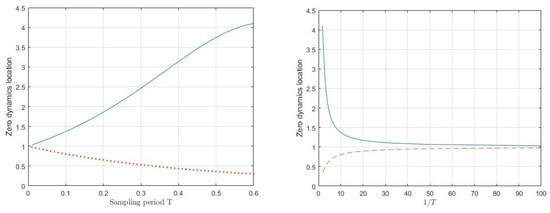
Figure 1. Zero dynamics location of sampled-data model for the Van der Pol system.

Next, we design a discrete-time model following a controller on the basis of the Van der Pol model with FROH and apply it to the original continuous-time Van der Pol system to further analyze the discrete dynamics behavior of the nonlinear Van der Pol system. It is obvious that the desired tracking objective of the output error results can be readily approached by being generated from the plant control input sequences in simulation (see Figure 2).

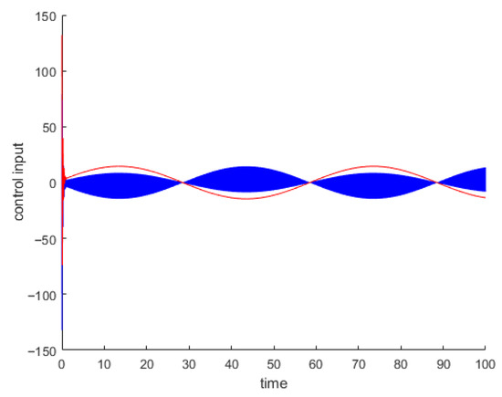
Figure 2. Control input of model following control for the Van der Pol system. The red and blue colors both indicate control input sequences.

In addition, we show the simulation results of the Van der Pol system with ε = 1, T = 0.01 in Figure 3. This paper considers the input into the original continuous Van der Pol system, through a fractional-order hold. We also give the output error of the Van der Pol system when the obtained discretization model and the true system output are used. Thus, good performance of the discrete dynamics behavior for the nonlinear Van der Pol controlled system can be achieved because the stability of the discrete zero dynamics of the nonlinear Van der Pol system are significantly improved in the manuscript, both in the theoretical results and simulation figures.

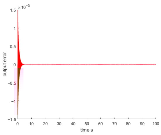
Figure 3. Error between the desired output and the true plant output for the Van der Pol system.

In this section, we focus on the (non)linear SISO system and study the discrete sampling model of the control plant under the FROH condition and delta operator, that is, the discrete sampling pulse function and the standard shape description for the discretization system. Moreover, the asymptotic characteristics of zero dynamics for a discrete sampling system are given, and the asymptotic expression of zero dynamics for a discrete-time system is given. Finally, the system identification based on sampled-data model output observations has been considered, and we also obtain the simulation results for the obtained sampled-data model.

5. Conclusions

In this paper, we focus on the adaptive (non)linear SISO system and study the discrete sampling model of the linear n-th order integrator system under FROH conditions, that is, the discrete sampling pulse function and the standard shape description of the discrete system. Furthermore, the asymptotic characteristics and stability of the zero dynamics of the nonlinear adaptive discrete sampling system are given, and an approximate expression of the discretization zero dynamics for the adaptive discrete system is given. Finally, these system identifications—which are based on nonlinear adaptive symmetry discrete sampling output observations—and the FROH discretization zero dynamics are compared. Additionally, the simulation results of the derived sampling model are obtained.

For future research, we can consider some of the following possible research topics: First, stochastic sampling zero dynamics have been considered by using the stochastic discrete-time or sampled-data plant. Second, we also consider the applications of nonlinear sampled-data models. In particular, our study examined the application of this model for nonlinear system identification. However, this is merely one example used to demonstrate the benefits of employing a sampled-data model, which is both simpler and more accurate than basic Euler integration. Finally, (non)linear continuous-time system identification with robustness can be discussed, and approximate incremental models that converge to the underlying true model will be developed. These alternative models allow for one to move seamlessly between continuous and discrete times.

References

- Åström, K.J.; Wittenmark, B. Adaptive Control, 3rd ed.; Courier Dover Publications: New York, NY, USA, 2008. [Google Scholar]
- Åström, K.J.; Wittenmark, B. Computer Controlled Systems, 3rd ed.; Courier Dover Publications: New York, NY, USA, 2011. [Google Scholar]
- Goodwin, G.C.; Aguero, J.C.; Garrido, M.E.; Salgado, M.E.; Yuz, J.I. Sampling and sampled-data models: The interface between the continuous world and digital algorithms. IEEE Control Syst. Mag. 2013, 33, 34–53. [Google Scholar]
- Yuz, J.I.; Goodwin, G.C. Sampled-Data Models for Linear and Nonlinear Systems; Springer: Berlin/Heidelberg, Germany, 2014. [Google Scholar]
- Ugalde, U.; Bárcena, R.; Basterretxea, K. Generalized sampled-data hold functions with asymptotic zero-order hold behavior and polynomic reconstruction. Automatica 2012, 48, 1171–1176. [Google Scholar] [CrossRef]
- Yuz, J.I.; Goodwin, G.C. On sampled-data models for nonlinear systems. IEEE Trans. Autom. Control. 2005, 50, 1477–1489. [Google Scholar] [CrossRef]
- Carrasco, D.S.; Goodwin, G.C. Vector measures of accuracy for sampled data models of nonlinear systems. IEEE Trans. Autom. Control. 2013, 58, 224–230. [Google Scholar] [CrossRef]
- Zeng, C.; Liang, S.; Li, H.; Su, Y. Discrete time systems with zero dynamics research present situation and the challenges of the future. Control. Theory Appl. 2013, 30, 1213–1230. (In Chinese) [Google Scholar]
- Åström, K.J.; Hagander, P.; Sternby, J. Zeros of sampled systems. Automatica 1984, 20, 31–38. [Google Scholar] [CrossRef]
- Ishitobi, M.; Nishi, M.; Kunimatsu, S. Asymptotic properties and stability criteria of zeros of sampled-data models for decouplable MIMO systems. IEEE Trans. Autom. Control 2013, 58, 2985–2990. [Google Scholar] [CrossRef]
- Zeng, C.; Liang, S.; Zhang, Y.; Zhong, J.; Su, Y. Improving the stability of discretization zeros with the Taylor method using a generalization of the fractional-order hold. Int. J. Appl. Math. Comput. Sci. 2014, 24, 745–757. [Google Scholar] [CrossRef]
- Carrasco, D.S.; Goodwin, G.C. Connecting filtering and control sensitivity functions. Automatica 2015, 50, 3319–3322. [Google Scholar] [CrossRef]
- Zeng, C.; Liang, S.; Zhong, J.; Su, Y. Improvement of the asymptotic properties of zero dynamics for sampled-data systems in the case of a time delay. Abstr. Appl. Anal. 2014, 2014, 1–12. [Google Scholar] [CrossRef]
- Weller, S.R.; Moran, W.; Ninness, B.; Pollington, A.D. Sampling zeros and the Euler-Fröbenius polynomials. IEEE Trans. Autom. Control. 2001, 46, 340–343. [Google Scholar] [CrossRef]
- Zhang, Y.; Kostyukova, O.; Chong, K.T. A new time-discretization for delay multiple-input nonlinear systems using the Taylor method and first order hold. Discret. Appl. Math. 2011, 159, 924–938. [Google Scholar] [CrossRef]
- Phillips, C.R.; Nagle, N.T. Digital control system analysis and design. IEEE Trans. Syst. Man Cybern. 1985, SMC-15, 452–453. [Google Scholar] [CrossRef]
- Passino, K.M.; Antsaklis, P.J. Inverse stable sampled low-pass systems. Int. J. Control. 1988, 47, 1905–1913. [Google Scholar] [CrossRef]
- Ishitobi, M. Stability of zeros of sampled system with fractional order hold. IEE Proc.-Control. Theory Appl. 1996, 143, 296–300. [Google Scholar] [CrossRef]
- Bàrcena, R.; de la Sen, M.; Sagastabeitia, I. Improving the stability properties of the zeros of sampled systems with fractional order hold. IEE Proc.-Control. Theory Appl. 2000, 147, 456–464. [Google Scholar] [CrossRef]
- Bàrcena, R.; de la Sen, M.; Sagastabeitia, I.; Collantes, J.M. Discrete control for a computer hard disk by using a fractional order hold device. IEE Proc.-Control. Theory Appl. 2001, 148, 117–124. [Google Scholar] [CrossRef]
- Bàrcena, R.; de la Sen, M. On the sufficiently small period for the convenient turning of fractional order hold circuits. IEE Proc.-Control. Theory Appl. 2003, 150, 183–188. [Google Scholar] [CrossRef]
- Bàrcena, R.; Etxebarria, A. Adaptive control of printing devices using fractional-order hold circuits adjusted through neural networks. J. Frankl. Inst. 2007, 344, 801–812. [Google Scholar] [CrossRef]
- Rubio, L.; De la Sen, M. Discrete-time model reference control schemes of milling forces using fractional order holds. In Proceedings of the 33rd Annual Conference of the IEEE Industrial Electronics Society, Taipei, Taiwan, 5–8 November 2007; pp. 798–803. [Google Scholar]
- Rubio, L.; De la Sen, M.; Longstaff, A.P.; Myers, A. Analysis of discrete time schemes for milling forces control under fractional order holds. Int. J. Precis. Manuf. 2013, 14, 735–744. [Google Scholar] [CrossRef][Green Version]
- Liang, S.; Ishitobi, M.; Zhu, Q. Improvement of stability of zeros in discrete-time multivariable system using fractional-order hold. Int. J. Control 2003, 76, 1699–1711. [Google Scholar] [CrossRef]
- Liang, S.; Ishitobi, M. The stability properties of the zeros of sampled models for time delay systems in fractional order hold case. Dyn. Contin. Discret. Impuls. Syst. Ser. B Appl. Algorithms 2004, 11, 299–312. [Google Scholar]
- Zeng, C.; Liang, S.; Li, H. Asymptotic properties of zero dynamics for nonlinear discretized systems with time delay via Taylor method. Nonlinear Dyn. 2015, 78, 11–25. [Google Scholar] [CrossRef]
- Ishitobi, M.; Nishi, M. Sampled-data models for nonlinear systems with a fractional-order hold. In Proceedings of the 18th IEEE International Conference on Control Applications Part of 2009 IEEE Multi-Conference on Systems and Control, Saint Petersburg, Russia, 8–10 July 2009; pp. 153–158. [Google Scholar]
- Nishi, M.; Ishitobi, M. Sampled-data models for affine nonlinear systems using a fractional-order hold and their zero dynamics. Artif. Life Robot. 2010, 15, 500–503. [Google Scholar] [CrossRef]
- Isidori, A. Nonlinear Control Systems: An Introduction; Springer: Berlin/Heidelberg, Germany, 1995. [Google Scholar]
- Isidori, A. The zero dynamics of a nonlinear system: From the origin to the latest progresses of a long successful story. Eur. J. Control. 2013, 19, 369–378. [Google Scholar] [CrossRef]
- Gillberg, J.; Ljung, L. Frequency-domain identification of continuous-time ARMA models from sampled data. Automatica 2010, 45, 1371–1378. [Google Scholar] [CrossRef]
- Chen, F.; Garnier, H. Frequency domain identification of continuous-time output-error models with time-delay from relay feedback tests. Automatica 2018, 98, 180–189. [Google Scholar] [CrossRef]
- Huang, C. A combined invariant-subspace and subspace identification method for continuous-time state–space models using slowly sampled multi-sine-wave data. Automatica 2022, 140, 1–10. [Google Scholar] [CrossRef]
- Yuz, J.I.; Goodwin, G.C. Robust Identification of Continuous-time Systems from Sampled Data. In Identification of Continuous-time Models from Sampled Data, Advances in Industrial Control; Garnier, H., Wang, L., Eds.; Springer: London, UK, 2008. [Google Scholar]
- Khalil, H. Nonlinear Systems, 3rd ed.; Prentice-Hall: Upper Saddle River, NJ, USA, 2002. [Google Scholar]
- Ishitobi, M.; Nishi, M.; Kunimatsu, S. Stability of zero dynamics of sampled-data nonlinear systems. In Proceedings of the 17th World Congress the International Federation of Automatic Control, Seoul, Republic of Korea, 6–11 July 2008; pp. 5969–5973. [Google Scholar]
- Ishitobi, M.; Nishi, M. Zero dynamics of Sampled-data models for nonlinear systems. In Proceedings of the 2008 American Control Conference, Westin Seattle Hotel, Seattle, Washington, DC, USA, 11–13 June 2009; pp. 1184–1189. [Google Scholar]
- Nishi, M.; Ishitobi, M. Sampled-data models and zero dynamics for nonlinear systems. In Proceedings of the ICROS-SICE International Joint Conference, Fukuoka International Congress Center, Fukuoka, Japan, 18–21 August 2009. [Google Scholar]
- Ojo, E.K.; Iyase, S.A.; Anake, T.A. Resonant fractional order differential equation with two dimensional kernel on the half-line. J. Math. Comput. Sci. 2024, 32, 122–136. [Google Scholar] [CrossRef]
- Luo, M.; Qiu, W.; Nikan, O.; Avazzadeh, Z. Second-order accurate, robust and efficient ADI Galerkin technique for the three dimensional nonlocal heat model arising in viscoelasticity. Appl. Math. Comput. 2023, 440, 1–21. [Google Scholar] [CrossRef]
Disclaimer/Publisher’s Note: The statements, opinions and data contained in all publications are solely those of the individual author(s) and contributor(s) and not of MDPI and/or the editor(s). MDPI and/or the editor(s) disclaim responsibility for any injury to people or property resulting from any ideas, methods, instructions or products referred to in the content. |
© 2025 by the authors. Licensee MDPI, Basel, Switzerland. This article is an open access article distributed under the terms and conditions of the Creative Commons Attribution (CC BY) license (https://creativecommons.org/licenses/by/4.0/).