Bayesian Inference on Stress–Strength Reliability with Geometric Distributions

Abstract

This paper investigates the estimation of the stress–strength reliability parameter $\rho =P(X\le Y)$, where stress (X) and strength $\left(Y\right)$ are independently modeled by geometric distributions. Objective Bayesian approaches are employed by developing Jeffreys, reference, and probability-matching priors for $\rho$, and their effects on the resulting Bayes estimates are examined. Posterior inference is carried out using the random-walk Metropolis–Hastings algorithm. The performance of the proposed Bayesian estimators is assessed through extensive Monte Carlo simulations based on average estimates, root mean squared errors, and frequentist coverage probabilities of the highest posterior density credible intervals. Furthermore, the applicability of the methodology is demonstrated using two real data sets.

1. Introduction

The estimation of stress–strength models has long been recognized as a fundamental topic in reliability theory. These models play an important role in various applied fields, particularly in engineering, quality assurance, and medical sciences. A significant portion of the statistical literature has focused on the estimation of the reliability parameter $\rho =P(X<Y)$, where X denotes the stress applied to a system, Y represents its strength, and $\rho$ quantifies the probability that the system can withstand the applied stress. It is worth emphasizing that numerous authors have investigated the estimation of the stress–strength reliability parameter $\rho$ using both frequentist and subjective Bayesian approaches across a range of continuous distributions and under various sampling schemes, and this topic continues to attract considerable attention in the statistical literature. For instance, Ref. [1] addressed this problem for the generalized exponential distribution; Ref. [2] studied it for the inverse Pareto distribution under progressively censored data; and Ref. [3] explored it for the exponential distribution based on generalized order statistics. In addition, Ref. [4] examined the Bayesian estimation of $\rho$ for the Lomax distribution under type-II hybrid censoring using an asymmetric loss function. On the other hand, several authors have employed objective Bayesian methods, for instance, Ref. [5] for the Weibull distribution, Ref. [6] for the generalized exponential stress–strength model, and Ref. [7] for the Fréchet stress–strength model. Related investigations based on discrete probability distributions include the works of [8] for Poisson data and [9] for the Poisson-geometric distribution. The geometric distribution has also been studied by [10,11,12] for complete data and for lower record data by [13]. However, in these latter studies, the Bayesian methods applied were subjective and limited in scope.

In this paper, we address the problem of estimating the stress–strength reliability parameter $\rho$ when both the stress X and the strength Y are modeled as independent geometric random variables with parameters ${\theta }_1$ and ${\theta }_2$, respectively. Accordingly, the reliability of the stress–strength system is given by

$$\rho =Pr(X\le Y)=\sum _{k=1}^{\infty }\sum _{j=k}^{\infty }{\theta }_1{\theta }_2{(1-{\theta }_1)}^{k-1}{(1-{\theta }_2)}^{j-1}={\displaystyle \frac{{\theta }_1}{1-(1-{\theta }_1)(1-{\theta }_2)}}.$$

(1)

The importance of studying stress–strength reliability under geometric distributions lies in its wide range of real-world applications, where reliable estimates with meaningful interpretation are required. For instance, in manufacturing quality control, let X denote the number of shocks a component tolerates before breaking and Y the number a stronger reference part withstands. The stress–strength reliability $\rho =Pr(X\le Y)$ then quantifies the probability that the component fails first. Since such failures typically occur after repeated shocks with a constant chance of breaking, the geometric distribution provides a natural model. A similar scenario arises in digital communication systems, where X represents the number of packet retransmissions until failure for a weaker channel and Y for a stronger channel. In this case, $\rho$ gives the probability that the weaker channel fails before the stronger one. Because packet transmissions follow repeated Bernoulli trials, the geometric distribution again offers a suitable framework. Finally, and more importantly, two additional real data examples highlighting the relevance of the stress–strength model are presented in the applications section.

Methods for estimating $\rho$ from discrete distributions have primarily relied on classical approaches, with the most common being the maximum likelihood (ML) estimator and subjective Bayesian methods, as clearly demonstrated in the works of [10,11,12]. While ML estimators have desirable properties, such as invariance and asymptotic efficiency, they are well known to exhibit bias, particularly with small sample sizes. Similar limitations arise when using subjective Bayesian methods, as these often involve multiple hyperparameters that must be elicited. However, the authors in the aforementioned papers employed the subjective Bayesian approach with hyperparameters that were subjectively chosen, rather than explicitly elicited, which can lead to potentially biased results. Specifically, the authors applied independent Beta priors to the parameters of the geometric distribution, i.e., ${\theta }_1\sim \mathrm{Beta}(a_1,b_1)$ and ${\theta }_2\sim \mathrm{Beta}(a_2,b_2)$, and arbitrarily selected the hyperparameters. One might ask why the subjective Bayesian approach did not involve a more rigorous elicitation of these parameters? The answer to this question lies in the criteria used for elicitation. For this case, four parameters need to be elicited, and there are numerous ways to do so, without a clear indication of which method will yield the most robust and reliable results. For example, one might set the mean and variance of the prior distributions, i.e., the considered beta distributions equal to the mean and variance of the geometric distribution. However, this approach can lead to infeasible solutions, such as negative values. Even if an alternative criterion is chosen and produces reasonable values, it still does not guarantee that the method will be applicable in all cases or lead to reliable results. Certainly, the most appealing approach would be to leverage prior information (past knowledge) about the parameters ${\theta }_1$ and ${\theta }_2$. Unfortunately, such prior information is often unavailable in many situations. Furthermore, the authors did not train their methods on real data, which limits the generalizability and robustness of their results.

Alternatively, we adopt a Bayesian approach for estimating $\rho$ using non-informative priors. Our motivation for using such priors, in addition to the importance of studying $\rho$ under geometric distributions, lies in its wide range of real-world applications. The reasons for choosing this approach are as follows: (i) this is the first study to consider objective Bayesian inference for $\rho$; (ii) the priors considered in this study are informative yet contain minimal information; (iii) the priors eliminate the need for hyperparameter elicitation; (iv) the priors are obtained using formal rules; and (v) the priors possess the flavor of invariance, or certain modifications that offer improved performance, particularly in high-dimensional parameter settings, or alternative priors capable of producing credible intervals with coverage properties comparable to those of frequentist confidence intervals.

Before proceeding, we would like to point out that $\rho$ is a function of the model parameters. In such cases, constructing non-informative priors requires particular care, except for Jeffreys’ prior, which is invariant by design. Other types of priors, such as matching and reference priors, are generally not invariant under reparameterization. For instance, suppose matching priors are developed under the assumption that ${\theta }_1$ is the parameter of interest and ${\theta }_2$ is a nuisance parameter, or vice versa. If a one-to-one transformation is then applied to express the model in terms of $\rho$, the resulting prior is not guaranteed to be a matching prior for $\rho$. This is because the inverse transformation yields reference or matching priors that are valid for ${\theta }_1$ and ${\theta }_2$, depending on which parameter was treated as influential, but not necessarily for a derived parameter like $\rho$. A similar issue arises with reference priors. While it might be argued, as shown by [14], that reference and matching priors are invariant, this invariance only holds when such priors are developed directly for $\rho$ as a function of ${\theta }_1$ and ${\theta }_2$, followed by an appropriate transformation. In that case, the resulting priors retain their desired properties with respect to $\rho$. A comparable situation is discussed in [15], who provided Bayesian inference for the entropy of the Lomax distribution, a quantity that also depends on the model parameters, and demonstrated that the reference and matching priors for this entropy cannot be derived from those of the model parameters. For further developments and illustrative examples, the reader is referred to [14], who specifically constructed matching priors for functions of model parameters.

The rest of the paper is organized as follows. Likelihood-based inference for $\rho$ is presented in Section 2. In Section 3, we derive non-informative priors for $\rho$, including Jeffreys, reference, and probability-matching priors. Section 4 reports a simulation study conducted via MCMC to assess the performance of the Bayes estimators of $\rho$ under various objective priors. In this section, we also provide the average estimates, standard errors, and coverage probabilities of the 95% credible intervals. The compatibility of the proposed priors is further examined in Section 5 using the posterior predictive distribution. In Section 6, the practical utility of the stress–strength reliability measure for the geometric distribution is demonstrated through two real data applications. Finally, concluding remarks are given in Section 7.

2. Likelihood-Based Inference for $\mathit{\rho }$

Let $\mathbf{X}={(X_1,\dots ,X_n)}^t$ and $\mathbf{Y}={(Y_1,\dots ,Y_m)}^t$ be independent random samples from $\mathrm{GE}\left({\theta }_1\right)$ and $\mathrm{GE}\left({\theta }_2\right),$ respectively, where GE(.) denotes the geometric distribution. Then, the likelihood function of $({\theta }_1,{\theta }_2)$ based on the realizations $\mathbf{x}={(x_1,\dots ,x_n)}^t$ and $\mathbf{y}={(y_1,\dots ,y_m)}^t,$ is

$$\begin{array}{cc}\hfill L({\theta }_1,{\theta }_2|\mathbf{x},\mathbf{y})& =\prod _{i=1}^n\left\{{\theta }_1{(1-{\theta }_1)}^{x_i-1}\right\}\prod _{j=1}^m\left\{{\theta }_2{(1-{\theta }_2)}^{y_j-1}\right\},\hfill \\ \hfill & ={\theta }_1^n{\theta }_2^m{\left(1-{\theta }_1\right)}^{T_1-n}{\left(1-{\theta }_2\right)}^{T_2-m},(n,m)\in \mathbb{N}\times \mathbb{N},\hfill \end{array}$$

(2)

where $T_1={\sum }_{i=1}^n{X}_i$ and $T_2={\sum }_{j=1}^m{Y}_j.$ The ML estimates of $({\theta }_1,{\theta }_2)$ can be obtained by maximizing the log-likelihood function with a mathematical form given by

$$\begin{array}{c}\hfill \ell ({\theta }_1,{\theta }_2)=nln\left({\theta }_1\right)+mln\left({\theta }_2\right)+(T_1-n)ln(1-{\theta }_1)+(T_2-m)ln(1-{\theta }_1).\end{array}$$

The partial derivatives of $\ell ({\theta }_1,{\theta }_2)$ with ${\theta }_1$ and ${\theta }_2$ are given below:

$$\begin{array}{c}\hfill {\displaystyle \frac{\partial \ell ({\theta }_1,{\theta }_2)}{\partial {\theta }_1}}={\displaystyle \frac{n}{{\theta }_1}}-{\displaystyle \frac{T_1-n}{1-{\theta }_1}}\mathrm{and}{\displaystyle \frac{\partial \ell ({\theta }_1,{\theta }_2)}{\partial {\theta }_2}}={\displaystyle \frac{m}{{\theta }_2}}-{\displaystyle \frac{T_2-m}{1-{\theta }_2}}.\end{array}$$

On solving the above equations, the ML estimates of $({\theta }_1,{\theta }_2)$ are given by ${\widehat{\theta }}_1={\displaystyle \frac{n}{T_1}}$ and ${\widehat{\theta }}_2={\displaystyle \frac{m}{T_2}}$. Since $E\left(X\right)={\displaystyle \frac{1}{{\theta }_1}}$ and $E\left(Y\right)={\displaystyle \frac{1}{{\theta }_2}}$, the elements of the Fisher information matrix are computed via

$$-\mathbb{E}\left({\displaystyle \frac{{\partial }^2\ell ({\theta }_1,{\theta }_2)}{\partial {\theta }_1^2}}\right)=\left({\displaystyle \frac{n}{{\theta }_1^2}}+{\displaystyle \frac{\mathbb{E}(T_1-n)}{{(1-{\theta }_1)}^2}}={\displaystyle \frac{n}{{\theta }_1^2(1-{\theta }_1)}}\right),$$

$$\mathbb{E}\left({\displaystyle \frac{{\partial }^2\ell ({\theta }_1,{\theta }_2)}{\partial {\theta }_1\partial {\theta }_1}}\right)=\mathbb{E}\left({\displaystyle \frac{{\partial }^2\ell ({\theta }_1,{\theta }_2)}{\partial {\theta }_2\partial {\theta }_1}}\right)=0,$$

and

$$-\mathbb{E}\left({\displaystyle \frac{{\partial }^2\ell ({\theta }_1,{\theta }_2)}{\partial {\theta }_2^2}}\right)={\displaystyle \frac{m}{{{\theta }_2}^2}}+{\displaystyle \frac{\mathbb{E}(T_2-m)}{{(1-{\theta }_2)}^2}}={\displaystyle \frac{m}{{{\theta }_2}^2(1-{\theta }_2)}}.$$

Therefore, we have that

$$\begin{array}{c}\hfill \mathbf{F}({\theta }_1,{\theta }_2)=\left(\begin{array}{cc}-\mathbb{E}({\displaystyle \frac{{\partial }^2\ell ({\theta }_1,{\theta }_2)}{\partial {\theta }_1^2}}& -\mathbb{E}\left({\displaystyle \frac{{\partial }^2\ell ({\theta }_1,{\theta }_2)}{\partial {\theta }_1\partial {\theta }_1}}\right)\\ -\mathbb{E}\left({\displaystyle \frac{{\partial }^2\ell ({\theta }_1,{\theta }_2)}{\partial {\theta }_2\partial {\theta }_1}}\right)& -\mathbb{E}\left({\displaystyle \frac{{\partial }^2\ell ({\theta }_1,{\theta }_2)}{\partial {\theta }_2^2}}\right)\end{array}\right)=\left(\begin{array}{cc}{\displaystyle \frac{n}{{\theta }_1^2(1-{\theta }_1)}}& 0\\ 0& {\displaystyle \frac{m}{{\theta }_2^2(1-{\theta }_2)}}\end{array}\right),\end{array}$$

(3)

The following results are required to establish the asymptotic normality of the ML estimate of $\rho$.

Lemma 1.

The ML estimates ${\widehat{\theta }}_1={\displaystyle \frac{n}{T_1}}$ and ${\widehat{\theta }}_2={\displaystyle \frac{m}{T_2}}$ are consistent estimators of ${\theta }_1$ and ${\theta }_2$, respectively.

Proof. 

We provide only the proof of the consistency of ${\widehat{\theta }}_1={\displaystyle \frac{n}{T_1}}$ for ${\theta }_1$, and the proof for the other estimator can be handled similarly. Since $W_n:={\displaystyle \frac{T_1}{n}}={\displaystyle \frac{{\sum }_{i=1}^n{X}_i}{n}}$, it follows from the strong law of large numbers that ${\displaystyle \frac{T_1}{n}}$ converges in probability to $\mathbb{E}\left(X_1\right)={\displaystyle \frac{1}{{\theta }_1}}$. Now, since $g\left(x\right)={\displaystyle \frac{1}{x}}$ for $x>0$ is a continuous function, it follows that $g\left(W_n\right)={\displaystyle \frac{n}{T_1}}$ converges to $g\left(\mathbb{E}\left(X_1\right)\right)={\theta }_1$.    □

The following theorem establishes that the ML estimates of ${\theta }_1$ and ${\theta }_2$ are asymptotically bivariate normal. The conditions required for this are as follows: The likelihood function must be identifiable and differentiable, and the true parameter value must lie in the interior of the parameter space. The partial derivatives of the log-likelihood function must be continuous and have a unique solution at the true parameter. Additionally, the observed Fisher information must converge to its expected value as the sample size increases, and the Fisher information matrix must be finite and positive definite. Finally, the log-likelihood function should satisfy smoothness conditions. For more information on these regularity conditions and the establishment of the asymptotic normality of the MLE, see [16] (1993, p. 132).

Theorem 1.

We have that, as $n\to \infty ,$ $m\to \infty ,$ and ${\displaystyle \frac{n}{m}}\to p,$ ${\left(\sqrt{n}({\widehat{\theta }}_1-{\theta }_1),\sqrt{m}({\widehat{\theta }}_2-{\theta }_2)\right)}^t\Rightarrow {\mathrm{N}}_2(0,{\mathbf{H}}^{-1}({\theta }_1,{\theta }_2)),$ where ⇒ stand for convergence in distribution, and ${\mathrm{N}}_2(.,.)$ stand for bivariate normal distribution, and

$$\begin{array}{c}\hfill \mathbf{H}({\theta }_1,{\theta }_2))=\left(\begin{array}{cc}{\displaystyle \frac{1}{{\theta }_1^2(1-{\theta }_1)}}& 0\\ 0& {\displaystyle \frac{p}{{\theta }_2^2(1-{\theta }_2)}}\end{array}\right),\end{array}$$

(4)

Proof. 

Thanks to the exponential family of distributions, which satisfies all the mentioned regularity conditions, asymptotic normality follows. Since the geometric distribution belongs to the exponential family, the asymptotic normality of its MLEs is guaranteed. The above matrix is obtained by virtue of the regularity condition given in the preceding paragraph, which states that the average observed Fisher information must converge to its expected value as the sample size increases. To see this, the average observed Fisher information matrix, after simple rearrangement, is

$${\displaystyle \frac{1}{n}}\mathbf{J}({\theta }_1,{\theta }_2)=\left(\begin{array}{cc}{\displaystyle \frac{1}{{\theta }_1^2}}+{\displaystyle \frac{\overline{X}-1}{{(1-{\theta }_1)}^2}}& 0\\ 0& {\displaystyle \frac{m}{n}}\left({\displaystyle \frac{1}{{\theta }_2^2}}+{\displaystyle \frac{\overline{Y}-1}{{(1-{\theta }_2)}^2}}\right)\end{array}\right),$$

Since $\overline{X}$ and $\overline{Y}$ converges in probability to $1/{\theta }_1$ and $1/{\theta }_2$ in probability as $n,m\to \infty$ respectively and by mean of the assumption that $m/n\to p\in (0,1],$ it follows that ${\displaystyle \frac{1}{n}}\mathbf{J}({\theta }_1,{\theta }_2)$ converges in probability to $\mathbf{H}({\theta }_1,{\theta }_2)).$ Noticed that when $p=1$ implies $m=n$ and hence $\mathbf{H}({\theta }_1,{\theta }_2)$ is the Fisher information matrix of independent geometric distributions per unit of observation, and this completes the proof.    □

Theorem 2

([16] (1993, p. 132)). Suppose that $\sqrt{n}(W_n-\mathit{\theta })\Rightarrow {\mathrm{N}}_k(\mathbf{0},\mathbf{\Sigma }),$ were $W_n$ is k-dimensional random vectors, $\mathit{\theta }={({\theta }_1,\dots ,{\theta }_k)}^t,$ and Σ is the variance-covariance matrix. Let $g:{\mathbb{R}}^k\to \mathbb{R}$ be a real-valued function with $\nabla :=(\partial g\left(\mathit{\theta }\right)/\partial {\theta }_1,\dots ,\partial g\left(\mathit{\theta }\right)/\partial {\theta }_k)\ne \mathbf{0}$ and continuous in a neighborhood of $\mathit{\theta }.$ Then, $\sqrt{n}(g\left(W_n\right)-g\left(\mathit{\theta }\right))\Rightarrow {\mathrm{N}}_k(\mathbf{0},{\nabla }^t\mathbf{\Sigma }\nabla ).$

The above theorem is usually referred to as the Delta method. Here, we establish the first results relating to the estimate of $\rho$.

Theorem 3.

As $n\to \infty ,$ $m\to \infty ,$ and ${\displaystyle \frac{n}{m}}\to p,$ we have $\sqrt{n}(\widehat{\rho }-\rho )\Rightarrow \mathrm{N}(0,{\sigma }_{\rho }^2),$ where

$${\sigma }_{\rho }^2={\displaystyle \frac{{\theta }_1^2{\theta }_2^2(1-{\theta }_1)}{{\delta }^2}}\left\{1+p(1-{\theta }_1)(1-{\theta }_2)\right\},$$

and $\delta ={\left\{1-(1-{\theta }_1)(1-{\theta }_2)\right\}}^2.$

Proof. 

We have from, Theorem 1 that as $n\to \infty ,$ $m\to \infty ,$${\left(\sqrt{n}({\widehat{\theta }}_1-{\theta }_1),\sqrt{m}({\widehat{\theta }}_2-{\theta }_2)\right)}^t\Rightarrow {\mathrm{N}}_2(0,{\mathbf{H}}^{-1}({\theta }_1,{\theta }_2)),$ where $\mathbf{H}({\theta }_1,{\theta }_2)$ is given in (4). Clearly, $\rho :(0,1)\times (0,1)\to (0,1),$ where

$$\rho =:\rho ({\theta }_1,{\theta }_2)={\displaystyle \frac{{\theta }_1}{1-(1-{\theta }_1)(1-{\theta }_2)}}.$$

Notice that the $\rho$ plays the role as the $g(.)$ function in Theorem 2, and hence we have that as $n\to \infty ,$ $m\to \infty ,$ and ${\displaystyle \frac{n}{m}}\to p,$ $\sqrt{n}(\widehat{\rho }-\rho )\Rightarrow \mathrm{N}(0,{\sigma }_{\rho }^2),$ where

$$\begin{array}{c}\hfill {\sigma }_{\rho }^2={\nabla }^t{\mathbf{H}}^{-1}({\theta }_1,{\theta }_2)\nabla ,\end{array}$$

(5)

and

$$\nabla ={\left({\displaystyle \frac{\partial \rho }{\partial {\theta }_1}},{\displaystyle \frac{\partial \rho }{\partial {\theta }_2}}\right)}^t={\left({\displaystyle \frac{{\theta }_2}{{\left\{1-(1-{\theta }_1)(1-{\theta }_2)\right\}}^2}},-{\displaystyle \frac{{\theta }_1(1-{\theta }_1)}{{\left\{1-(1-{\theta }_1)(1-{\theta }_2)\right\}}^2}}\right)}^t.$$

In view of (5), we have that

$${\sigma }_{\rho }^2={\displaystyle \frac{{\theta }_1^2{\theta }_2^2(1-{\theta }_1)}{{\delta }^2}}\left\{1+p(1-{\theta }_1)(1-{\theta }_2)\right\},$$

as desired.    □

Since ${\widehat{\theta }}_1$ and ${\widehat{\theta }}_2$ are consistence estimators by the mean of Lemma 1 an approximate $(1-\alpha )100\%$ confidence interval of $\rho$ is

$$\widehat{\rho }\pm z_{{\displaystyle \frac{\alpha }{2}}}{\widehat{\sigma }}_{\rho },\mathrm{where}{\widehat{\sigma }}_{\rho }^2={\displaystyle \frac{{\widehat{\theta }}_1^2{\widehat{\theta }}_2^2(1-{\widehat{\theta }}_1)}{{\widehat{\delta }}^2}}\left\{1+p(1-{\widehat{\theta }}_1)(1-{\widehat{\theta }}_2)\right\}.$$

3. Bayes Inferences: Objective Priors

In this section, we construct several important objective (non-informative) priors for the parameter $\rho$, including the Jeffreys prior, reference priors, and probability matching priors. These priors are developed to ensure minimal informativeness while retaining desirable inferential properties. Following the construction of each prior, we examine the propriety and finiteness of the resulting posterior distributions. We then proceed to derive the Bayes estimates of $\rho$ under the squared error loss (SEL). To facilitate the construction of certain priors, particularly the reference and matching priors, we reparameterize the original model in terms of the parameter $\rho$. While the Jeffreys prior is invariant under one-to-one transformations and thus can be obtained directly without reparameterization, such transformations are crucial for deriving the reference and matching priors, as they depend explicitly on the parameter of interest. Therefore, we consider a one-to-one transformation from

$${\Omega }_{({\theta }_1,{\theta }_2)}=\{({\theta }_1,{\theta }_2):0<{\theta }_1<1,0<{\theta }_2<1\}\mathrm{onto}{\Omega }_{(\rho ,\omega )}=\{(\rho ,\omega ):0<\rho <1,0<\omega <1\},$$

where

$$\begin{array}{c}\hfill \rho ={\displaystyle \frac{{\theta }_1}{1-(1-{\theta }_1)(1-{\theta }_2)}}\mathrm{and}\omega ={\theta }_2,\end{array}$$

(6)

along with the inverse of the transformation,

$${\theta }_1={\displaystyle \frac{\rho \omega }{1-(1-\omega )\rho }}\mathrm{and}{\theta }_2=\omega .$$

Therefore, the likelihood function of $(\rho ,\omega )$ based on ${(\mathbf{x},\mathbf{y})}^t$ is

$$\begin{array}{cc}\hfill \mathbb{L}(\rho ,\omega |\mathbf{x},\mathbf{y})& \propto {\rho }^n{\omega }^{n+m}{(1-\rho )}^{T_1-n}{(1-\omega )}^{T_2-m}{\left(1-\rho (1-\omega )\right)}^{-T_1}.\hfill \end{array}$$

(7)

We now aim to obtain the Fisher information matrix corresponding to the parameters $\rho$ and $\omega$. To this end, we first evaluate the Jacobian matrix of the transformation $\mathbf{M}={\displaystyle \frac{\partial ({\theta }_1,{\theta }_2)}{\partial (\rho ,\omega )}}$ which is given by

$$\begin{array}{c}\hfill \mathbf{M}=\left(\begin{array}{cc}{\displaystyle \frac{\omega }{{(1-(1-\omega )\rho )}^2}}& {\displaystyle \frac{\rho (1-\rho )}{{(1-(1-\omega )\rho )}^2}}\\ & \\ 0& 1\end{array}\right).\end{array}$$

(8)

Using Equations (3) and (8), the Fisher information matrix for the parameters $\rho$ and $\omega ,$ denoted by $\Sigma (\rho ,\omega )$, is obtained through the relation $\Sigma (\rho ,\omega )={\mathbf{M}}^T\mathbf{F}\mathbf{M}.$ This result is summarized in the following lemma.

Theorem 4.

The Fisher information matrix of $(\rho ,\omega )$ has the following form

$$\Sigma (\rho ,\omega )=\left(\begin{array}{cc}{\sigma }_{\rho \rho }& {\sigma }_{\rho \omega }\\ & \\ {\sigma }_{\omega \rho }& {\sigma }_{\omega \omega }\end{array}\right)=\left(\begin{array}{cc}{\displaystyle \frac{n}{{\rho }^2(1-\rho )(1-(1-\omega )\rho )}}& {\displaystyle \frac{n}{\rho \omega (1-(1-\omega \left)\rho \right)}}\\ & \\ {\displaystyle \frac{n}{\rho \omega (1-(1-\omega \left)\rho \right)}}& {\displaystyle \frac{m\omega +(n+m)(1-\omega )(1-\rho )}{{\omega }^2(1-\omega )(1-(1-\omega )\rho )}}\end{array}\right).$$

(9)

3.1. Jeffreys Prior

The first non-informative prior we consider is the Jeffreys prior, which is commonly used in Bayesian inference due to its simple derivation from the Fisher information matrix and its invariance property. In general, this type of prior is improper, as are many other non-informative priors. Additionally, it may be inappropriate when the dimensionality of the model increases. Therefore, from Equation (9), the Jeffreys prior of $(\rho ,\omega )$ is

$${\pi }_J(\rho ,\omega )\propto {\displaystyle \frac{1}{\rho \omega {\left\{(1-\rho )(1-\omega )(1-(1-\omega \left)\rho \right)\right\}}^{1/2}}},0<\rho <1,0<\omega <1.$$

(10)

The joint posterior of $(\rho ,\omega )$ under ${\pi }_J(\rho ,\omega )$ in (10) is

$${\pi }_J(\rho ,\omega |\mathbf{x},\mathbf{y})\propto {\rho }^{n-1}{\omega }^{n+m-1}{(1-\rho )}^{T_1-n-1/2}{(1-\omega )}^{T_2-m-1/2}{\left(1-\rho (1-\omega )\right)}^{-T_1-1/2}.$$

(11)

Theorem 5.

The posterior ${\pi }_J(\rho ,\omega |\mathbf{x},\mathbf{y})$ is proper if and only if $m>2,$ $T_1>n-1/2$ and $T_2>m-1/2.$

Proof. 

We have that for sufficiently small values $(\rho ,\omega )\to (0,0),$ we have that ${\pi }_J(\rho ,\omega |\mathbf{x},\mathbf{y})\sim {\rho }^{n-1}{\omega }^{n+m-1},$ and hence ${\int }_0^1{\int }_0^1{\pi }_J(\rho ,\omega |\mathbf{x},\mathbf{y})d\omega d\rho =1/\left(n\right(n+m\left)\right)<+\infty .$ Similarly, for the values $(\rho ,\omega )\to (1,1)$, we have that ${\pi }_J(\rho ,\omega |\mathbf{x},\mathbf{y})\sim {(1-\rho )}^{T_1-n-1/2}{(1-\omega )}^{T_2-m-1/2}.$ So, we have that

$$\begin{array}{cc}\hfill {\int }_0^1{\int }_0^1{\pi }_J(\rho ,\omega |\mathbf{x},\mathbf{y})d\omega d\rho & ={\int }_0^1{\int }_0^1{(1-\rho )}^{T_1-n-1/2}{(1-\omega )}^{T_2-m-1/2}d\omega d\rho \hfill \\ \hfill & ={\displaystyle \frac{1}{(T_1-n+1/2)(T_2-m+1/2)}}.\hfill \end{array}$$

Thus, the expression is finite and positive if and only if $T_1>n-1/2$ and $T_2>m-1/2$. Next, when the values of $(\rho ,\omega )$ are close to the singularity, i.e., $(\rho ,\omega )\to (1,0)$, we consider the first-order Taylor expansion of $g(\rho ,\omega ):=1-\rho (1-\omega )$ around $(1,0)$. We then obtain $1-\rho (1-\omega )\approx 1-\rho +\omega ,$ and it follows that

$$\begin{array}{cc}\hfill {\int }_0^1{\int }_0^1{\pi }_J(\rho ,\omega \mid \mathbf{x},\mathbf{y})d\omega d\rho & \propto {\int }_0^1{\int }_0^1{\omega }^{n+m-1}{(1-\rho )}^{T_1-n-\frac{1}{2}}{(1-\rho +\omega )}^{-T_1-\frac{1}{2}}d\omega d\rho \hfill \\ \hfill & ={\int }_0^1{\int }_0^1{u}^{n+m-1}{v}^{T_1-n-\frac{1}{2}}{(v+u)}^{-T_1-\frac{1}{2}}dudv,\hfill \end{array}$$

(12)

where in the last equation we used the transformation $u=\omega$ and $v=1-\rho .$ Now, to check the finitess of the above double integral, we consider the transformation $u=ts$ and $v=t(1-s)$ with Jacobian of transformation $\left|J\right|=t^{-1},$

$$\begin{array}{cc}\hfill {\int }_0^1{\int }_0^1{\displaystyle \frac{u^{n+m-1}{v}^{T_1-n-1/2}}{{\left(v+u\right)}^{T_1+1/2}}}dudv& ={\int }_0^1{\int }_0^1{t}^{m-3}{s}^{n+m-1}{(1-s)}^{T_1-n-1/2}dsdt,\hfill \\ \hfill & ={\displaystyle \frac{\Gamma (n+m)\Gamma (T_1-n+1/2)}{(m-2)\Gamma (T_1+m+1/2)}}.\hfill \end{array}$$

Hence, the right-hand side of the above equation is finite and positive, provided that $m>2$.    □

3.2. Approximate Reference Priors

The reference prior, originally introduced by [17] and further refined in the same work, serves as an enhancement of Jeffreys’ prior, particularly in multi-parameter settings where Jeffreys’ prior may not perform well; see [18]. A key feature of this approach is the partitioning of model parameters into groups based on their inferential priority. The derivation of the reference prior follows a general algorithm outlined in [17]. Notably, one significant result arising from this algorithm, which proves useful in various applications, is that it avoids the need for nested compact subsets in the nuisance parameter space. This is formally presented in the following proposition.

Proposition 1

([19] (2000, p. 328)). Let ψ be the parameter of interest and suppose that λ is the nuisance parameter. Let

$$D_{\psi }(\psi ,\lambda ):={\displaystyle \frac{det\left(\mathbf{I}(\psi ,\lambda )\right)}{I_{\lambda \lambda }(\psi ,\lambda )}},$$

where $\mathbf{I}(\psi ,\lambda )$ is the Fisher information matrix and $I_{\lambda \lambda }(\psi ,\lambda )$ is the bottom-right element of $I(\psi ,\lambda ).$ If the parameter of interest ψ is independent of the nuisance parameter space $\Lambda \left(\psi \right),$ and if

$$D_{\psi }^{{\displaystyle \frac{1}{2}}}(\psi ,\lambda )=h_1\left(\psi \right)g_1\left(\lambda \right)\mathit{and}{I}_{\lambda \lambda }^{{\displaystyle \frac{1}{2}}}(\psi ,\lambda )=h_2\left(\psi \right)g_2\left(\lambda \right),$$

then the reference prior with respect to the ordered group $(\psi ,\lambda )$ is

$$\pi (\psi ,\lambda )=h_1\left(\psi \right)g_2\left(\lambda \right).$$

It is worth emphasizing that neither the procedure outlined in [17] nor the result in Proposition 1 yields an explicit form of the reference prior for $\rho$. As an alternative, we construct an approximate reference prior by leveraging the result in Proposition 1.

Proposition 2.

The approximate reference prior for the ordered group parameters $(\rho ,\omega )$ is

(i)

for sufficiently small $\rho ,$

$$\begin{array}{c}\hfill {\pi }_{R_1}(\rho ,\omega )\propto {\displaystyle \frac{\sqrt{m\omega +(n+m)(1-\omega )}}{\rho \omega {(1-\omega )}^{1/2}}},0<\rho <1,0<\omega <1.\end{array}$$

(13)

(ii)

for $\rho \to 1,$ we have that

$$\begin{array}{c}\hfill {\pi }_{R_2}(\rho ,\omega )\propto {\displaystyle \frac{1}{\sqrt{\omega (1-\rho )(1-\omega )}}},0<\rho <1,0<\omega <1.\end{array}$$

(14)

Proof. 

We provide the proof only for part (i). We have that

$$\begin{array}{cc}\hfill D_{\rho }^{{\displaystyle \frac{1}{2}}}(\rho ,\omega )& ={\displaystyle \frac{1}{\rho {(1-\rho )}^{1/2}{\left\{m\omega +(n+m)(1-\omega )(1-\rho )\right\}}^{1/2}}},\hfill \\ \hfill & \sim {\displaystyle \frac{1}{\rho {\left\{m\omega +(n+m)(1-\omega )\right\}}^{1/2}}},\mathrm{as}\rho \to 0\hfill \\ \hfill & :=h_1\left(\rho \right)g_1\left(\omega \right)\hfill \end{array}$$

where $h_1\left(\rho \right)={\rho }^{-1}$ and $g_1\left(\omega \right)=\left[m\omega +(n+m)(1-\omega )\right\}{]}^{-1/2}.$ Now

$$\begin{array}{cc}\hfill {\sigma }_{\omega \omega }^{{\displaystyle \frac{1}{2}}}(\rho ,\omega )& \sim {\displaystyle \frac{m\omega +(n+m)(1-\omega )}{{\omega }^2(1-\omega )}},\mathrm{as}\rho \to 0\hfill \\ \hfill & :=h_2\left(\rho \right)g_2\left(\omega \right),\hfill \end{array}$$

where $h_2\left(\rho \right)=1$ and $g_2\left(\omega \right)={\sigma }_{\omega \omega }^{{\displaystyle \frac{1}{2}}}(\rho ,\omega ).$ In view of Proposition 1, it follows that the approximate reference prior for the ordered group $(\rho ,\omega )$ is the one given in (13).    □

Theorem 6.

Under the assumption of Theorem 5, the posterior distributions under ${\pi }_{R_1}(\rho ,\omega |\mathbf{x},\mathbf{y})$ and ${\pi }_{R_2}(\rho ,\omega |\mathbf{x},\mathbf{y})$ are proper distributions.

Proof. 

We provide the proof for ${\pi }_{R_1}(\rho ,\omega |\mathbf{x},\mathbf{y}).$ The proof of ${\pi }_{R_2}(\rho ,\omega |\mathbf{x},\mathbf{y})$ is quite similar to the proof in Theorem. Since ${(m\omega +(n+m)(1-\omega ))}^{1/2}$ is a decreasing function in $\omega ,$ we have

$${\pi }_{R_1}(\rho ,\omega )\le {\displaystyle \frac{\sqrt{n+m}}{\rho \omega {(1-\omega )}^{1/2}}}.$$

Therefore, we have that

$${\pi }_{R_1}(\rho ,\omega |\mathbf{x},\mathbf{y})\le K{\rho }^{n-1}{\omega }^{n+m-1}{(1-\rho )}^{T_1-n}{(1-\omega )}^{T_2-m-1/2}{\left(1-\rho (1-\omega )\right)}^{-T_1},$$

where $K=\sqrt{n+m}.$ Similar to the proof in Theorem 5, we have for sufficiently small values of $\rho$ and $\omega$ that ${\pi }_{R_1}(\rho ,\omega |\mathbf{x},\mathbf{y})\le K{\rho }^{n-1}{\omega }^{n+m-1}$ it then follows that the posterior distribution is finite, i.e., ${\int }_0^1{\int }_0^1{\pi }_{R_1}(\rho ,\omega |\mathbf{x},\mathbf{y})d\omega d\rho \le K{\int }_0^1{\int }_0^1{\pi }_{R_1}{\rho }^{n-1}{\omega }^{n+m-1}\le d\omega d\rho \le K/(n(n+m)<+\infty .$ When $\rho$ and $\omega$ are close to $1,$ it then follows for $T_1>n-1$ and $T_2>m-1/2$ that ${\int }_0^1{\int }_0^1{\pi }_{R_1}(\rho ,\omega |\mathbf{x},\mathbf{y})d\omega d\rho \le K{\int }_0^1{\int }_0^1{(1-\rho )}^{T_1-n}{(1-\omega )}^{T_2-m-1/2}d\omega d\rho <+\infty .$ Finally, when the values of $(\rho ,\omega )$ close to $(\rho ,\omega )\to (1,0),$ the first-order Taylor expansion for $g(\rho ,\omega ):=(1-\rho (1-\omega \left)\right)$ around $(1,0),$ implies that $1-\rho (1-\omega )\approx 1-\rho +\omega ,$ it then follows that

$${\pi }_{R_1}(\rho ,\omega |\mathbf{x},\mathbf{y})\le K{\omega }^{n+m-1}{(1-\rho )}^{T_1-n-1/2}{\left(1-\rho +\omega \right)}^{-T_1-1/2}.$$

Therefore, we have that

$${\int }_0^1{\int }_0^1{\pi }_{R_1}(\rho ,\omega |\mathbf{x},\mathbf{y})d\omega d\rho \le K{\int }_0^1{\int }_0^1{\omega }^{n+m-1}{(1-\rho )}^{T_1-n-1/2}{\left(1-\rho +\omega \right)}^{-T_1}d\omega d\rho .$$

Similarly to the analysis of (12), the above integral is finite.    □

3.3. Probability Matching Prior

Probability matching priors for the parameter of interest were introduced by [20] to ensure that the posterior probabilities of specified intervals exactly or approximately match their corresponding frequentist coverage probabilities. Mathematically speaking, let be $\pi (\rho ,\omega )$ be a given prior of $(\rho ,\omega )$ with parameter of interest $\rho$ and $\omega$ is the nuisance parameter and ${\rho }^{(1-\alpha )}(\pi ,\mathbf{X},\mathbf{Y})$ is the $(1-\alpha )$th percentile of the marginal posterior distribution of $\rho$, where $\mathbf{X}=(X_1,X_2,\dots ,X_n)$ and $\mathbf{Y}=(Y_1,Y_2,\dots ,Y_m)$ are the sample data. Then, $\pi (·)$ is called a second-order probability matching prior if

$$\begin{array}{c}\hfill Pr\left(\rho \le {\rho }^{(1-\alpha )}(\pi ,\mathbf{X},\mathbf{Y})\right)=1-\alpha +o\left(n^{-1}\right),\end{array}$$

holds for all $\alpha \in (0,1).$ It is worth emphasizing that Jeffreys prior achieves probability matching with an asymptotic error of order $n^{-1}$ when there is only a single parameter, as shown in [20]. However, this desirable property does not necessarily extend to models involving multiple parameters, which are common in many statistical applications. According to the results in [20], a prior $\pi$ is a matching prior if and only if it satisfies the following partial differential equation

$$\begin{array}{c}\hfill {\displaystyle \frac{\partial }{\partial \rho }}\left\{{\displaystyle \frac{{\sigma }^{\rho \rho }\pi (\rho ,\omega )}{\sqrt{{\sigma }^{\rho \rho }}}}\right\}+{\displaystyle \frac{\partial }{\partial \omega }}\left\{{\displaystyle \frac{{\gamma }^{\rho \omega }\pi (\rho ,\omega )}{\sqrt{{\sigma }^{\rho \rho }}}}\right\}=0,\end{array}$$

(15)

where ${\sigma }^{ij}$ is the $(i,j)$th-element of the inverse of Fisher information matrix in (9) and $i,j\in \{\rho ,\omega \}.$ Clearly, this approach can be used to derive a matching prior for $\rho$ using the Fisher information matrix $\Sigma (\rho ,\omega )$ given in (9). However, when the parameter of interest is a function of the model parameters (as in our case, where $\rho$ is such a function), it is first necessary to obtain the transformed Fisher information in terms of $\rho$. This is then followed by solving a partial differential equation, as shown in (15). A natural question arises: can a similar representation to (15) be developed using the Fisher information matrix of the original model parameters to obtain a matching prior? Interestingly, [21] successfully demonstrates that matching priors can be constructed not only for individual parameters but also for functions of these parameters. Specifically, let $\psi =\psi ({\theta }_1,{\theta }_2)$ be a real-valued function of $({\theta }_1,{\theta }_2).$ Then, the gradient of $\psi$ is given as ${\nabla }_{\psi }({\theta }_1,{\theta }_2):={\left\{(\partial /\partial {\theta }_1)\psi ({\theta }_1,{\theta }_2),(\partial /\partial {\theta }_2)\psi ({\theta }_1,{\theta }_2)\right\}}^T$ and defined as

$${\zeta }_{\psi }({\theta }_1,{\theta }_2)={\displaystyle \frac{{\mathbf{I}}^{-1}({\theta }_1,{\theta }_2){\nabla }_{\psi }({\theta }_1,{\theta }_2)}{\sqrt{\left\{{\nabla }_{\psi }^T({\theta }_1,{\theta }_2){\mathbf{I}}^{-1}({\theta }_1,{\theta }_2){\nabla }_{\psi }({\theta }_1,{\theta }_2)\right\}}}}=({\zeta }_1{\left({\theta }_1,{\theta }_2),{\zeta }_2({\theta }_1,{\theta }_2)\right)}^T.$$

Then, ${\pi }_{\psi }({\theta }_1,{\theta }_2)$ is a matching prior for $\psi ({\theta }_1,{\theta }_2)$ if and only if it satisfies the partial differential equation

$$\begin{array}{c}\hfill {\displaystyle \frac{\partial }{\partial {\theta }_1}}\left\{{\zeta }_1({\theta }_1,{\theta }_2)\pi ({\theta }_1,{\theta }_2)\right\}+{\displaystyle \frac{\partial }{\partial {\theta }_2}}\left\{{\zeta }_2({\theta }_1,{\theta }_2)\pi ({\theta }_1,{\theta }_2)\right\}=0.\end{array}$$

(16)

Since $\rho$ is a function of ${\theta }_1$ and ${\theta }_2$ the matching prior for $\rho$ can thus be derived directly without requiring an explicit one-to-one transformation into the $(\rho ,\omega )$ space, using the Fisher information matrix in terms of the original parameters as given in (3).

Theorem 7.

The matching prior for ρ given in (1) is

$$\begin{array}{cc}\hfill {\pi }_{\rho }({\theta }_1,{\theta }_2)& ={\displaystyle \frac{\sqrt{m+n(1-{\theta }_1)(1-{\theta }_2)}}{{\theta }_1{\theta }_2{(1-{\theta }_1)}^{1/2}(1-{\theta }_2)}}.\hfill \end{array}$$

(17)

Proof. 

Put $\psi =\rho ,$ it then follows that

$${\nabla }_{\rho }({\theta }_1,{\theta }_2)=\left({\displaystyle \frac{{\theta }_2}{\delta }},{\displaystyle \frac{-{\theta }_1(1-{\theta }_1)}{\delta }}\right),$$

where $\delta$ is defined in Theorem 3. Next, let $c=m/n$

$$\zeta ({\theta }_1,{\theta }_2)=\left({\displaystyle \frac{c^{1/2}{\theta }_1{(1-{\theta }_1)}^{1/2}}{\sqrt{m+n(1-{\theta }_1)(1-{\theta }_2)}}},{\displaystyle \frac{c^{-1/2}{\theta }_2{(1-{\theta }_1)}^{1/2}(1-{\theta }_2)}{\sqrt{m+n(1-{\theta }_1)(1-{\theta }_2)}}}\right).$$

Therefore, ${\pi }_{\rho }({\theta }_1,{\theta }_2)$ is a matching prior for $\rho$ if and only if

$$\begin{array}{c}\hfill {\displaystyle \frac{\partial }{\partial {\theta }_1}}\left\{{\displaystyle \frac{c^{1/2}{\theta }_1{(1-{\theta }_1)}^{1/2}{\pi }_{\rho }({\theta }_1,{\theta }_2)}{\sqrt{m+n(1-{\theta }_1)(1-{\theta }_2)}}}\right\}+{\displaystyle \frac{\partial }{\partial {\theta }_2}}\left\{{\displaystyle \frac{c^{-1/2}{\theta }_2{(1-{\theta }_1)}^{1/2}(1-{\theta }_2){\pi }_{\rho }({\theta }_1,{\theta }_2)}{\sqrt{m+n(1-{\theta }_1)(1-{\theta }_2)}}}\right\}=0.\end{array}$$

(18)

A solution of the above partial differential equation is given in (17).    □

Remark 1.

The reference prior for irrespective of which the parameter of interest ${\theta }_1$ or ${\theta }_2$ is

$$\begin{array}{cc}\hfill {\pi }_{RM}({\theta }_1,{\theta }_2)& ={\displaystyle \frac{1}{{\theta }_1{\theta }_2\sqrt{(1-{\theta }_1)(1-{\theta }_2)}}}.\hfill \end{array}$$

(19)

The reference prior in (19) is straightforward to derive since the Fisher information matrix is diagonal. Interestingly, the corresponding prior is also a matching prior. However, the prior in (19) is not equal to the prior in (17), which implies that the prior in (19) cannot serve as a matching prior for ρ. Specifically, if a one-to-one transformation is performed to express the parameters in terms of ρ and $\omega ={\theta }_2$ using the prior in (19), the resulting prior, though now a function of ρ and $\omega ={\theta }_2,$ cannot be regarded as a matching prior for ρ. In contrast, applying the same transformation to the prior in (17) does yield a valid matching prior for ρ, as also confirmed by the invariance results of [14].

Now the default matching prior for $\rho$ is given in (17). Since any 1-1 transformation preserves the matching prior propriety, we use the transformation (6) and consequently the matching prior is then given by

$${\pi }_M(\rho ,\omega )\propto {\displaystyle \frac{\sqrt{m\omega +(n+m)(1-\rho )(1-\omega )}}{\rho \omega {(1-\rho )}^{1/2}(1-\omega )(1-\rho (1-\omega ))}}.$$

(20)

Theorem 8.

Under the assumption of Theorem 5, the posterior ${\pi }_M(\rho ,\omega |\mathbf{x},\mathbf{y})$ is proper.

Proof. 

We have that

$$\begin{array}{cc}\hfill {\int }_0^1{\int }_0^1{\pi }_M(\rho ,\omega \mid \mathbf{x},\mathbf{y})d\rho d\omega & ={\int }_0^1{\int }_0^1{\rho }^n{\omega }^{n+m}{(1-\rho )}^{T_1-n}{(1-\omega )}^{T_2-m}{(1-\rho (1-\omega ))}^{-T_1}\hfill \\ \hfill & \times {\displaystyle \frac{\sqrt{m\omega +(n+m)(1-\rho )(1-\omega )}}{\rho \omega {(1-\rho )}^{1/2}(1-\omega )(1-\rho (1-\omega ))}}d\rho d\omega \hfill \\ \hfill & \le C{\int }_0^1{\int }_0^1{\rho }^{n-1}{\omega }^{n+m-1}{(1-\rho )}^{T_1-n-\frac{1}{2}}{(1-\omega )}^{T_2-m-1}\hfill \\ \hfill & \times {(1-\rho (1-\omega ))}^{-T_1-1}d\rho d\omega ,\hfill \end{array}$$

where $C=\sqrt{2m+n}.$ It can be verified, in conjunction with the analysis of (12), that the above integral is finite.    □

4. Numerical Computations

In this section, we investigate the performance of Bayes estimators for $\rho$ under the squared error loss function (SELF) using Jeffreys, reference, and matching priors, and also consider the maximum likelihood estimate. The comparison is based on bias and root mean squared error, along with the frequentist coverage probabilities of the highest posterior density (HPD) credible intervals derived from these priors.

4.1. Random Walk Metropolis–Hastings Algorithm

The Bayes estimates of $\rho$ under the various non-informative priors examined in this study do not admit closed-form solutions. Likewise, the marginal posterior distribution of $\rho$ cannot be expressed analytically. To handle this, we apply the random walk Metropolis–Hastings (MH) algorithm to generate Markov Chain Monte Carlo (MCMC) samples, denoted by ${\rho }_i$. This approach is selected for its versatility in producing samples from a wide variety of proposal distributions, particularly when the conditional posterior distributions of the parameters are not available in explicit form. In our implementation, we adopt a symmetric random-walk MH algorithm with a bivariate normal proposal to draw samples from the joint posterior distribution of $(\rho ,\omega )$. These samples of $\rho$ are subsequently used to construct HPD credible intervals for the reliability parameter $\rho$. The procedure for generating samples from the joint posterior distribution via the random walk MH algorithm is outlined in Algorithm 1.

Algorithm 1 Metropolis–Hastings Algorithm for Estimating $\rho$ and $\omega$

1: Initialize: Choose initial values ${\rho }_0$ and ${\omega }_0$.   2: for $\ell =1$ to N do   3:     Given the current state $(v^{(\ell )},w^{(\ell )})$, where $v^{(\ell )}=log({\rho }^{(\ell )}/1-{\rho }^{(\ell )})$ and $w^{(\ell )}=log({\omega }^{(\ell )}/1-{\omega }^{(\ell )}),$ propose a new state $$(v^{(\ell +1)},w^{(\ell +1)})\sim N_2\left((v^{(\ell )},w^{(\ell )}),c\Sigma \right),$$     Here, $\Sigma$ denotes the variance-covariance matrix, and c is a scaling factor used to adjust the acceptance rate, which is typically maintained between 20% and 40%, as suggested by Neal and Roberts [22].   4:     Compute the acceptance probability $$\gamma =min\left\{1,{\displaystyle \frac{{\pi }_{v,w}(v^{(\ell +1)},w^{(\ell +1)}|\mathbf{x},\mathbf{y})}{{\pi }_{v,w}(v^{(\ell )},w^{(\ell )}|\mathbf{x},\mathbf{y})}}\right\},$$     where ${\pi }_{v,w}(v,w|\mathbf{x},\mathbf{y})={\pi }_{\rho ,\omega }\left(h_1\left(v\right),g_1\left(w\right)|\mathbf{x},\mathbf{y}\right)h_1\left(v\right)g_1\left(w\right){(1+exp\left(v\right))}^{-1}{(1+exp\left(v\right))}^{-1},$ $h_1\left(v\right):=exp\left(v\right)/(1+exp\left(v\right)),$ and $g_1\left(w\right):=exp\left(w\right)/(1+exp\left(w\right))$   5:     Draw $U\sim \mathrm{Uniform}[0,1]$.   6:     if $U\le \gamma$ then   7:         Accept the proposed values: $(v^{(\ell +1)},w^{(\ell +1)})$.   8:     else   9:         Reject and set $(v^{(\ell +1)},w^{(\ell +1)})=(v^{(\ell )},w^{(\ell )})$. 10:     end if 11: end for 12: Discard the first B samples as burn-in, and retain $(v^{(B+1)},w^{(B+1)}),\dots ,(v^{\left(N\right)},w^{\left(N\right)})$ 13: Compute the Bayes estimate of $\rho$ under SELF using the relation $\rho =exp\left(v\right)/(1+exp(v\left)\right)$ $$\widehat{\rho }={\displaystyle \frac{1}{N-B}}\sum _{\ell =B+1}^N{\rho }_{\ell }.$$ 14: Compute the $(1-\alpha )\%$ HPD credible interval for $\rho$: Sort ${\rho }_1,\dots ,{\rho }_M$ as ${\rho }_{\left(1\right)}<{\rho }_{\left(2\right)}<\dots <{\rho }_{\left(M\right)}$. For $\ell =B,B+1,\dots ,(N-B)-\lfloor (N-B)(1-\alpha )\rfloor$, define $$I_{\ell }=\left[{\rho }_{(\ell )},{\rho }_{(\ell +\lfloor (N-B\left)\right(1-\alpha )\rfloor )}\right].$$ Select the interval $I_{\ell }$ with the smallest width as the HPD credible interval.

4.2. Simulation Experiment

We perform a simulation Study to evaluate the performance of Bayes estimators of $\rho$ under the non-informative priors considered in this paper. The investigation emphasizes small sample sizes and different parameter configurations. Specifically, we examine sample size combinations $(n,m)=(5,5),\dots ,(20,20)$ together with parameter pairs $({\theta }_1,{\theta }_2)$ provided in Table 1. For each scenario, independent samples $\mathbf{X}$ and $\mathbf{Y}$ are generated from geometric distributions with parameters ${\theta }_1$ and ${\theta }_2$, respectively. Bayes estimates are computed under the squared error loss function (SELF). For a given sample, the algorithm described in Algorithm 1 is applied to produce 5500 MCMC draws, discarding the first 500 as burn-in. The remaining samples are then used to obtain Bayes estimates and construct credible intervals. The estimators are assessed over 1000 replications of size $(n,m)$ in terms of average estimate (ES), standard errors (SD), frequentist coverage probability (CP) of the 95% HPD credible intervals. A detailed summary of the results is presented in Table 1. From these tables, several finding can be concluded:

Table 1. Simulation results showing estimates (Est), standard errors (SE), and coverage probabilities (CP) for different methods under various parameter settings.

Scenario 1: ${\mathit{\theta }}_1=0.05$, ${\mathit{\theta }}_2=0.3$, $\mathit{\rho }=0.1493$
(n,m)	ML			${\pi }_J$			${\pi }_{R_1}$			${\pi }_{R_2}$			${\pi }_M$
	ES	SD	PC	ES	SD	PC	ES	SD	PC	ES	SD	PC	ES	SD	PC
(5,5)	0.1851	0.0867	0.919	0.1881	0.0870	0.920	0.1970	0.0849	0.923	0.2245	0.0916	0.864	0.1738	0.0862	0.945
(10,5)	0.1733	0.0707	0.914	0.1754	0.0702	0.924	0.1861	0.0682	0.930	0.2016	0.0744	0.880	0.1580	0.0602	0.942
(5,10)	0.1761	0.0804	0.912	0.1779	0.0811	0.911	0.1812	0.0800	0.915	0.2057	0.0854	0.868	0.1732	0.0803	0.940
(10,10)	0.1667	0.0594	0.917	0.1683	0.0595	0.915	0.1732	0.0590	0.926	0.1862	0.0619	0.893	0.1607	0.0588	0.947
(15,10)	0.1639	0.0532	0.907	0.1652	0.0530	0.903	0.1706	0.0526	0.916	0.1799	0.0551	0.878	0.1569	0.0517	0.925
(10,15)	0.1652	0.0574	0.912	0.1661	0.0574	0.917	0.1688	0.0566	0.914	0.1813	0.0594	0.883	0.1617	0.0573	0.948
(15,15)	0.1600	0.0466	0.920	0.1609	0.0463	0.921	0.1642	0.0463	0.922	0.1730	0.0483	0.897	0.1559	0.0459	0.946
(20,15)	0.1578	0.0426	0.904	0.1587	0.0427	0.913	0.1621	0.0423	0.912	0.1687	0.0440	0.890	0.1531	0.0418	0.945
(15,20)	0.1601	0.0441	0.928	0.1607	0.0441	0.921	0.1630	0.0439	0.924	0.1713	0.0457	0.902	0.1573	0.0438	0.953
(20,20)	0.1574	0.0411	0.907	0.1582	0.0412	0.917	0.1606	0.0410	0.912	0.1671	0.0425	0.892	0.1543	0.0408	0.942
Scenario 2: ${\mathit{\theta }}_{\mathbf{1}}=\mathbf{1}$, ${\mathit{\theta }}_{\mathbf{2}}=\mathbf{0}.\mathbf{5}$, $\mathit{\rho }=\mathbf{0}.\mathbf{1818}$
(5,5)	0.2099	0.0922	0.9180	0.2173	0.0936	0.9310	0.2374	0.0920	0.9230	0.2513	0.0959	0.8850	0.2033	0.0920	0.9180
(10,5)	0.2039	0.0756	0.8950	0.2090	0.0758	0.9080	0.2322	0.0746	0.9000	0.2334	0.0784	0.8780	0.1919	0.0732	0.9250
(5,10)	0.2112	0.0923	0.9190	0.2147	0.0925	0.9210	0.2235	0.0927	0.9240	0.2445	0.0959	0.8770	0.2114	0.0924	0.9350
(10,10)	0.1949	0.0637	0.9190	0.1982	0.0641	0.9250	0.2090	0.0645	0.9280	0.2161	0.0666	0.8950	0.1910	0.0636	0.9390
(15,10)	0.1952	0.0548	0.9230	0.1980	0.0552	0.9240	0.2091	0.0549	0.9200	0.2121	0.0568	0.8940	0.1896	0.0540	0.9080
(10,15)	0.1965	0.0623	0.9120	0.1989	0.0629	0.9120	0.2056	0.0632	0.9190	0.2150	0.0649	0.8900	0.1949	0.0633	0.9390
(15,15)	0.1960	0.0556	0.9230	0.1987	0.0554	0.9240	0.2103	0.0561	0.9180	0.2129	0.0576	0.9010	0.1905	0.0547	0.9150
(20,15)	0.1913	0.0474	0.9090	0.1932	0.0477	0.9080	0.2009	0.0477	0.9050	0.2031	0.0489	0.8970	0.1878	0.0471	0.9140
(15,20)	0.1922	0.0484	0.9140	0.1939	0.0487	0.9160	0.1993	0.0487	0.9180	0.2052	0.0499	0.8950	0.1906	0.0484	0.9560
(20,20)	0.1914	0.0420	0.9290	0.1928	0.0421	0.9300	0.1982	0.0422	0.9290	0.2020	0.0430	0.9100	0.1891	0.0419	0.9520
Scenario 3: ${\mathit{\theta }}_{\mathbf{1}}=\mathbf{0}.\mathbf{5}$, ${\mathit{\theta }}_{\mathbf{2}}=\mathbf{0}.\mathbf{5}$, $\mathit{\rho }=\mathbf{0}.\mathbf{6667}$
(5,5)	0.6488	0.1403	0.915	0.6614	0.1380	0.9120	0.6773	0.1276	0.9290	0.6820	0.1272	0.9110	0.6794	0.1523	0.946
(10,5)	0.6498	0.1096	0.9250	0.6622	0.1071	0.9410	0.6847	0.0967	0.9390	0.6722	0.1005	0.9390	0.6613	0.1150	0.9300
(5,10)	0.6537	0.1353	0.928	0.6604	0.1334	0.9230	0.6654	0.1303	0.9330	0.6823	0.1255	0.9200	0.6873	0.1457	0.997
(10,10)	0.6612	0.1027	0.9330	0.6670	0.1027	0.9240	0.6769	0.0983	0.9290	0.6782	0.0976	0.9270	0.6765	0.1077	0.9580
(15,10)	0.6594	0.0891	0.9280	0.6649	0.0888	0.9280	0.6770	0.0840	0.9300	0.6721	0.0852	0.9250	0.6682	0.0921	0.9450
(10,15)	0.6595	0.1005	0.9250	0.6641	0.0999	0.9260	0.6687	0.0973	0.9310	0.6748	0.0956	0.9230	0.6763	0.1044	0.9720
(15,15)	0.6637	0.0884	0.9200	0.6677	0.0879	0.9150	0.6741	0.0851	0.9130	0.6747	0.0847	0.9100	0.6738	0.0908	0.9570
(20,15)	0.6641	0.0750	0.9370	0.6680	0.0750	0.9190	0.6762	0.0724	0.9220	0.6740	0.0725	0.9200	0.6714	0.0770	0.9530
(15,20)	0.6631	0.0841	0.9310	0.6665	0.0838	0.9250	0.6708	0.0825	0.9260	0.6737	0.0816	0.9190	0.6742	0.0866	0.9700
(20,20)	0.6620	0.0772	0.9150	0.6654	0.0768	0.9210	0.6706	0.0750	0.9190	0.6712	0.0747	0.9180	0.6700	0.0786	0.9540
Scenario 4: ${\mathit{\theta }}_{\mathbf{1}}=\mathbf{0.6}$, ${\mathit{\theta }}_{\mathbf{2}}=\mathbf{0}.\mathbf{2}$, $\mathit{\rho }=\mathbf{0}.\mathbf{8824}$
(5,5)	0.8736	0.0912	0.925	0.8491	0.0902	0.913	0.8434	0.0873	0.920	0.8487	0.0841	0.921	0.8668	0.0920	0.946
(10,5)	0.8554	0.0761	0.915	0.8598	0.0743	0.903	0.8588	0.0707	0.911	0.8576	0.0716	0.906	0.8697	0.0771	0.955
(5,10)	0.8844	0.0796	0.936	0.8565	0.0813	0.911	0.8493	0.0824	0.915	0.8573	0.0767	0.911	0.8776	0.0821	0.953
(10,10)	0.8786	0.0620	0.940	0.8659	0.0620	0.924	0.8627	0.0623	0.921	0.8643	0.0609	0.920	0.8830	0.0635	0.948
(15,10)	0.8654	0.0534	0.935	0.8679	0.0528	0.929	0.8661	0.0521	0.936	0.8659	0.0518	0.936	0.8756	0.0558	0.949
(10,15)	0.8646	0.0585	0.949	0.8661	0.0592	0.913	0.8631	0.0592	0.916	0.8653	0.0576	0.920	0.8800	0.0591	0.954
(15,15)	0.8696	0.0493	0.950	0.8714	0.0491	0.923	0.8690	0.0488	0.924	0.8701	0.0482	0.925	0.8799	0.0486	0.948
(20,15)	0.8703	0.0450	0.938	0.8722	0.0446	0.930	0.8704	0.0445	0.932	0.8704	0.0441	0.931	0.8780	0.0455	0.950
(15,20)	0.8706	0.0482	0.943	0.8720	0.0481	0.915	0.8696	0.0484	0.928	0.8711	0.0473	0.920	0.8810	0.0485	0.955
(20,20)	0.8735	0.0432	0.945	0.8747	0.0430	0.920	0.8730	0.0432	0.916	0.8734	0.0429	0.920	0.8841	0.0438	0.951
Scenario 5: ${\mathit{\theta }}_{\mathbf{1}}={\mathit{\theta }}_{\mathbf{2}}=\mathbf{0}.\mathbf{9}$, $\mathit{\rho }=\mathbf{0}.\mathbf{9091}$
(5,5)	0.8798	0.0780	0.943	0.8864	0.0739	0.967	0.8953	0.0670	0.981	0.8952	0.0668	0.973	0.9383	0.0829	0.953
(10,5)	0.9076	0.0617	0.955	0.9142	0.0568	0.974	0.9233	0.0500	0.983	0.9164	0.0543	0.985	0.9381	0.0621	0.951
(5,10)	0.8890	0.0722	0.943	0.8923	0.0705	0.979	0.8958	0.0672	0.982	0.9012	0.0643	0.983	0.9274	0.0771	0.955
(10,10)	0.9087	0.0563	0.956	0.9116	0.0548	0.981	0.9161	0.0518	0.983	0.9151	0.0524	0.984	0.9183	0.0573	0.953
(15,10)	0.9157	0.0520	0.949	0.9185	0.0506	0.934	0.9230	0.0477	0.930	0.9200	0.0494	0.920	0.9054	0.0528	0.950
(10,15)	0.9097	0.0568	0.954	0.9118	0.0556	0.980	0.9140	0.0540	0.983	0.9150	0.0532	0.985	0.8988	0.0580	0.965
(15,15)	0.9169	0.0502	0.950	0.9187	0.0493	0.942	0.9216	0.0473	0.927	0.9210	0.0476	0.932	0.9164	0.0507	0.949
(20,15)	0.9234	0.0406	0.951	0.9254	0.0397	0.898	0.9281	0.0382	0.893	0.9265	0.0389	0.898	0.9182	0.0408	0.954
(15,20)	0.9198	0.0470	0.952	0.9213	0.0462	0.944	0.9234	0.0448	0.944	0.9233	0.0449	0.944	0.9395	0.0474	0.951
(20,20)	0.9253	0.0408	0.948	0.9267	0.0398	0.894	0.9286	0.0390	0.886	0.9279	0.0391	0.891	0.9100	0.0407	0.950
Scenario 6: ${\mathit{\theta }}_{\mathbf{1}}=\mathbf{0}.\mathbf{9}$, ${\mathit{\theta }}_{\mathbf{2}}=\mathbf{0}.\mathbf{1}$, $\mathit{\rho }=\mathbf{0}.\mathbf{989}$
(5,5)	0.9710	0.0249	0.970	0.9727	0.0237	0.976	0.9694	0.0249	0.970	0.9702	0.0242	0.968	0.9879	0.0197	0.955
(10,5)	0.9782	0.0184	0.962	0.9795	0.0178	0.969	0.9780	0.0182	0.958	0.9777	0.0186	0.963	0.9865	0.0157	0.952
(5,10)	0.9742	0.0202	0.953	0.9750	0.0197	0.971	0.9719	0.0217	0.966	0.9728	0.0208	0.967	0.9893	0.0166	0.954
(10,10)	0.9806	0.0147	0.964	0.9812	0.0143	0.969	0.9799	0.0152	0.962	0.9800	0.0151	0.969	0.9878	0.0130	0.954
(15,10)	0.9830	0.0123	0.944	0.9836	0.0121	0.920	0.9828	0.0124	0.925	0.9826	0.0125	0.929	0.9878	0.0111	0.949
(10,15)	0.9811	0.0138	0.952	0.9815	0.0135	0.968	0.9804	0.0143	0.956	0.9806	0.0140	0.957	0.9882	0.0122	0.951
(15,15)	0.9840	0.0105	0.956	0.9844	0.0103	0.953	0.9836	0.0106	0.956	0.9837	0.0106	0.944	0.9886	0.0095	0.951
(20,15)	0.9854	0.0090	0.953	0.9858	0.0088	0.899	0.9852	0.0091	0.910	0.9851	0.0091	0.906	0.9888	0.0084	0.953
(15,20)	0.9840	0.0106	0.946	0.9843	0.0104	0.940	0.9837	0.0108	0.948	0.9837	0.0108	0.942	0.9885	0.0098	0.951
(20,20)	0.9853	0.0092	0.945	0.9856	0.0091	0.894	0.9850	0.0094	0.907	0.9850	0.0094	0.900	0.9887	0.0086	0.950

• While the sample sizes considered in this article are relatively small, it is observed that the performance of all estimators of $\rho$ improves as the sample size increases, with the average estimates approaching the true values and the standard deviations decreasing. The reduction in standard deviations demonstrates the consistency of these estimators.
• It is interesting to note that the Bayes estimator $\widehat{\rho }$ based on ${\pi }_M$ outperforms the other estimators, as its 95% HPD credible intervals achieve frequentist coverage probabilities that remain close to 0.95 across all considered scenarios.
• For $0.1493\le \rho \le 0.1818,$ the Bayes estimator $\widehat{\rho }$ based on ${\pi }_M$ and the ML estimator outperform the other estimators by exhibiting smaller standard deviations across all considered scenarios. Moreover, both estimators provide good frequentist coverage probabilities that approach 0.95, with the Bayes estimator based on ${\pi }_M$ showing better convergence than the ML estimator.
• For $0.6667\le \rho \le 0.9091,$ the Bayes estimators using ${\pi }_{R_1},$ ${\pi }_{R_2},$ and ${\pi }_J$ perform much better than the other two estimators in terms of exhibiting smaller standard deviations. However, the Bayes estimator under ${\pi }_M$ is superior in terms of frequentist coverage probabilities, which remain close to 0.95, followed closely by the ML estimator.
• For $\rho =0.989,$ the Bayes estimator based on ${\pi }_M$ performs significantly better than the others in terms of exhibiting smaller standard deviations, followed closely by the Bayes estimator under ${\pi }_J.$ Moreover, the Bayes estimator based on ${\pi }_M$ outperforms the one using ${\pi }_J$ in terms of achieving frequentist coverage probabilities that remain close to 0.95.

5. Posterior Predictive Assessment of the Model

Once posterior propriety has been established under the proposed priors, the subsequent task is to assess how well the model represents the observed data. A widely used strategy in Bayesian analysis is to perform posterior predictive checks, which consist of drawing predictive samples from the model by conditioning on the posterior distribution of the parameters and then comparing these replications with the actual data through graphical diagnostics. To complement the visual assessment, we also consider the posterior predictive p-value, originally suggested by [23] and later formalized by [24], as a quantitative measure of fit. This method requires the specification of a discrepancy statistic, ideally one that does not involve unknown parameters. In this study, we use the discrepancy statistic, $T(\mathbf{x},\mathbf{y})=min\left(\mathrm{median}\left(\mathbf{x}\right),\mathrm{median}\left(\mathbf{y}\right)\right).$ Naturally, other discrepancy measures may also be considered, such as $T(\mathbf{x},\mathbf{y})=max\left(\mathbf{x},\mathbf{y}\right)$ or $T(\mathbf{x},\mathbf{y})=s_x+s_y,$ where $s_x$ and $s_y$ denote the sample variances. An algorithm for computing the posterior predictive p-value is provided below.

The posterior predictive p-value is then approximated by

$$\mathit{p-}\mathrm{value}={\displaystyle \frac{\#\left\{T({\mathbf{x}}^{\mathrm{rep}},{\mathbf{y}}^{\mathrm{rep}})>=T(\mathbf{x},\mathbf{y})\right\}}{N}}.$$

6. Real Data Analysis

In this section, we consider two real data sets to illustrate the proposed methodology. The first data set relates to post-weld treatment methods designed to improve the fatigue life of welded joints, while the second consists of recorded lifetimes of steel specimens tested under varying stress levels. Both data sets are analyzed using the estimation methods developed in this article.

6.1. Data I

The first data set concerns post-weld treatment methods aimed at enhancing the fatigue life of welded joints. It was initially investigated by [25] and later revisited in [26]. The primary goal of these studies was to identify effective treatment techniques that could be applied in large-scale production of crane components. Two post-weld treatments are considered: burr grinding (BG) and TIG dressing, with their performance compared against the untreated, as-welded (AW) condition. The data set provides an opportunity to assess whether BG and TIG dressing improve fatigue strength relative to AW. In our analysis, since we are interested in a stress–strength setup, we treat the number of cycles to failure of specimens under BG, denoted by X, as the stress variable, while the cycles to failure under TIG, denoted by Y, represent the strength variable. The observed values are $X=25,25,39,44,100,72,102,74,76,144,172$ and $Y=84,93,156,352,666,91,112,179,136,36,94,48,44.$ It is worth noting that this data set was also reported in [26], where the authors further established that the data follow geometric distributions.

We employ Algorithm 1 to generate samples from the posterior distribution based on the specified prior assumptions and the observed data. The posterior variance-covariance matrix is approximated using the Laplace method, and with a chosen scale parameter of $c=1.5$, the resulting acceptance rate is approximately 41%, which falls within the recommended range of 10–40% reported by [22]. For initialization of the random walk Metropolis–Hastings algorithm, we use the maximum likelihood estimates of $\rho$ and $\omega$. The Markov chain is executed for 5500 iterations, discarding the first 500 as burn-in, with the remaining draws utilized to compute Bayes estimates under squared error loss (SELF) for the priors introduced in this work. As shown in Figure 1, the conditional posterior distribution of $\rho$ is well approximated by a Gaussian distribution. Furthermore, graphical diagnostics, including trace plots and auto-correlation function (ACF) plots of $\rho$ under the different prior settings, indicate good mixing: the trace plots exhibit random fluctuation around the mean values (denoted by solid red line), while the ACFs decay reasonably toward zero, suggesting minimal auto-correlation. To further check the convergence of the MCMC, we run three chains and compute the Gelman–Rubin statistics ($\widehat{R}$); a value close to 1 or below 1.05 indicates convergence [27]. We found that $\widehat{R}$ is 1.0003 for ${\pi }_J$, 1.0012 for ${\pi }_{R_1}$, 1.0007 for ${\pi }_{R_2}$, and 1.0008 for ${\pi }_M$. Clearly, the Gelman–Rubin statistics under the four priors are well below the threshold of 1.05, confirming convergence. To further examine the suitability of the prior choices, we implement Algorithm 2, presenting histograms and kernel density estimates of the discrepancy statistics in Figure 2. The results demonstrate that replications from the Bayesian predictive density closely align with the observed data. In addition, the posterior predictive p-values, $0.27$ for ${\pi }_J$, $0.28$ for ${\pi }_{R_1}$, $0.30$ for ${\pi }_{R_2}$, and $0.34$ for ${\pi }_M,$ confirm the compatibility of the proposed priors.

Algorithm 2 Posterior Predictive Assessment

1: Input observed data $\mathbf{x}=(x_1,\dots ,x_n)$ and $\mathbf{y}=(y_1,\dots ,y_m)$. 2: Compute the discrepancy measure $$T(\mathbf{x},\mathbf{y})=min\left(\mathrm{median}\left(\mathbf{x}\right),\mathrm{median}\left(\mathbf{y}\right)\right).$$ 3: for  $\ell =1,\dots ,N$  do 4:     Sample ${\theta }_{\ell }=({\theta }_{1_{\ell }},{\theta }_{2_{\ell }})$ from the posterior distribution (given prior assumptions and observed data $\mathbf{x},\mathbf{y}$). 5:     Generate replicated samples of the same size as the observed data: $${\mathbf{x}}^{\mathrm{rep}}\sim \mathrm{Geo}\left({\theta }_{1_{\ell }}\right),{\mathbf{y}}^{\mathrm{rep}}\sim \mathrm{Geo}\left({\theta }_{2_{\ell }}\right).$$ 6:     Compute the replicated discrepancy measure $$T({\mathbf{x}}^{\mathrm{rep}},{\mathbf{y}}^{\mathrm{rep}}).$$ 7: end for 8: Repeat Steps 3–6 for a sufficiently large number N of posterior samples.

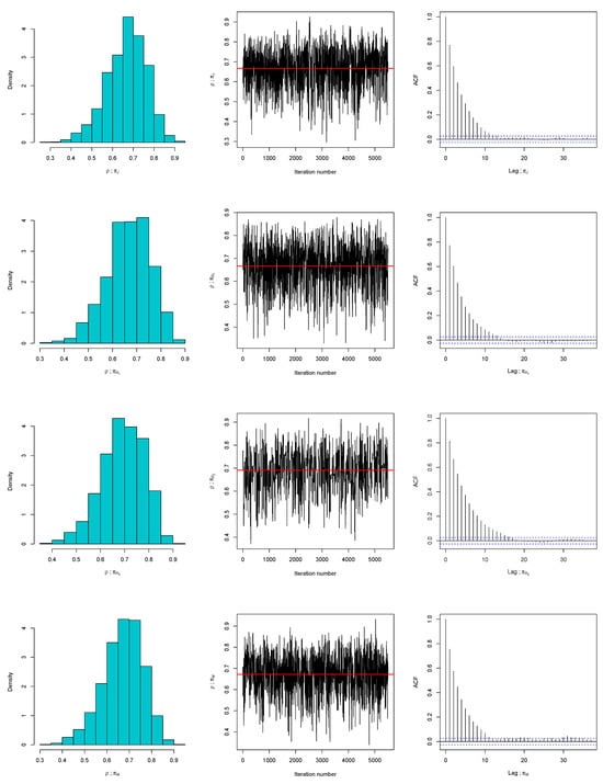
Figure 1. Diagnostic plots of the random walk MH algorithm for $\rho$ under ${\pi }_J$, ${\pi }_{R_1}$, ${\pi }_{R_2}$, and ${\pi }_M$ for the first data set.

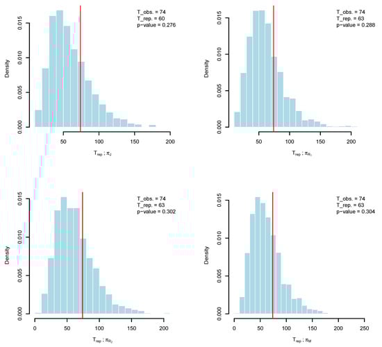
Figure 2. Histogram and kernel density of $T(\mathbf{x},\mathbf{y})$ along with its mean (red line) using ${\pi }_J$, ${\pi }_{R_1}$, ${\pi }_{R_2}$, and ${\pi }_M$ (clockwise from the top left) for the first data set.

Before presenting the Bayes estimates of $\rho$ obtained under different priors, we first provide the empirical estimate, defined as

$$\widehat{\rho }={\displaystyle \frac{1}{nm}}\sum _{i=1}^n\sum _{j=1}^{m}1\mathrm{I}(X_i\le Y_j).$$

Table 2 reports all estimates of $\rho$ together with their standard deviations (SDs) and 95% HPD credible intervals. Among them, the Bayes estimate based on ${\pi }_{R_2}$ outperforms the others by achieving the smallest SD, the narrowest 95% credible interval, and remaining closest to the empirical estimate. The Bayes estimate under ${\pi }_M$ ranks second in terms of proximity to the empirical estimate. Furthermore, the Bayes estimate using ${\pi }_{R_1}$ demonstrates better performance than both the Bayes estimate under ${\pi }_J$ and the ML estimate, as it yields a smaller SD and a shorter 95% credible interval.

Table 2. The summary of Bayesian estimates of $\rho$ for the first data.

Priors	Estimator	SD	95% CI
Empirical	0.6923	0.1120	(0.4726, 0.9120)
ML	0.6724	0.0916	(0.4929, 0.8519)
${\pi }_J$	0.6672	0.0954	(0.4543, 0.8345)
${\pi }_{R_1}$	0.6661	0.0914	(0.4721, 0.8280)
${\pi }_{R_2}$	0.6912	0.0878	(0.4966, 0.8333)
${\pi }_M$	0.6718	0.0906	(0.4705 0.8297)

6.2. Data-II

The second data set comprises the recorded lifetimes of steel specimens tested under 14 different stress levels. These data were originally reported by [28] and subsequently analyzed in greater detail by [26,29]. To illustrate our theoretical results, we focus on the lifetimes corresponding to a stress level of 32, which we denote by the stress variable X, with the following observed values: 1144, 231, 523, 474, 4510, 3107, 815, 6297, 1580, 605, 1786, 206, 1943, 935, 283, 1336, 727, 370, 1056, 413, 619, 2214, 1826, and 597. Similarly, the lifetimes measured at a stress level of 32.5 are treated as the strength variable Y, given by the following values: 4257, 879, 799, 1388, 271, 308, 2073, 227, 347, 669, 1154, 393, 250, 196, 548, 475, 1705, 2211, 975, and 2925. It is worth noting that the data set can be reasonably modeled using the geometric distribution, as confirmed by [26].

In a similar manner, Algorithms 1 and 2 are employed to draw posterior samples under the assumed priors and observed data, and to evaluate the adequacy of these priors, respectively. As illustrated in Figure 3, the posterior distribution of $\rho$ is well captured by a symmetric Gaussian proposal. Diagnostic plots further support this conclusion: the trace plots display stable fluctuations around the posterior means (marked by solid lines), and the corresponding autocorrelation functions (ACFs) decrease toward zero, indicating efficient mixing and low serial dependence. To assess prior suitability more thoroughly, Algorithm 2 is applied, with histograms and kernel density estimates of the discrepancy statistics shown in Figure 4. These results reveal that replicated samples from the Bayesian predictive distribution align closely with the observed data. Similarly, we run three MCMC chains and compute the Gelman–Rubin statistics. We found that $\widehat{R}$ is 1.0016 for ${\pi }_J$, 1.0003 for ${\pi }_{R_1}$, 1.0013 for ${\pi }_{R_2}$, and 1.00041 for ${\pi }_M$. Since all values of the statistic are well below the threshold of 1.05, the convergence of the MCMC is confirmed. Additionally, the posterior predictive p-values, $0.42$ for ${\pi }_J$, $0.406$ for ${\pi }_{R_1}$, $0.444$ for ${\pi }_{R_2}$, and $0.412$ for ${\pi }_M$, provide further evidence in favor of the compatibility of the proposed priors.

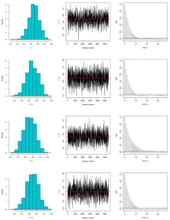
Figure 3. Diagnostic plots of the random walk MH algorithm for $\rho$ under ${\pi }_J$, ${\pi }_{R_1}$, ${\pi }_{R_2}$, and ${\pi }_M$ for the second data set.

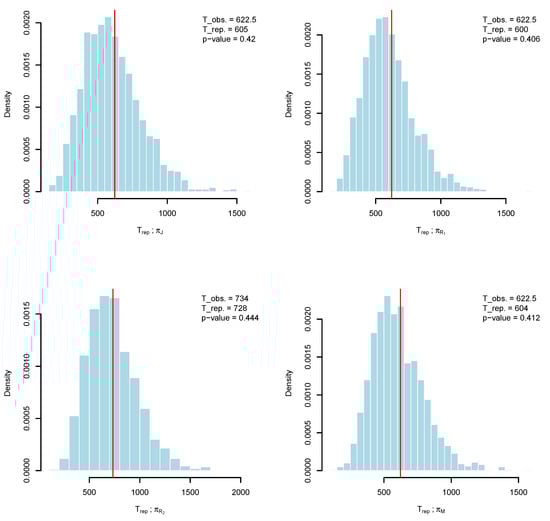
Figure 4. Histogram and kernel density of $T(\mathbf{x},\mathbf{y})$ along with its mean (red line) using ${\pi }_J$, ${\pi }_{R_1}$, ${\pi }_{R_2}$, and ${\pi }_M$ (clockwise from the top left) for the second data set.

Similarly, Table 3 presents the estimates of $\rho$ along with their standard deviations (SDs) and 95% HPD credible intervals. The ML and the Bayes estimates are relatively close to empirical estimate. On the other hand, the Bayes estimates obtained under ${\pi }_J$ and ${\pi }_M$ perform best, yielding the smallest SDs, the narrowest credible intervals, and the closest agreement with the empirical estimate. Furthermore, the Bayes estimates based on ${\pi }_{R_1}$ and ${\pi }_{R_2}$ also outperform the ML estimate, as they are associated with smaller SDs and shorter intervals.

Table 3. The summary of Bayesian estimates of $\rho$ for the second data.

Priors	Estimator	SD	95% CI
Empirical	0.5350	0.0935	(0.3518, 0.7182)
ML	0.5484	0.0891	(0.3739, 0.7228)
${\pi }_J$	0.5428	0.0766	(0.3898, 0.6880)
${\pi }_{R_1}$	0.5432	0.0805	(0.3819, 0.6887)
${\pi }_{R_2}$	0.5552	0.0888	(0.4079, 0.7103)
${\pi }_M$	0.5429	0.0798	(0.3824, 0.6954)

7. Conclusions

In this paper, we investigated maximum likelihood (ML) and Bayesian estimation procedures for the stress–strength parameter of the geometric distribution. We derived the ML estimator of $\rho$ and established its asymptotic distribution. For the Bayesian approach, we developed objective priors for $\rho$, namely Jeffreys, approximate reference, and matching priors. A key advantage of the Jeffreys prior is its invariance: the Bayes estimator of $\rho$ remains the same whether it is obtained directly in terms of $\rho$ or via a one-to-one transformation of the original model parameters. By contrast, reference and matching priors cannot in general be derived from those of the original parameters, since $\rho$ is a function of ${\theta }_1$ and ${\theta }_2$. This underscores the importance of constructing these priors directly in terms of $\rho$, ensuring that invariance is preserved upon transformation back to the original parameters.

We also examined the posterior distribution under these priors, noting that they are improper but lead to valid posteriors. Since closed-form Bayes estimates under the squared error loss function (SELF) are not available, we employed MCMC methods to compute them. Simulation studies demonstrated that the proposed Bayes estimators perform very well, with the matching prior generally outperforming both the other Bayesian approaches and the ML estimator, making it particularly suitable for practical use. Finally, two real data applications confirmed these findings: Bayesian estimates consistently outperformed ML estimates, with the matching prior yielding the best results overall, although the reference prior ${\rho }_{R_2}$ provided competitive performance in the first data set.

As in any study, a limitation of this work is that the proposed noninformative priors, including Jeffreys, reference, and matching priors, for the geometric stress–strength reliability may suffer from stability issues when the parameters lie close to the boundaries of the parameter space. This motivates us to further investigate such cases in future research. In addition, the methodology developed in this paper can be extended to other settings, such as record values or type-II censored data, which are frequently encountered in real applications, particularly in hydrology and lifetime studies. Under these two schemes, the likelihood remains tractable, making the use of the developed priors feasible.

References

- Kundu, D.; Gupta, R.D. Estimation of P(Y < X) for generalized exponential distribution. Metrika 2005, 61, 291–308. [Google Scholar]
- Kumar, I.; Kumar, K. On estimation of P(V < U) for inverse pareto distribution under progressively censored data. Int. J. Syst. Assur. Eng. Manag. 2022, 13, 189–202. [Google Scholar]
- Khan, M.; Khatoon, B. Statistical inferences of R=P(X < Y) for exponential distribution based on generalized order statistics. Ann. Data Sci. 2020, 7, 525–545. [Google Scholar]
- Yadav, A.S.; Singh, S.; Singh, U. Bayesian estimation of stress–strength reliability for lomax distribution under type-II hybrid censored data using asymmetric loss function. Life Cycle Reliab. Saf. Eng. 2019, 8, 257–267. [Google Scholar] [CrossRef]
- Sun, D.; Ghosh, M.; Basu, A.P. Bayesian analysis for a stress-strength system under noninformative priors. Can. J. Stat. 1998, 26, 323–332. [Google Scholar]
- Kang, S.G.; Lee, W.D.; Kim, Y. Objective bayesian analysis for generalized exponential stress–strength model. Comput. Stat. 2021, 36, 2079–2109. [Google Scholar] [CrossRef]
- Abbas, K.; Tang, Y. Objective bayesian analysis of the Fréchet stress–strength model. Stat. Probab. Lett. 2014, 84, 169–175. [Google Scholar] [CrossRef]
- Barbiero, A. Inference on reliability of stress-strength models for Poisson data. J. Qual. Reliab. Eng. 2013, 2013, 530530. [Google Scholar] [CrossRef]
- Obradovic, M.; Jovanovic, M.; Milošević, B.; Jevremović, V. Estimation of P(X ≤ Y) for geometric-poisson model. Hacet. J. Math. Stat. 2015, 44, 949–964. [Google Scholar]
- Ahmad, K.E.; Fakhry, M.E.; Jaheen, Z.F. Bayes estimation of P(Y > X) in the geometric case. Microelectron. Reliab. 1995, 35, 817–820. [Google Scholar] [CrossRef]
- Maiti, S.S. Estimation of P(X ≤ Y) in the geometric case. J. Indian Stat. Assoc. 1995, 33, 87–91. [Google Scholar]
- Mohamed, M. Inference for reliability and stress-strength for geometric distribution. Sylwan 2015, 159, 281–289. [Google Scholar]
- Mohamed, M. Estimation of R for geometric distribution under lower record values. J. Appl. Res. Technol. 2020, 18, 368–375. [Google Scholar] [CrossRef]
- Datta, G.S.; Ghosh, M. On the invariance of noninformative priors. Ann. Stat. 1996, 24, 141–159. [Google Scholar] [CrossRef]
- Dong, G.; Shakhatreh, M.K.; He, D. Bayesian analysis for the shannon entropy of the lomax distribution using noninformative priors. J. Stat. Comput. Simul. 2024, 94, 1317–1338. [Google Scholar] [CrossRef]
- Sen, P.K.; Singer, J.M. Large Sample Methods in Statistics: An Introduction with Applications; Chapman & Hall: London, UK, 1993. [Google Scholar]
- Berger, J.O.; Bernardo, J.M. Ordered group reference priors with application to the multinomial problem. Biometrika 1992, 79, 25–37. [Google Scholar] [CrossRef]
- Bernardo, J.M. Reference analysis. Handb. Stat. 2005, 25, 17–90. [Google Scholar]
- Bernardo, J.M.; Smith, A.F. Bayesian Theory; John Wiley & Sons: Hoboken, NJ, USA, 2009; Volume 405. [Google Scholar]
- Welch, B.L.; Peers, H. On formulae for confidence points based on integrals of weighted likelihoods. J. R. Stat. Soc. Ser. B (Methodol.) 1963, 25, 318–329. [Google Scholar] [CrossRef]
- Datta, G.S.; Ghosh, J.K. On priors providing frequentist validity for Bayesian inference. Biometrika 1995, 82, 37–45. [Google Scholar] [CrossRef]
- Neal, P.; Roberts, G. Optimal scaling for random walk metropolis on spherically constrained target densities. Methodol. Comput. Appl. Probab. 2008, 10, 277–297. [Google Scholar] [CrossRef]
- Guttman, I. The use of the concept of a future observation in goodness-of-fit problems. J. R. Stat. Soc. Ser. B (Methodol.) 1967, 29, 83–100. [Google Scholar] [CrossRef]
- Meng, X.-L. Posterior predictive p-values. Ann. Stat. 1994, 22, 1142–1160. [Google Scholar] [CrossRef]
- Pedersen, M.M.; Mouritsen, O.Ø; Hansen, M.R.; Andersen, J.G.; Wenderby, J. Comparison of post-weld treatment of high-strength steel welded joints in medium cycle fatigue. Weld. World 2010, 54, R208–R217. [Google Scholar] [CrossRef]
- Nayal, A.S.; Singh, B.; Tyagi, A.; Chesneau, C. Classical and bayesian inferences on the stress-strength reliability R=P[Y < X < Z] in the geometric distribution setting. AIMS Math. 2023, 8, 20679–20699. [Google Scholar]
- Brooks, S.P.; Gelman, A. General Methods for Monitoring Convergence of Iterative Simulations. J. Comput. Graph. Stat. 1998, 7, 434–455. [Google Scholar] [CrossRef]
- Kimber, A. Exploratory data analysis for possibly censored data from skewed distributions. J. R. Stat. Soc. Ser. C Appl. Stat. 1990, 39, 21–30. [Google Scholar] [CrossRef]
- Crowder, M. Tests for a family of survival models based on extremes. In Recent Advances in Reliability Theory; Birkhäuser: Boston, MA, USA, 2000. [Google Scholar]
Disclaimer/Publisher’s Note: The statements, opinions and data contained in all publications are solely those of the individual author(s) and contributor(s) and not of MDPI and/or the editor(s). MDPI and/or the editor(s) disclaim responsibility for any injury to people or property resulting from any ideas, methods, instructions or products referred to in the content. |
© 2025 by the author. Licensee MDPI, Basel, Switzerland. This article is an open access article distributed under the terms and conditions of the Creative Commons Attribution (CC BY) license (https://creativecommons.org/licenses/by/4.0/).