Invariant Sets, Global Dynamics, and the Neimark–Sacker Bifurcation in the Evolutionary Ricker Model

Abstract

In this paper, we study the local, global, and bifurcation properties of a planar nonlinear asymmetric discrete model of Ricker type that is derived from a Darwinian evolution strategy based on evolutionary game theory. We make a change of variables to both reduce the number of parameters as well as bring symmetry to the isoclines of the mapping. With this new model, we demonstrate the existence of a forward invariant and globally attracting set where all the dynamics occur. In this set, the model possesses two symmetric fixed points: the origin, which is always a saddle fixed point, and an interior fixed point that may be globally asymptotically stable. Moreover, we observe the presence of a supercritical Neimark–Sacker bifurcation, a phenomenon that is not present in the original non-evolutionary model.

1. Introduction

The standard one-dimensional Ricker equation refers to the discrete population model $x_{n+1}=r{x}_n{e}^{-a{x}_n}$ with parameters r, a and an initial condition $x_0>0$. This model is named after Ricker’s work fitting the parameters to reproductive curves for fish populations, including the Pacific Herring, Pink Salmon, Coho Salmon, and Sockeye Salmon, among others [1]. From a mathematical perspective, an increase in r leads to period doubling bifurcations and eventually chaos [2]. In a controlled laboratory, such bifurcations were observed in Tribolium flour beetles [3]. However, as noted in [4], ecologists have rarely observed chaos in animal populations in nature. This suggested that, in a real-world setting, one-dimensional models such as the Ricker model are missing important factors.

In a series of papers [5,6,7,8,9,10,11], Jim Cushing, along with some coauthors, established the foundations of discrete evolutionary models using the idea of Darwinian evolution strategy [12] based on evolutionary game theory [13]. These evolutionary game models differ in significant ways from classical theory, while classical games focus on strategies that optimize players’ payoffs, evolutionary games emphasize strategies that persist over time. Through births and deaths, players come and go, but their strategies are passed down from generation to generation [14].

The first appearance of evolutionary models in discrete dynamical systems was in [6], applied to the classic Beverton–Holt (discrete logistic) model. Using standard methods for modeling evolution, the one-dimensional model becomes a planar system of coupled difference equations, consisting of a Beverton–Holt type equation for the population dynamics and a difference equation for the dynamics of the mean phenotype trait. By studying the case when the trait equation uncouples from the population dynamic equation, Cushing was able to obtain criteria under which the evolutionary system has globally asymptotically stable equilibria or periodic solutions.

Recently, Ch-Chaoui and Moknni [15] studied the coupled case of the evolutionary Beverton–Holt model and discussed the existence of the positive fixed point, exploring its asymptotic stability. Under certain parametric conditions, they discussed the Neimark–Sacker bifurcation, a phenomenon that does not occur in the classic Beverton–Holt model.

This strategy of deriving an evolutionary model was extended to more general discrete models [7,9,11]. In particular, models with the Allee effect [10], models of Ricker type [8,16,17] and multi-species models [17,18,19].

In all these studies, the main mathematical goals are to find and classify the stability of equilibria, identify bifurcations, and when possible, describe the global dynamics of the models. In the case of a lone locally stable equilibrium, a great deal of studying has been performed on whether this fixed point is also globally attracting. While there exist many general theorems on global stability in one-dimensional mappings [20,21,22], this problem is more difficult in higher dimensions. Some successful examples of establishing global stability in higher dimensions include of those of monotone and mixed-monotone systems [19,23,24,25,26,27]. For non-monotone systems, singularity curves [28,29,30,31] have also been used to establish global stability if the mapping satisfies certain topological constraints [32,33,34,35]; these curves will also play an important role in the present work. However, in full generality, the question of global stability even in the planar case is far from understood. Some open problems and conjectures in two-dimensions may be found in [36].

In a recent paper [37], the author proposed a series of open problems and conjectures concerning the global stability of the following evolutionary discrete model of Ricker type for a single-species x (with a single mean trait u and individual trait v)

$$\left\{\begin{array}{c}x(t+1)=x\left(t\right)e^{\alpha \left(t\right)-{\displaystyle \frac{u^2\left(t\right)}{2}}-c_{0}x\left(t\right)}\hfill \\ u(t+1)=(1-{\sigma }^2)u\left(t\right)-c_1{\sigma }^{2}x\left(t\right)\hfill \end{array}\right.,$$

(1)

where the parameters $\alpha \left(t\right)$ are the sequence of growth rates (which are functions of the trait), $c_0$ is the competition coefficient, ${\sigma }^2\ge 0$ is the speed of evolution, and $c_1$ is the sensitivity of the competition. A complete derivation and explanation of these parameters may be found in [8].

Notice that if

$$\alpha \left(t\right)=\alpha ,\mathrm{for}\mathrm{all}t=0,1,2,\dots ,$$

then Model (1) is autonomous whereas if

$$\alpha (t+p)=\alpha \left(t\right),\mathrm{for}\mathrm{all}t=1,2,\dots \mathrm{and}\mathrm{some}\mathrm{integer}p>1,$$

then Model (1) is $p$-periodic.

We remark that the first Equation in (1) is known in the literature as the inherent fertility equation while the second equation is the trait equation. Other names for the trait equation include the canonical equation for evolution [38], Lande’s Equation [39,40] and Fisher’s Equation [41].

In the autonomous case, for the parameter values $1<{\sigma }^2<2$, Model (1) is mixed-monotone, and the following result addresses the global stability of the model:

Theorem 1 

([19]). Let $\alpha \left(t\right)=\alpha >0$ for all $t=0,1,2\dots$, such that $0<\alpha <1$, $1<{\sigma }^2<2$, and $c_1\ne 0$. Then, the interior equilibrium point $E^{\ast }=(x^{\ast },-c_1{x}^{\ast })$ of Model (1) is globally asymptotically stable if it is locally asymptotically stable, where $x^{\ast }=\left(-c_0+\sqrt{c_0^2+2\alpha c_1^2}\right)/c_1^2$.

The conditions of local stability required in Theorem 1 are

$$c_0(2+{\sigma }^2)x^{\ast }<2((\alpha -1){\sigma }^2+2)$$

and

$$c_0(1+{\sigma }^2)x^{\ast }>(2\alpha -1){\sigma }^2,$$

with $\alpha >0$, ${\sigma }^2<2$ and $c_1\ne 0$ as stated in Theorem 2.1 in [19]. In particular, Theorem 1 shows that local stability implies global stability in the parameter range $1<{\sigma }^2<2$. In this paper, we address the case of $0<{\sigma }^2<1$, where the mapping is no longer mixed-monotone and new techniques are needed.

In this paper, we solve one of the conjectures presented in [37]; specifically, we demonstrate the global stability of the interior fixed point of Model (1) when $0<\alpha <1$ and ${\sigma }^2<1$, thereby completing Theorem 1 in the global stability approach. Furthermore, we go beyond the concept of global stability by characterizing the invariant manifolds of the fixed points and also the bifurcation of the interior fixed point. As is seen in populations in nature, we will prove that this model does not undergo a period doubling cascade to chaos.

In order to achieve these goals, in Section 2 we make a change in the variables in Model (1) and write a simplified model that will help us understand both the local and global properties of the original model.

Using the concept of critical curves [29], in Section 3 we identify a forward-invariant and globally attracting subset under the action of the system’s mapping. Subsequently, in Section 4 and Section 5, we analyze the stability and bifurcation of the fixed points within this invariant set. Finally, in the last two sections, we provide the conclusion and discuss future work.

We believe that the techniques followed in this paper will aid in the study of similar models, namely, the use of critical curves and isoclines for identifying the maximal invariant set where all the dynamics take place; the characterization of the invariant (stable and unstable) manifolds that attract all orbits in the invariant set; and the classification of the Neimark–Sacker bifurcation using a geometric argument, which, to our knowledge, is the first time that a supercritical case has been classified via such an argument.

2. Notation and Preliminaries

By using a change in variables in Model (1), it is possible to reduce the number of parameters involved, thereby simplifying the study.

Let us consider the autonomous system

$$\begin{array}{c}\hfill \left\{\begin{array}{c}{w}_{n+1}=w_n{e}^{\alpha -{\displaystyle \frac{1}{2}}{u}_n^2-c_0{w}_n}\hfill \\ u_{n+1}=(1-{\sigma }^2)u_n-c_1{\sigma }^2{w}_n\hfill \end{array}\right.,\end{array}$$

(2)

equivalent to Model (1), for $\alpha >0$, $c_0\ne 0$, $c_1\ne 0$, and $0<{\sigma }^2<1$.

Let $x_n=c_0{w}_n$ and $y_n=-{\displaystyle \frac{c_0}{c_1}}{u}_n$. Then,

$$\begin{array}{cc}\hfill x_{n+1}& =c_0{w}_{n+1}\hfill \\ & =c_0{w}_n{e}^{\alpha -{\displaystyle \frac{1}{2}}{u}_n^2-c_0{w}_n}=x_n{e}^{\alpha -{\displaystyle \frac{1}{2}}{u}_n^2-x_n}\hfill \\ & =x_n{e}^{\alpha -{\displaystyle \frac{c_1^2}{2c_0^2}}{y}_n^2-x_n}\hfill \end{array}$$

and

$$\begin{array}{cc}\hfill y_{n+1}& =-{\displaystyle \frac{c_0}{c_1}}{u}_{n+1}\hfill \\ & =-{\displaystyle \frac{c_0}{c_1}}(1-{\sigma }^2)u_n+{\sigma }^2{c}_0{w}_n\hfill \\ \hfill & =(1-{\sigma }^2)y_n+{\sigma }^2{x}_n.\hfill \end{array}$$

Hence, the properties of Model (2) are the same as the following system

$$\begin{array}{c}\hfill \left\{\begin{array}{c}{x}_{n+1}=x_n{e}^{\alpha -{\displaystyle \frac{c_1^2}{2c_0^2}}{y}_n^2-x_n}\hfill \\ y_{n+1}=(1-{\sigma }^2)y_n+{\sigma }^2{x}_n\hfill \end{array}\right..\end{array}$$

(3)

Let F be the mapping representing Model (3) given by

$$F(x,y)=\left(f(x,y),g(x,y)\right)=\left(x{e}^{\alpha -x-\beta y^2},(1-{\sigma }^2)y+{\sigma }^{2}x\right),$$

where $\beta ={\displaystyle \frac{c_1^2}{2c_0^2}}$ for $x\ge 0$.

In the following sections, we will study the dynamics of invariant sets under the mapping F representing Model (3), as well as some properties of the fixed points of F.

3. Critical Curves and Invariant Sets

We start by examining the preimages of F representing Model (3). Initially, we follow the work of [29]. They assume there is a mapping F that is a noninvertible planar mapping whose preimage at any point consists of a finite number of isolated points. They then divide the plane into regions $Z_k$, where $(x,y)\in Z_k$ if and only if $(x,y)$ has k preimages under F. Following their notation, the boundaries of these regions is denoted by $LC$, with preimage $L{C}_{-1}=F^{-1}\left(LC\right)$. For smooth mappings, they show that $L{C}_{-1}$ can be determined by the set of points where the determinant of the Jacobian of F vanishes, in which case $LC=F\left(L{C}_{-1}\right)$.

For the map F representing Model (3), we will show that $LC$ separates the first and fourth quadrant into two distinct regions $Z_2$ and $Z_0$, as is illustrated in Figure 1. All points in the interior of the shaded region have two distinct preimages while points in the unshaded region have no preimage, as will be shown in Theorem 2.

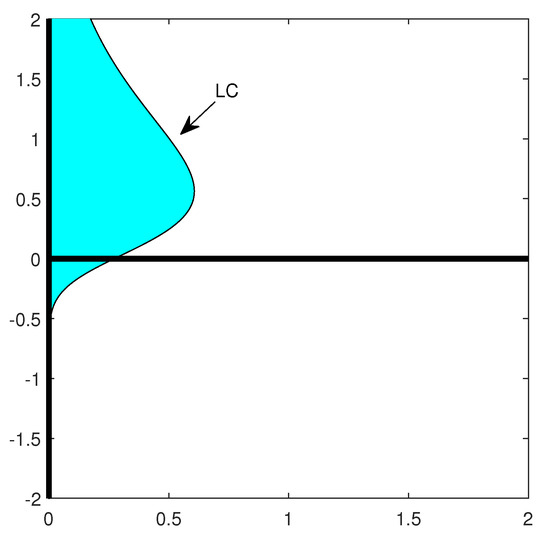
Figure 1. The graph of $LC$ separates the plane into two distinct regions. All points in the interior of the shaded region have two distinct preimages. Points in the unshaded region have no preimage.

The Jacobian of the mapping F is given by

$$DF=J(x,y)=\left[\begin{array}{cc}(1-x)e^{\alpha -x-\beta y^2}& -2\beta xy{e}^{\alpha -x-\beta y^2}\\ {\sigma }^2& 1-{\sigma }^2\end{array}\right].$$

Then,

$$det\left(J(x,y)\right)=\left((1-x)(1-{\sigma }^2)+2\beta {\sigma }^{2}xy\right)e^{\alpha -x-\beta y^2}$$

and this determinant vanishes along the graph of

$$y=\varphi \left(x\right)={\displaystyle \frac{(x-1)(1-{\sigma }^2)}{2\beta {\sigma }^{2}x}}$$

with $x>0$. Consequently, $L{C}_{-1}=\{(x,y)\in {\mathbb{R}}^2:y=\varphi \left(x\right),x>0\}$ and $LC=F\left(L{C}_{-1}\right)$. We now look at the geometry of $L{C}_{-1}$ and $LC$ in more detail.

Lemma 1. 

Let $\alpha ,\beta >0$, and let $\sigma \in (0,1)$. Then the graph of $L{C}_{-1}$ is a monotone increasing and concave curve. It has a vertical asymptote at $x=0$ and a horizontal asymptote at $y={\displaystyle \frac{1-{\sigma }^2}{2\beta {\sigma }^2}}$.

Proof. 

The first claim follows by calculating derivatives of $\varphi$. The asymptotes follow by taking the appropriate limits. □

Lemma 2. 

Let $\alpha ,\beta >0$, and let $\sigma \in (0,1)$. Then, the curve $LC$ can be decomposed into curves ${\gamma }_1$ from $(0,-\infty )$ to $(e^{\alpha -1},{\sigma }^2)$ and ${\gamma }_2$ from $(0,\infty )$ to $(e^{\alpha -1},{\sigma }^2)$ where ${\gamma }_1$ is strictly increasing and ${\gamma }_2$ is strictly decreasing. At the intersection point $(e^{\alpha -1},{\sigma }^2)$, $LC$ has a vertical tangent line.

Proof. 

The curve $LC$ has parametrization

$$\mathbf{r}\left(t\right)=\left(f_1\left(t\right),g_1\left(t\right)\right)=\left(t{e}^{\alpha -t-\beta \varphi {\left(t\right)}^2},(1-{\sigma }^2)\varphi \left(t\right)+{\sigma }^{2}t\right)$$

for $t\in (0,\infty )$. We claim that ${\gamma }_1$ consists of the portion of $r\left(t\right)$ for $t\in (0,1]$ and that ${\gamma }_2$ consists of the part with $t\in [1,\infty )$. We calculate

$$\begin{array}{cc}\hfill {\displaystyle \frac{d{f}_1\left(t\right)}{dt}}& =e^{\alpha -t-\beta \varphi {\left(t\right)}^2}\left(1-t-2\beta t\varphi \left(t\right){\varphi }^{\prime }\left(t\right)\right)\hfill \end{array}$$

and

$$\begin{array}{cc}\hfill {\displaystyle \frac{d{g}_1\left(t\right)}{dt}}& =(1-{\sigma }^2){\varphi }^{\prime }\left(t\right)+{\sigma }^2.\hfill \end{array}$$

It is clear that ${\displaystyle \frac{d{g}_1}{dt}}>0$ for all t. Also, for $t<1$, both $1-t>0$ and $-\varphi \left(t\right){\varphi }^{\prime }\left(t\right)>0$, so ${\displaystyle \frac{d{f}_1}{dt}}>0$ for $t\in (0,1)$. Similarly, for $t>1$, both $1-t<0$ and $-\varphi \left(t\right){\varphi }^{\prime }\left(t\right)<0$, so ${\displaystyle \frac{d{f}_1}{dt}}<0$ for $t>1$. Since ${\displaystyle \frac{d{f}_1\left(t\right)}{dt}}$ vanishes at $t=1$, the curve has a vertical tangent line at $\mathbf{r}\left(1\right)=(e^{\alpha -1},{\sigma }^2)$. □

We remark that the relative positions of the critical curves as well their properties, as described in Lemmas 1 and 2, are clearly illustrated in Figure 2. As we can observe, the critical curves do not intersect, and there are points on the left side of $LC$ with the same y component that have two distinct preimages symmetric about a point on the critical curve $L{C}_{-1}$.

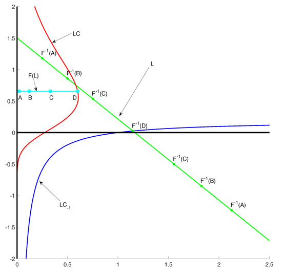
Figure 2. Graphs of $LC$, $L{C}_{-1}=F^{-1}\left(LC\right)$, and a line L with slope $-{\displaystyle \frac{{\sigma }^2}{1-{\sigma }^2}}$ and its image under F are shown. The image of the line is symmetric about the point on $L{C}_{-1}$, where each point to the lower right of $L{C}_{-1}$ may be identified with a point to the upper left, as they have the same dynamics. To illustrate this, four points $A,B,C,D$ are shown on $F\left(L\right)$, with their preimages under F marked on L. For instance, the two points marked $F^{-1}\left(A\right)$ both map to A and share the same future thereafter. The values used in this graph are $\alpha ={\displaystyle \frac{1}{2}}$, $\beta =2$, $\sigma ={\displaystyle \frac{3}{4}}$. Lemmas 1, 2, and Theorem 2 have shown that this depiction is typical for all lines with this slope for any $\alpha \in (0,1)$, $\beta >0$, and ${\sigma }^2\in (0,1)$.

Before we proceed with the analysis of our model, let us take an overall look at a concrete example:

Example 1. 

Let $\alpha ={\displaystyle \frac{1}{2}}$, $\beta =2$ and $\sigma ={\displaystyle \frac{3}{4}}$. Then, the critical curve $L{C}_{-1}=\{(x,y)\in {\mathbb{R}}^2:y={\displaystyle \frac{7(x-1)}{36x}}\}$ and a parametrization of $LC$ is written as

$$r\left(t\right)=\left(f_1\left(t\right),g_1\left(t\right)\right)=\left(t{e}^{-{\displaystyle \frac{49{(t-1)}^2}{648t^2}}-t+{\displaystyle \frac{1}{2}}},{\displaystyle \frac{324t^2+49t-49}{576t}}\right),t\in (0,\infty ).$$

Clearly, the conclusion of the precedent theorem is satisfied since $g_1^{\prime }\left(t\right)={\displaystyle \frac{324t^2+49}{576t^2}}$ and

$$f_1^{\prime }\left(t\right)=-(t-1){\displaystyle \frac{\left(324t^2+49\right)}{324t^2}}{e}^{-{\displaystyle \frac{49{(t-1)}^2}{648t^2}}-t+{\displaystyle \frac{1}{2}}}.$$

A representation of the graphs of $L{C}_{-1}$ and $LC$ is shown in Figure 2. As one can observe the curve, $LC$ divides the first and fourth quadrant into two distinct regions. Now, let $A=\left({\displaystyle \frac{1}{50}},{\displaystyle \frac{21}{32}}\right)$, $B=\left({\displaystyle \frac{3}{25}},{\displaystyle \frac{21}{32}}\right)$, $C=\left({\displaystyle \frac{1}{3}},{\displaystyle \frac{21}{32}}\right)$, and $D=\left(\overline{x},{\displaystyle \frac{21}{32}}\right)$, all taken with the same y-coordinate, where $\overline{x}$ is the intersection of the line $y={\displaystyle \frac{21}{32}}$ and the curve $LC$. To calculate $\overline{x}$, we use the parametrization $g_1\left(t\right)$ and solve ${\displaystyle \frac{324{\overline{t}}^2+49\overline{t}-49}{576\overline{t}}}={\displaystyle \frac{21}{32}}$, yielding $\overline{t}={\displaystyle \frac{329}{648}}+{\displaystyle \frac{7\sqrt{3505}}{648}}$. Then, $\overline{x}=f_1\left(\overline{t}\right)\approx 0.5998$.

A forward computation shows that the first three points have two preimages as follows

$$F^{-1}\left(A\right)\approx \{(0.25026,1.17824),(2.12565,-1.23297)\}$$

$$F^{-1}\left(B\right)\approx \{(0.50788,0.84702),(1.81746,-0.83673)\}$$

$$F^{-1}\left(C\right)\approx \{(0.75425,0.53025),(1.55036,-0.49333)\}$$

while D has a single preimage on $L{C}_{-1}$ given approximately by

$$F^{-1}\left(D\right)\approx (1.14725,0.02496).$$

All of the preimages fall on the line $y={\displaystyle \frac{3}{2}}-{\displaystyle \frac{9}{7}}x$, marked as L in Figure 2.

The precedent example motivates the following result:

Theorem 2. 

Let $\alpha ,\beta >0$, and let $\sigma \in (0,1)$. Then, the curve $LC$ divides the first and fourth quadrant into two regions. For the region adjacent to the y-axis, each point with positive x coordinate has two distinct preimages. The other region is not in the range of F.

Proof. 

The conclusion that $LC$ divides the plane into two regions follows from Lemma 2. To prove the remaining claim, we consider the set of lines with slope $-{\displaystyle \frac{{\sigma }^2}{1-{\sigma }^2}}$, whose image we will show is a horizontal line. Let

$$L_{(x,y)}=\left\{(x-(1-{\sigma }^2)xt,y+{\sigma }^{2}xt):-\infty <t\le {\displaystyle \frac{1}{1-{\sigma }^2}}\right\}.$$

Since $L{C}_{-1}$ is monotonically increasing, each line intersects $L{C}_{-1}$ exactly once, so it suffices to consider the set of lines $L_{(x,\varphi (x\left)\right)}$.

Noting that $2\beta x\varphi \left(x\right){\sigma }^2=(x-1)(1-{\sigma }^2)$, we have

$$\begin{array}{cc}\hfill f\left(L_{(x,\varphi (x\left)\right)}\right)& =x\left(1-(1-{\sigma }^2)t\right)e^{\alpha -x+(1-{\sigma }^2)xt-\beta {\left(\varphi \left(x\right)\right)}^2-2\beta {\sigma }^2\varphi \left(x\right)xt-\beta {\sigma }^4{x}^2{t}^2}\hfill \\ & =x{e}^{\alpha -x-\beta {\left(\varphi \left(x\right)\right)}^2}\left(1-(1-{\sigma }^2)t\right)e^{(1-{\sigma }^2)xt-2\beta {\sigma }^2\varphi \left(x\right)xt-\beta {\sigma }^4{x}^2{t}^2}\hfill \\ & =f(x,\varphi \left(x\right))\left(1-(1-{\sigma }^2)t\right)e^{(1-{\sigma }^2)xt-(x-1)(1-{\sigma }^2)t-\beta {\sigma }^4{x}^2{t}^2}\hfill \\ & =f(x,\varphi \left(x\right))\left(1-(1-{\sigma }^2)t\right)e^{(1-{\sigma }^2)t-\beta {\sigma }^4{x}^2{t}^2}\hfill \end{array}$$

and

$$\begin{array}{cc}\hfill g\left(L_{(x,\varphi (x)}\right))& =\varphi \left(x\right)+{\sigma }^{2}xt+{\sigma }^2\left(x-(1-{\sigma }^2)xt-\varphi \left(x\right)-{\sigma }^{2}xt\right)\hfill \\ & =\varphi \left(x\right)+{\sigma }^{2}xt+{\sigma }^{2}x-{\sigma }^{2}xt+{\sigma }^{4}xt-{\sigma }^2\varphi \left(x\right)-{\sigma }^{4}xt\hfill \\ & =\varphi \left(x\right)+{\sigma }^{2}x-{\sigma }^2\varphi \left(x\right)\hfill \\ & =g(x,\varphi (x\left)\right).\hfill \end{array}$$

Thus, the image of the line $L_{(x,\varphi (x\left)\right)}$ is horizontal since the y coordinate is fixed at $g(x,\varphi (x\left)\right)$. To study what happens to the x coordinate, we look at the multiplicative factor

$$h\left(t\right)=\left(1-(1-{\sigma }^2)t\right)e^{(1-{\sigma }^2)t-\beta {\sigma }^4{x}^2{t}^2}.$$

When $t=0$, $h\left(t\right)=1$, so the x coordinate $f\left(L_{(x,\varphi (x\left)\right)}\right)$ is $f(x,\varphi (x\left)\right)$, i.e., it lies on $LC$. Since

$$h^{\prime }\left(t\right)=\left(-2\beta {\sigma }^4{x}^{2}t(1-(1-{\sigma }^2)t)-{(1-{\sigma }^2)}^{2}t\right)e^{(1-{\sigma }^2)t-\beta {\sigma }^4{x}^2{t}^2},$$

h is increasing for $t<0$ and decreasing for $0<t\le {\displaystyle \frac{1}{1-{\sigma }^2}}$. Consequently, the image of the line is always to the left of $LC$. Moreover, it traces the line from $\left(0,g(x,\varphi (x\left)\right)\right)$ to $\left(f(x,\varphi (x\left)\right),g(x,\varphi (x\left)\right)\right)$ exactly once for $-\infty <t<0$, and the image traces the horizontal line in the reverse direction for $0<t\le {\displaystyle \frac{1}{1-{\sigma }^2}}$. □

To summarize, every point to the left of $LC$ with positive x coordinate has exactly two preimages, one to the upper left of $L{C}_{-1}$ and one to its lower right. The map’s orientation is preserving in the upper left and the orientation is reversing in the lower right, best seen by the images of the lines $L_{(x,\varphi (x\left)\right)}$. From the symmetry of the image of the mapping about these line, we only need to consider the mapping F restricted to $Z_2\cup LC$. In fact, for sufficiently large n the y coordinate of $F^n$ is always between 0 and 1. This motivates the final theorem of this subsection.

Theorem 3. 

Let U denote the closed region bounded by the coordinate axes, the curve $LC$, and the line $y=1$. Let $\alpha \in (0,1)$, $\beta >0$, and $\sigma \in (0,1)$. Then, U is forward invariant under F, $F:U\to U$ is injective, and U is globally attracting.

Proof. 

First, we establish that U is invariant. Let $(x,y)\in U$. From the discussion above, $f(x,y)$ always lies to the left of $LC$, so we must prove that $(x,y)\in U$ implies $g(x,y)=(1-{\sigma }^2)y+{\sigma }^{2}x\in [0,1]$. Since x lies to the left of $LC$, we must have $0\le x<1$. Then, we have

$$0\le (1-{\sigma }^2)y+{\sigma }^{2}x\le 1-{\sigma }^2+{\sigma }^2\le 1$$

establishing that U is forward invariant.

The graph of $L{C}_{-1}$ crosses the x-axis at the point $(1,0)$. Thus, the graph of $L{C}_{-1}$ is always to the right of U. Consequently, at most one preimage of a point in U can lie in U since the other preimage must lie to the lower right of $L{C}_{-1}$. This shows that the restriction of F to U is injective.

Finally, we show U is globally attracting. First, observe that the first quadrant is forward invariant. Note that if $y<0$, then $g(x,y)=y+{\sigma }^2(x-y)>y$. If $F^n(x,y)$ never maps to the first quadrant, then the set of y coordinates of ${\left\{F^n(x,y)\right\}}_{n\in \mathbb{Z}}$ is a bounded and strictly monotone increasing sequence that must converge to a value $y^{\ast }\le 0$. If $y^{\ast }<0$, this is a contradiction since there is no invariant set of points with fixed y negative coordinate by the inequality above in g. Consequently, either the sequence ${\left\{F^n(x,y)\right\}}_{n\in \mathbb{Z}}$ has its y coordinate approach 0, or it eventually maps to a positive value.

Thus, it suffices to consider $(x,y)$ with $y\ge 0$. We will show there exists an integer k such that the y coordinate of $F^k(x,y)$ is less than or equal to 1. Since $f(x,y)<1$ (since the x coordinate lies to the left of $LC$), if $g(x,y)>1$, then we have

$$g\left(f(x,y),g(x,y)\right)=g(x,y)+{\sigma }^2\left(f(x,y)-g(x,y)\right)<g(x,y).$$

If the y value of $F^n(x,y)$ always exceeds 1, then similar to before, the y coordinates of ${\left\{F^n(x,y)\right\}}_{n\in {\mathbb{Z}}^{+}}$ form a bounded and strictly monotone decreasing sequence that must converge to a value $y^{\ast }\ge 1$. As there is no invariant set with $y^{\ast }>1$, the theorem is proved. □

In Figure 3, we depict a prototype of the closed invariant region U mentioned in Theorem 3, where the mapping F is injective. As is clearly shown, only a portion of the critical curve $LC$ on the boundary of this region will move strictly according to the values of the parameters, while the remaining three segments of the boundary are defined by conditions that do not depend on the parameters. This region U is crucial for the global analysis of the model, as all the dynamics of (3) occur within it.

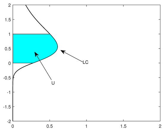
Figure 3. The region U bounded by $x=0$, $y=0$, $y=1$, and the curve $LC$, where the parameters values are $\alpha ={\displaystyle \frac{1}{2}}$, $\beta =2$, and $\sigma ={\displaystyle \frac{3}{4}}$. This region is forward invariant, globally attracting, and the restriction of F to U is injective, as proved in Theorem 3. Lemma 2 shows that the general shape of region U is typical.

4. Isoclines and Fixed Points

Let us denote the restriction of F to U, mentioned in the previous section, by $F_U$. The isoclines of $F(x,y)=\left(f(x,y),g(x,y)\right)$ are given by the set of points that satisfy $f(x,y)=x$ and the points that satisfy $g(x,y)=y$. For $F_U:U\to U$ with

$$F_U(x,y)=\left(x{e}^{\alpha -x-\beta y^2},(1-{\sigma }^2)y+{\sigma }^{2}x\right)$$

the isoclines can be broken into three distinct sets:

$$\begin{array}{cc}\hfill I_1& =\left\{\right(x,y)\in U:y=x\},\hfill \\ \hfill I_2& =\{(x,y)\in U:x+\beta y^2=\alpha \}\hfill \end{array}$$

and

$$\begin{array}{cc}\hfill I_3& =\left\{\right(x,y)\in U:x=0\}.\hfill \end{array}$$

From the isoclines, we easily obtain that there are two fixed points, i.e., points $(x,y)\in U$ with $F\left((x,y)\right)=(x,y)$.

Proposition 1. 

Let $\alpha \in (0,1)$, $\beta >0$, and $\sigma \in (0,1)$. Then, the mapping F from model (3) has exactly two fixed points given by $(0,0)$ and $(x^{\ast },x^{\ast })$ with $x^{\ast }={\displaystyle \frac{\sqrt{1+4\alpha \beta }-1}{2\beta }}={\displaystyle \frac{2\alpha }{1+\sqrt{1+4\alpha \beta }}}$.

Proof. 

To be a fixed point, one either needs $(x,y)\in I_1\cap I_2$ or $I_1\cap I_3$. In the first case, the fixed point satisfies $x^{\ast }=\alpha -\beta {\left(x^{\ast }\right)}^2$ with $x^{\ast }\ge 0$. The positive solution to this quadratic yields $x^{\ast }={\displaystyle \frac{\sqrt{1+4\alpha \beta }-1}{2\beta }}={\displaystyle \frac{2\alpha }{1+\sqrt{1+4\alpha \beta }}}$. The second case $I_1\cap I_3$ immediately yields the origin as the other fixed point. □

Note that the isoclines $I_1$ and $I_2$ each break U into two regions, which we denote as follows:

$$\begin{array}{cc}\hfill I_1^{-}& =\left\{\right(x,y)\in U:y\le x\}\hfill \\ \hfill I_1^{+}& =\left\{\right(x,y)\in U:y\ge x\}\hfill \\ \hfill I_2^{-}& =\{(x,y)\in U:x+\beta y^2\le \alpha \}\hfill \\ \hfill I_2^{+}& =\{(x,y)\in U:x+\beta y^2\ge \alpha \}.\hfill \end{array}$$

We also define

$$\begin{array}{cc}\hfill R_1& =I_1^{-}\cap I_2^{-}\hfill \\ \hfill R_2& =I_1^{-}\cap I_2^{+}\hfill \\ \hfill R_3& =I_1^{+}\cap I_2^{+}\hfill \\ \hfill R_4& =I_1^{+}\cap I_2^{-}.\hfill \end{array}$$

Figure 4 illustrates the relative positions between the four regions $R_i$, the three isoclines $I_j$, and the critical curve $LC$. This figure is crucial for understanding the proof of Theorem 4 and provides a clear insight into the dynamics of the orbits in the neighborhood of the interior fixed point $(x^{\ast },x^{\ast })$, as will be shown subsequently.

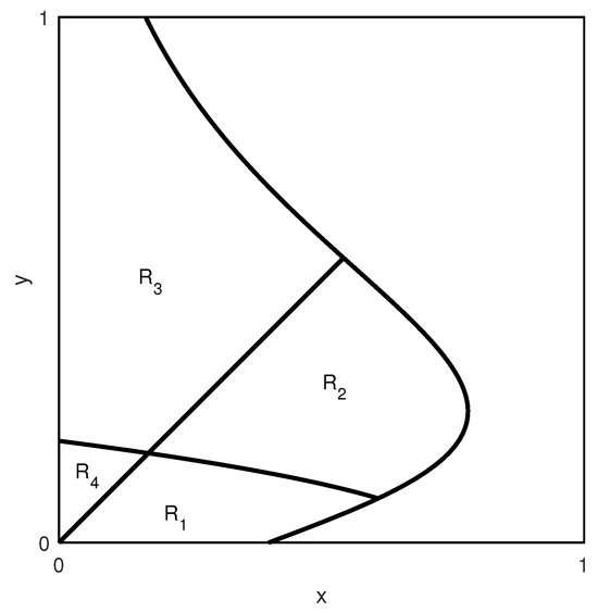
Figure 4. The figure depicts a generic representation of the regions $R_i$ as determined by the isoclines and the curve $LC$. In the plot shown, the parameter values are $\alpha ={\displaystyle \frac{3}{4}}$, $\beta =20$, and $\sigma ={\displaystyle \frac{1}{2}}$, though Lemma 2, and the equations for the isoclines show that this plot is typical for all $\alpha \in (0,1)$, $\beta >0$, and $\sigma \in (0,1)$.

Theorem 4. 

Let $\alpha \in (0,1)$, $\beta >0$, and $\sigma \in (0,1)$. Then, the following relations hold:

1. 

$F\left(R_1\right)\subseteq I_1^{-}$,

2. 

$F\left(R_2\right)\subseteq I_2^{+}$,

3. 

$F\left(R_3\right)\subseteq I_1^{+}$,

4. 

$F\left(R_4\right)\subseteq I_2^{-}$.

Proof. 

We prove (1) and (2) as the other proofs are similar with reversed inequalities.

1.

Let $(x,y)\in R_1=I_1^{-}\cap I_2^{-}$, so that $0\le y\le x$ and $x+\beta y^2\le \alpha$. Then,

$$\begin{array}{cc}\hfill y(1-{\sigma }^2)& \le x(1-{\sigma }^2)\hfill \\ & \le x(e^{\alpha -x-\beta y^2}-{\sigma }^2)\hfill \\ & =f(x,y)-{\sigma }^{2}x,\hfill \end{array}$$

which after rearrangement yields $g(x,y)\le f(x,y)$. That is, $F_U(x,y)\in I_1^{-}$.

2.

First, note that if $0\le x_1\le x_2\le 1$, then $f(x_1,y)\le f(x_2,y)$ and $g(x_1,y)\le g(x_2,y)$. Since the graph of $I_2$ is decreasing, it suffices to prove the claim on the left boundary of $I_1^{-}\cap I_2^{+}$. That is, it suffices to prove the result for $(x,y)$ where $x\ge x^{\ast }$ and either $x=y$ or $x+\beta y^2=\alpha$.

In the first case,

$$\begin{array}{cc}\hfill f(x,y)+\beta g{(x,y)}^2& =f(x,x)+\beta g{(x,x)}^2\hfill \\ & =x{e}^{\alpha -x-\beta x^2}+\beta x^2\hfill \end{array}$$

Since the derivative of $x{e}^{\alpha -x-\beta x^2}+\beta x^2$ is $(1-x)e^{\alpha -x-\beta x^2}+2\beta x(1-x{e}^{\alpha -x-\beta x^2})$, it is a strictly increasing function of x for $x\ge x^{\ast }$, and we have that

$$\begin{array}{cc}\hfill x{e}^{\alpha -x-\beta x^2}+\beta x^2& \ge x^{\ast }{e}^{\alpha -x^{\ast }-\beta {\left(x^{\ast }\right)}^2}+\beta {\left(x^{\ast }\right)}^2\hfill \\ & =x^{\ast }+\beta {\left(x^{\ast }\right)}^2\hfill \\ & =\alpha .\hfill \end{array}$$

In the second case, $f(x,y)=x$ and $g(x,y)\ge y$, so

$$\begin{array}{cc}\hfill f(x,y)+\beta g{(x,y)}^2& \ge x+\beta y^2\hfill \\ & \ge \alpha .\hfill \end{array}$$

□

Thus, not only do points in U proceed counterclockwise around $(x^{\ast },x^{\ast })$ under the mapping $F_U$, but in each loop around $(x^{\ast },x^{\ast })$ they cannot skip any of the $R_i$ in their itinerary. Consequently, we have the following corollary.

Corollary 1. 

Let $\alpha \in (0,1)$, $\beta >0$, and $\sigma \in (0,1)$. Then, $F_U$ has no points with minimal period 2 or 3.

Now, we turn to the stability of the two fixed points and their bifurcations.

Theorem 5. 

The origin is always a saddle point. The interior fixed point $(x^{\ast },x^{\ast })$ is locally asymptotically stable if and only if

$${\displaystyle \frac{{\sigma }^2(2\alpha -1)}{1+{\sigma }^2}}<x^{\ast }.$$

Proof. 

We use a Jacobian matrix. We calculate

$$J(0,0)=\left[\begin{array}{cc}{e}^{\alpha }& 0\\ {\sigma }^2& 1-{\sigma }^2\end{array}\right]$$

which has eigenvalues $e^{\alpha }>1$ and $1-{\sigma }^2\in (0,1)$, from which it follows that the origin is a saddle point. For the interior fixed point, we have

$$J(x^{\ast },x^{\ast })=\left[\begin{array}{cc}1-x^{\ast }& -2\beta {\left(x^{\ast }\right)}^2\\ {\sigma }^2& 1-{\sigma }^2\end{array}\right].$$

Using $x^{\ast }-\alpha =-\beta {\left(x^{\ast }\right)}^2$, we may also express this as

$$J(x^{\ast },x^{\ast })=\left[\begin{array}{cc}1-x^{\ast }& 2x^{\ast }-2\alpha \\ {\sigma }^2& 1-{\sigma }^2\end{array}\right].$$

From the Jury conditions [42], a necessary and sufficient criteria for local asymptotic stability of a fixed point is given by

$$\left|\mathrm{Tr}\right(J(x^{\ast },x^{\ast })|<det\left(J(x^{\ast },x^{\ast })\right)+1<2.$$

We claim that the first of these inequalities is always satisfied. Indeed, for the parameter values given, the trace is always positive since $x^{\ast }<\alpha <1$, so to verify the first inequality we simply observe that the stated inequality is equivalent to

$$2-x^{\ast }-{\sigma }^2<2-x^{\ast }-{\sigma }^2+x^{\ast }{\sigma }^2+2\beta {\left(x^{\ast }\right)}^2{\sigma }^2$$

which is equivalent to the true statement

$$0<x^{\ast }{\sigma }^2+2\beta {\left(x^{\ast }\right)}^2{\sigma }^2.$$

Using the second expression for $J(x^{\ast },x^{\ast })$, the second inequality requires that

$$1-x^{\ast }-{\sigma }^2+x^{\ast }{\sigma }^2-2x^{\ast }{\sigma }^2+2\alpha {\sigma }^2<1.$$

Rearranging, this is equivalent to

$$-{\sigma }^2+2\alpha {\sigma }^2<x^{\ast }+x^{\ast }{\sigma }^2.$$

Isolating the $x^{\ast }$ term yields

$${\displaystyle \frac{(2\alpha -1){\sigma }^2}{1+{\sigma }^2}}<x^{\ast }$$

as claimed. □

Example 2. 

Let $\alpha ={\displaystyle \frac{3}{4}}$ and $\sigma ={\displaystyle \frac{1}{2}}$. Then, $x^{\ast }={\displaystyle \frac{3}{2+2\sqrt{1+3\beta }}}$. From Theorem 5, $x^{\ast }$ is stable if and only if ${\displaystyle \frac{1}{10}}<x^{\ast }$. Solving ${\displaystyle \frac{1}{10}}<{\displaystyle \frac{3}{2+2\sqrt{1+3\beta }}}$ yields $\beta >65$, so that the fixed point loses stability at $\beta =65$. Indeed, at this value, we have $x^{\ast }={\displaystyle \frac{1}{10}}$ and

$$J\left({\displaystyle \frac{1}{10}},{\displaystyle \frac{1}{10}}\right)=\left[\begin{array}{cc}9/10& -13/10\\ 1/4& 3/4\end{array}\right].$$

The characteristic polynomial is given by $det\left(J\left(1/10,1/10\right)-\lambda \right)=0$ which yields

$${\lambda }^2-{\displaystyle \frac{33}{20}}\lambda +1=0.$$

The solutions to this quadratic yields the eigenvalues $\lambda ={\displaystyle \frac{33}{40}}\pm i{\displaystyle \frac{\sqrt{511}}{40}}$. A calculation shows that $\left|\lambda \right|=1$ for both eigenvalues so that the fixed point loses stability as β passes through 65.

Corollary 2. 

For $\sigma \in (0,1)$ and $0<\alpha \le {\displaystyle \frac{1}{2}}$, the fixed point $(x^{\ast },x^{\ast })$ is locally asymptotically stable for all $\beta >0$.

Proof. 

The bound

$${\displaystyle \frac{{\sigma }^2(2\alpha -1)}{1+{\sigma }^2}}<x^{\ast }$$

is trivially satisfied since $x^{\ast }>0$ and the left-hand side cannot be positive. □

Corollary 3. 

Let $\alpha \in ({\displaystyle \frac{1}{2}},1)$ and $\sigma \in (0,1)$. Then, the fixed point $(x^{\ast },x^{\ast })$ is locally asymptotically stable if and only if

$$\beta <{\displaystyle \frac{1}{4\alpha }}{\left({\displaystyle \frac{2\alpha +{\sigma }^2}{{\sigma }^2(2\alpha -1)}}\right)}^2-{\displaystyle \frac{1}{4\alpha }}.$$

Proof. 

The fixed point is locally asymptotically stable if and only if

$${\displaystyle \frac{{\sigma }^2(2\alpha -1)}{1+{\sigma }^2}}<{\displaystyle \frac{2\alpha }{1+\sqrt{1+4\alpha \beta }}}.$$

Since $\alpha >{\displaystyle \frac{1}{2}}$, the given inequality is equivalent to

$$\sqrt{1+4\alpha \beta }<{\displaystyle \frac{2\alpha +2\alpha {\sigma }^2}{{\sigma }^2(2\alpha -1)}}-1={\displaystyle \frac{2\alpha +{\sigma }^2}{{\sigma }^2(2\alpha -1)}}.$$

Squaring both sides and isolating $\beta$ gives the desired inequality. □

For fixed $\alpha \in ({\displaystyle \frac{1}{2}},1)$ and $\sigma \in (0,1)$, the mapping undergoes a bifurcation at the critical value $\beta ={\displaystyle \frac{1}{4\alpha }}{\left({\displaystyle \frac{2\alpha +{\sigma }^2}{{\sigma }^2(2\alpha -1)}}\right)}^2-{\displaystyle \frac{1}{4\alpha }}$. We recall that for smooth maps varying with a parameter, there are three types of bifurcations at a fixed point, depending on how the fixed point loses stability as the parameter changes. A fold bifurcation occurs when one of the eigenvalues of the Jacobian matrix becomes 1, while a period doubling bifurcation occurs when one of the eigenvalues of the Jacobian matrix becomes $-1$. A third type, Neimark–Sacker bifurcation, occurs when a pair of complex eigenvalues both have magnitude 1, such as in Example 2. For a comprehensive review of bifurcations, see [43]. We will prove momentarily that in Model (3), the fixed point $(x^{\ast },x^{\ast })$ has a Neimark–Sacker bifurcation at $\beta ={\displaystyle \frac{1}{4\alpha }}{\left({\displaystyle \frac{2\alpha +{\sigma }^2}{{\sigma }^2(2\alpha -1)}}\right)}^2-{\displaystyle \frac{1}{4\alpha }}$, if $\alpha \in ({\displaystyle \frac{1}{2}},1)$ and $\sigma \in (0,1)$, but does not undergo a fold (saddle node) bifurcation or flip (period doubling) bifurcation.

Proposition 2. 

For Model (3), let $\alpha \in (0,1)$ and $\sigma \in (0,1)$. Then, the fixed point $(x^{\ast },x^{\ast })$ does not undergo a flip or fold bifurcation at any $\beta >0$.

Proof. 

Fix $\alpha \in (0,1)$ and $\sigma \in (0,1)$. Let $x^{\ast }\left(\beta \right)={\displaystyle \frac{2\alpha }{1+\sqrt{1+4\alpha \beta }}}$. For brevity, let $T\left(\beta \right)=\mathrm{Tr}\left(J(x^{\ast },x^{\ast })\right)$ and $D\left(\beta \right)=det\left(J(x^{\ast },x^{\ast })\right)$.

The characteristic equation of $J(x^{\ast },x^{\ast })$ is given by ${\lambda }^2-T\left(\beta \right)\lambda +D\left(\beta \right)=0$. Thus, the eigenvalues ${\lambda }_{\pm }\left(\beta \right)$ of $J(x^{\ast },x^{\ast })$ are given by

$${\lambda }_{\pm }\left(\beta \right)={\displaystyle \frac{T\left(\beta \right)}{2}}\pm \sqrt{{\displaystyle \frac{T{\left(\beta \right)}^2}{4}}-D\left(\beta \right)}.$$

To have a fold bifurcation, we would need $\sqrt{{\displaystyle \frac{T{\left(\beta \right)}^2}{4}}-D\left(\beta \right)}$ to be real and for

$${\displaystyle \frac{T{\left(\beta \right)}^2}{4}}-D\left(\beta \right)={\left({\displaystyle \frac{T\left(\beta \right)}{2}}-1\right)}^2$$

or equivalently for

$$T\left(\beta \right)=D\left(\beta \right)+1.$$

Likewise, for a flip bifurcation we would need $\sqrt{{\displaystyle \frac{T{\left(\beta \right)}^2}{4}}-D\left(\beta \right)}$ to be real and for

$${\displaystyle \frac{T{\left(\beta \right)}^2}{4}}-D\left(\beta \right)={\left({\displaystyle \frac{T\left(\beta \right)}{2}}+1\right)}^2$$

or equivalently for

$$-T\left(\beta \right)=D\left(\beta \right)+1.$$

However, in the proof of Theorem 5, we proved that $\left|T\right(\beta \left)\right|<D\left(\beta \right)+1$, so we cannot have a fold or flip bifurcation. □

Lemma 3. 

For Model (3), let $\alpha \in ({\displaystyle \frac{1}{2}},1)$ and $\sigma \in (0,1)$. Let ${\beta }^{\ast }={\displaystyle \frac{1}{4\alpha }}{\left({\displaystyle \frac{2\alpha +{\sigma }^2}{{\sigma }^2(2\alpha -1)}}\right)}^2-{\displaystyle \frac{1}{4\alpha }}$ and let $\left(x^{\ast }\left({\beta }^{\ast }\right),x^{\ast }\left({\beta }^{\ast }\right)\right)$ denote the interior fixed point. Then, the eigenvalues ${\lambda }_{\pm }$ of $J(x^{\ast },x^{\ast })$ satisfy $|{\lambda }_{\pm }|=1$.

Proof. 

Fix $\alpha \in ({\displaystyle \frac{1}{2}},1)$ and $\sigma \in (0,1)$. Let ${\beta }^{\ast }={\displaystyle \frac{1}{4\alpha }}{\left({\displaystyle \frac{2\alpha +{\sigma }^2}{{\sigma }^2(2\alpha -1)}}\right)}^2-{\displaystyle \frac{1}{4\alpha }}$ and let $x^{\ast }\left(\beta \right)={\displaystyle \frac{2\alpha }{1+\sqrt{1+4\alpha \beta }}}$. As in the proof of Proposition 2, let $T\left(\beta \right)=\mathrm{Tr}(J(x^{\ast },x^{\ast })$ and $D\left(\beta \right)=det(J(x^{\ast },x^{\ast })$. The eigenvalues ${\lambda }_{\pm }\left(\beta \right)$ of $J(x^{\ast },x^{\ast })$ are given by

$${\lambda }_{\pm }\left(\beta \right)={\displaystyle \frac{T\left(\beta \right)}{2}}\pm \sqrt{{\displaystyle \frac{T{\left(\beta \right)}^2}{4}}-D\left(\beta \right)}.$$

Since $x^{\ast }<\alpha <1$, we have $0<T\left(\beta \right)<2$, and consequently we have ${\displaystyle \frac{T{\left(\beta \right)}^2}{4}}<1$. We note $D\left({\beta }^{\ast }\right)=1$, so in a neighborhood of ${\beta }^{\ast }$ the eigenvalues ${\lambda }_{\pm }\left(\beta \right)$ are complex and are given by

$${\lambda }_{\pm }\left(\beta \right)={\displaystyle \frac{T\left(\beta \right)}{2}}\pm i\sqrt{D\left(\beta \right)-{\displaystyle \frac{T{\left(\beta \right)}^2}{4}}}$$

with $|{\lambda }_{\pm }\left(\beta \right)|={\displaystyle \frac{T{\left(\beta \right)}^2}{4}}+D\left(\beta \right)-{\displaystyle \frac{T{\left(\beta \right)}^2}{4}}=D\left(\beta \right)$. Thus, both eigenvalues have magnitude 1 at $\beta ={\beta }^{\ast }$. □

As $\beta$ passes through the bifurcation value ${\beta }^{\ast }$, the fixed point loses stability, and Lemma 3 shows the possibility of a Neimark–Sacker bifurcation. One of the main features of Neimark–Sacker bifurcations is the introduction of closed invariant curves. In a supercritical Neimark–Sacker bifurcation, the fixed point loses stability and stable invariant curves appear, while in a subcritical Neimark–Sacker bifurcation, there are unstable closed invariant curves that vanish at the same time the fixed point loses stability. Whether such a bifurcation is supercritical or subcritical can be determined by converting the map to the Neimark–Sacker normal form. However, this normal form changes depending on whether two nondegeneracy conditions are satisfied. The main theorem for the generic case is given below.

Theorem 6 

([43]). Suppose a two-dimensional discrete-time system

$$\mathbf{x}\mapsto F(\mathbf{x},\beta ),\mathbf{x}\in {\mathbb{R}}^2,\beta \in \mathbb{R}$$

with smooth F has a fixed point ${\mathbf{x}}^{\ast }\left(\beta \right)$, where $DF\left({\mathbf{x}}^{\ast }\right)$ has eigenvalues

$${\lambda }_{\pm }\left(\beta \right)=r\left(\beta \right)e^{\pm i\theta \left(\beta \right)},$$

where $r\left({\beta }^{\ast }\right)=1$ and $\theta \left({\beta }^{\ast }\right)={\theta }_0$. Let the following conditions be satisfied:

• (C.1) $r^{\prime }\left({\beta }^{\ast }\right)\ne 0$
• (C.2) $e^{ik{\theta }_0}\ne 1$ for $k=1,2,3,4$

Then, by the introduction of a complex variable z and a parameter transformation $\gamma =r\left(\beta \right)-1$, the mapping $\mathbf{x}\mapsto F(\mathbf{x},\beta )$ can be transformed into the Poincare normal form

$$z\mapsto e^{i\theta \left(\gamma \right)}(1+\gamma +\left(d\left(\gamma \right)+ib\left(\gamma \right)\right){\left|z\right|}^2{)z+O(\left|z\right|}^4)$$

with parameter γ. If $d\left(0\right)<0$, then the bifurcation is supercritical, and if $d\left(0\right)>0$, then the bifurcation is subcritical.

Lemma 4. 

For Model (3), conditions (C.1) and (C.2) in Theorem 6 are satisfied for $\alpha \in ({\displaystyle \frac{1}{2}},1)$ and $\sigma \in (0,1)$.

Proof. 

Fix $\alpha \in ({\displaystyle \frac{1}{2}},1)$ and $\sigma \in (0,1)$, and let $x^{\ast }\left(\beta \right)={\displaystyle \frac{2\alpha }{1+\sqrt{1+4\alpha \beta }}}$ denote the fixed point and ${\beta }^{\ast }={\displaystyle \frac{1}{4\alpha }}{\left({\displaystyle \frac{2\alpha +{\sigma }^2}{{\sigma }^2(2\alpha -1)}}\right)}^2-{\displaystyle \frac{1}{4\alpha }}$ denote the bifurcation value. Note that ${\left(x^{\ast }\right)}^{\prime }\left(\beta \right)<0$ and that

$$\begin{array}{cc}\hfill r\left(\beta \right)& =|{\lambda }_{\pm }\left(\beta \right)|\hfill \\ & =D\left(\beta \right)\hfill \\ & =(1-x^{\ast })(1-{\sigma }^2)-2x^{\ast }{\sigma }^2+2\alpha {\sigma }^2.\hfill \end{array}$$

It then follows that

$$\begin{array}{cc}\hfill r^{\prime }\left(\beta \right)& ={\left(x^{\ast }\right)}^{\prime }\left(\beta \right)({\sigma }^2-3)\hfill \\ & >0.\hfill \end{array}$$

In particular, $r^{\prime }\left({\beta }^{\ast }\right)>0$ so that condition (C.1) is satisfied.

Since

$$e^{ik{\theta }_0}={\lambda }_{+}^k\left({\beta }^{\ast }\right)={\left({\displaystyle \frac{T\left({\beta }^{\ast }\right)}{2}}\pm i\sqrt{1-{\displaystyle \frac{T{\left({\beta }^{\ast }\right)}^2}{4}}}\right)}^k,$$

we only have $e^{ik{\theta }_0}=1$ for $k\in \{1,2,3,4\}$ if $T\left({\beta }^{\ast }\right)\in \{-2,-1,0,2\}$, which is not the case as $T\left({\beta }^{\ast }\right)\in (0,2)$. Thus, condition (C.2) is satisfied. □

Lemmas 3 and 4 are sufficient to establish the following proposition.

Proposition 3. 

Let $\alpha \in ({\displaystyle \frac{1}{2}},1)$ and $\sigma \in (0,1)$. Then, the fixed point $(x^{\ast },x^{\ast })$ undergoes a Neimark–Sacker bifurcation at $\beta ={\displaystyle \frac{1}{4\alpha }}{\left({\displaystyle \frac{2\alpha +{\sigma }^2}{{\sigma }^2(2\alpha -1)}}\right)}^2-{\displaystyle \frac{1}{4\alpha }}$.

A prototype of the stability region in the parameter space is shown in Figure 5. For $\alpha ,\sigma$, and $\beta$ within the shaded region, the interior fixed point $(x^{\ast },x^{\ast })$ is locally asymptotically stable, corresponding to the region referenced in the conditions of Theorem 5. The conditions in Corollary 2 define the region on the left side of the concave portion such that $\alpha \le {\displaystyle \frac{1}{2}}$, while the conditions in Corollary 3 define the region below the concave portion such that $\alpha >{\displaystyle \frac{1}{2}}$. The Neimark–Sacker bifurcation mentioned in Proposition 3 occurs precisely on the surface of the concave part.

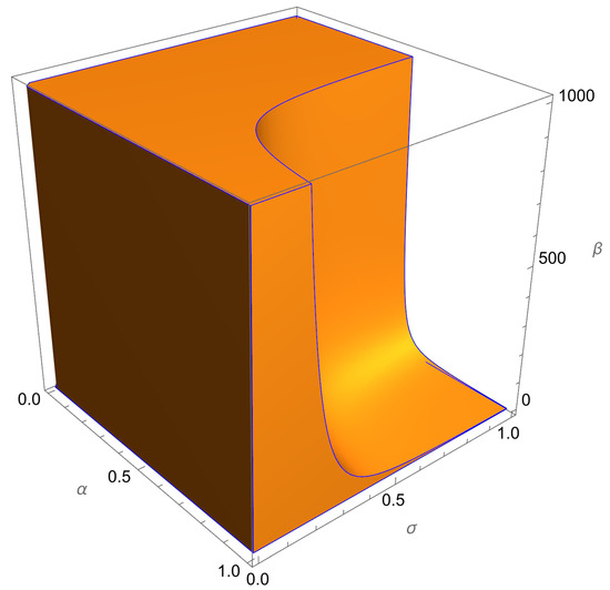
Figure 5. A prototype of the stability region in the parameter space of the interior fixed point $(x^{\ast },x^{\ast })$ of Model (3).

While we have established the existence of a Neimark–Sacker bifurcation, the computations thus far have not yet shown if it is supercritical or subcritical. In principle, one can calculate the coefficient $d\left(0\right)$ from Theorem 6, but the calculation for Model (3) is lengthy and impractical, as it does not allow one to determine the sign of $d\left(0\right)$ for general parameter values (see Appendix A), due to the size of the coefficients involved. Instead, we will present a geometric argument using stable and unstable manifolds in the next section.

5. Stable and Unstable Manifolds

For a fixed point $\mathbf{p}$ of an invertible mapping $F:X\to X$, we denote the stable manifold of $\mathbf{p}$ by

$$W^s\left(\mathbf{p}\right)=\{x\in X:\underset{n\to \infty }{lim}{F}^n\left(x\right)=\mathbf{p}\}$$

and likewise its unstable manifold by

$$W^s\left(\mathbf{p}\right)=\{x\in X:\underset{n\to \infty }{lim}{F}^{-n}\left(x\right)=\mathbf{p}\}.$$

For the mapping $F_U$, the stable manifold of the origin is the portion of the y-axis that lies in U, that is, $W^s(0,0)=\{(x,y)\in U:x=0\}$.

Some numerically computed images of the unstable manifold at the origin are shown in Figure 6. We will now proceed to show these plots are typical.

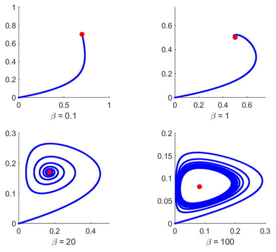
Figure 6. Numerically computed the unstable manifolds of the origin for $\alpha ={\displaystyle \frac{3}{4}}$ and $\sigma ={\displaystyle \frac{1}{2}}$. The $\beta$ values in the four plots are $0.1$, 1, 20, and 100, respectively. The fixed point $(x^{\ast },x^{\ast })$ for $\alpha ={\displaystyle \frac{3}{4}}$ and $\sigma ={\displaystyle \frac{1}{2}}$ is locally asymptotically stable for $\beta <65$. In the first three images, $(x^{\ast },x^{\ast })$ is locally asymptotically stable and the unstable manifold $W^u(0,0)$ is asymptotic to the fixed point $(x^{\ast },x^{\ast })$. For small $\beta$, it converges directly to it, while for larger $\beta$ it spirals into it. In the last image, these spirals converge to an invariant curve instead of to the unstable fixed point.

In $J(0,0)$, the eigenvector $\left[\begin{array}{c}{\sigma }^2+(e^{\alpha }-1)\\ {\sigma }^2\end{array}\right]$ corresponds to the unstable direction in the linearized map with eigenvalue $e^{\alpha }$. Since $W^u(0,0)$ lies tangent to this eigenvector, $W^u(0,0)$ is initially in $R_1$. We also recall the cycling nature of the $R_i$, the direction of the mapping in each $R_i$, and that the manifold cannot self-intersect. These facts ensure the argument of $W^u(0,0)$ is strictly increasing when viewed as centered at $(x^{\ast },x^{\ast })$.

If the curve remains in $R_1$, then it must monotonically approach $(x^{\ast },x^{\ast })$. Otherwise, it must eventually intersect $I_2$ so that it enters $R_2$. Again, if it remains in $R_2$, then it must monotonically approach $(x^{\ast },x^{\ast })$, otherwise it must intersect $I_1$. Eventually, if it does not stay in some $R_i$, it will intersect the isoclines an infinite number of times as it spirals counterclockwise. Viewing $(x^{\ast },x^{\ast })$ as the center and looking at polar coordinates $(r,{\theta }^{\ast })$, we can look at the return map that gives the radius r from $(x^{\ast },x^{\ast })$ generated by intersections with any fixed $\theta$ value. Since the manifold does not self intersect, these return maps are strictly decreasing. As they are also bounded, we conclude the following theorem.

Theorem 7. 

Let $\alpha \in (0,1)$, $\beta >0$, and $\sigma \in (0,1)$. Then, the unstable manifold $W^u(0,0)$ is asymptotic to either the fixed point $(x^{\ast },x^{\ast })$ or a closed curve that encloses $(x^{\ast },x^{\ast })$.

In Figure 6, we illustrate the concept underlying Theorem 7. As is clearly seen in the presented four examples, all the orbits behave in a counterclockwise manner, either converging to the fixed point when the absolute values of both eigenvalues are less than one or orbiting around the fixed point when both eigenvalues exceed absolute value 1. This is precisely the main idea behind the proof of Theorem 7.

Let us now fix $\alpha$ and $\sigma$ and see how the unstable manifold evolves as $\beta$ increases. First, we prove the following lemma.

Lemma 5. 

Let $\alpha ,\sigma \in (0,1)$. Let $p\left(\beta \right)$ denote the discriminant of the characteristic polynomial of $J\left(x^{\ast },x^{\ast }\right)$. Then $p^{\prime }\left(\beta \right)<0$.

Proof. 

Recall that we have $p\left(\beta \right)={\displaystyle \frac{T{\left(\beta \right)}^2}{4}}-D\left(\beta \right)$, where

$$\begin{array}{cc}\hfill D\left(\beta \right)& =det(J(x^{\ast },x^{\ast })\hfill \\ & =\left|\begin{array}{cc}1-x^{\ast }& 2x^{\ast }-2\alpha \\ {\sigma }^2& 1-{\sigma }^2\end{array}\right|\hfill \\ & =1-x^{\ast }-{\sigma }^2+{\sigma }^2{x}^{\ast }-2x^{\ast }{\sigma }^2+2\alpha {\sigma }^2\hfill \\ & =(1-{\sigma }^2+2{\sigma }^2\alpha )+x^{\ast }(-{\sigma }^2-1),\hfill \end{array}$$

$$\begin{array}{cc}\hfill T\left(\beta \right)& =\mathrm{Trace}\left(J(x^{\ast },x^{\ast })\right)\hfill \\ & =2-x^{\ast }-{\sigma }^2\hfill \end{array}$$

and

$$x^{\ast }={\displaystyle \frac{2\alpha }{1+\sqrt{1+4\alpha \beta }}}.$$

Note also that ${\displaystyle \frac{\partial x^{\ast }}{\partial \beta }}<0$.

Then,

$$\begin{array}{cc}\hfill p^{\prime }\left(\beta \right)& =-{\displaystyle \frac{1}{2}}T\left(\beta \right){\displaystyle \frac{\partial x^{\ast }}{\partial \beta }}-{\displaystyle \frac{\partial x^{\ast }}{\partial \beta }}(-{\sigma }^2-1)\hfill \\ & ={\displaystyle \frac{\partial x^{\ast }}{\partial \beta }}\left(-1+{\displaystyle \frac{1}{2}}{x}^{\ast }+{\displaystyle \frac{1}{2}}{\sigma }^2+{\sigma }^2+1\right)\hfill \\ & ={\displaystyle \frac{\partial x^{\ast }}{\partial \beta }}\left({\displaystyle \frac{1}{2}}{x}^{\ast }+{\displaystyle \frac{3}{2}}{\sigma }^2\right)\hfill \\ & <0.\hfill \end{array}$$

□

Initially, when $\beta =0$, it is straightforward to prove the set $R_1$ is forward invariant, so that the unstable manifold $W^u(0,0)$ forms a heteroclinic connection between the origin and $(x^{\ast },x^{\ast })$. In this case, $x^{\ast }=\alpha$, and the eigenvalues of $J(x^{\ast },x^{\ast })$ are $1-\alpha$ and $1-{\sigma }^2$, i.e., $p\left(0\right)>0$. The heteroclinic connection for $\beta =0$ persists under perturbations of $\beta$ and is tangent to one of the eigenvectors at $(x^{\ast },x^{\ast })$. This idea is illustrated in Figure 7. In this example, the tangency is clearly observed. Let us examine some properties of these eigenvectors in more detail.

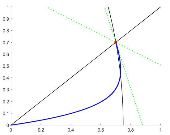
Figure 7. Numerically computed unstable manifold $W^u(0,0)$ for $\alpha ={\displaystyle \frac{3}{4}}$, $\beta ={\displaystyle \frac{1}{10}}$, and $\sigma ={\displaystyle \frac{1}{2}}$, along with lines parallel to the eigenvectors at $(x^{\ast },x^{\ast })$ (shown as dotted lines). The isoclines are also shown.

Lemma 6. 

Let $\alpha ,\sigma \in (0,1)$. Let β be such that the eigenvalues of $J(x^{\ast },x^{\ast })$ are real. Then, any eigenvalue λ of $J(x^{\ast },x^{\ast })$ satisfies $0<\lambda <1-{\sigma }^2$.

Proof. 

Since $\lambda$ is an eigenvalue of $J(x^{\ast },x^{\ast })$, then

$$\left[\begin{array}{cc}1-x^{\ast }-\lambda & 2x^{\ast }-2\alpha \\ {\sigma }^2& 1-{\sigma }^2-\lambda \end{array}\right]$$

has vanishing determinant. Since ${\sigma }^2>0$ and $2x^{\ast }-2\alpha <0$, the product

$$(1-x^{\ast }-\lambda )(1-{\sigma }^2-\lambda )$$

must be negative. Since $x^{\ast }<\alpha <1$, if $\lambda \le 0$, then both terms are positive. If $\lambda \ge 1-{\sigma }^2$, then both terms are negative or zero. This implies $0<\lambda <1-{\sigma }^2$. □

If $\lambda$ is a real eigenvalue of $J(x^{\ast },x^{\ast })$, then the line through $(x^{\ast },x^{\ast })$ that is parallel to the corresponding eigenvector has a slope of ${\displaystyle \frac{-{\sigma }^2}{1-{\sigma }^2-\lambda }}$. From the previous lemma, this slope is always negative. The larger of the two eigenvalues, given by ${\lambda }^{+}={\displaystyle \frac{T\left(\beta \right)}{2}}+\sqrt{{\displaystyle \frac{T{\left(\beta \right)}^2}{4}}-D\left(\beta \right)}$, corresponds to the line with a steeper slope. It is this line that $W^u(0,0)$ is asymptotic to.

A calculation shows

$$\begin{array}{cc}\hfill \underset{\beta \to \infty }{lim}p\left(\beta \right)& ={\displaystyle \frac{{(2-{\sigma }^2)}^2}{4}}-1+{\sigma }^2-2{\sigma }^2\alpha \hfill \\ & ={\displaystyle \frac{{\sigma }^2}{4}}({\sigma }^2-8\alpha ).\hfill \end{array}$$

If $\alpha \le {\displaystyle \frac{{\sigma }^2}{8}}$, then by continuity the eigenvalues of $J(x^{\ast },x^{\ast })$ remain real for all $\beta$. For $\alpha >{\displaystyle \frac{{\sigma }^2}{8}}$, eigenvalues transition at a critical value $\overline{\beta }$ from real to complex. At such values, the curve $W^u(0,0)$ transitions from directly looping into $(x^{\ast },x^{\ast })$ and instead starts an infinite spiral, intersecting the isoclines an infinite number of times.

If $W^u(0,0)$ is asymptotic to a closed curve, then that curve is necessarily stable. Consequently, the curve cannot be an unstable curve that emerged from a subcritical Neimark–Sacker bifurcation. For $\overline{\beta }<\beta <{\beta }^{\ast }$, this spiral approaches $(x^{\ast },x^{\ast })$ and the heteroclinic orbit is maintained. At ${\beta }^{\ast }$, the heteroclinic orbit breaks as a supercritical Neimark–Sacker bifurcation occurs, and a stable closed curve bifurcates from the fixed point for $\beta >{\beta }^{\ast }$.

Example 3. 

Let $\alpha ={\displaystyle \frac{3}{4}}$ and $\sigma ={\displaystyle \frac{1}{2}}$, so that $x^{\ast }={\displaystyle \frac{3}{2+2\sqrt{1+3\beta }}}$. We have

$$T\left(\beta \right)={\displaystyle \frac{7}{4}}-x^{\ast }$$

and

$$D\left(\beta \right)={\displaystyle \frac{9}{8}}-{\displaystyle \frac{5}{4}}{x}^{\ast }.$$

The eigenvalues of $J(x^{\ast },x^{\ast })$ are real provided

$${\displaystyle \frac{T{\left(\beta \right)}^2}{4}}-D\left(\beta \right)>0$$

which yields

$${\displaystyle \frac{1}{4}}{\left(x^{\ast }\right)}^2+{\displaystyle \frac{3}{8}}{x}^{\ast }-{\displaystyle \frac{23}{64}}>0$$

which for positive $x^{\ast }$ implies that the eigenvalues are real if $x^{\ast }>\sqrt{2}-{\displaystyle \frac{3}{4}}$. Solving

$${\displaystyle \frac{3}{2+2\sqrt{1+3\beta }}}>\sqrt{2}-{\displaystyle \frac{3}{4}}$$

for positive β yields

$$\beta <{\displaystyle \frac{216}{529}}-{\displaystyle \frac{80}{529}}\sqrt{2}.$$

Thus, $\overline{\beta }={\displaystyle \frac{216}{529}}-{\displaystyle \frac{80}{529}}\sqrt{2}$. Since ${\beta }^{\ast }=65$ (see Example 2), the dynamics for $\alpha ={\displaystyle \frac{3}{4}}$ and $\sigma ={\displaystyle \frac{1}{2}}$ may be described as follows. For $0<\beta <{\displaystyle \frac{216}{529}}-{\displaystyle \frac{80}{529}}\sqrt{2}$, the unstable manifold $W^u(0,0)$ is tangent to the real eigenvector and convergence to the fixed point is guaranteed. For ${\displaystyle \frac{216}{529}}-{\displaystyle \frac{80}{529}}\sqrt{2}<\beta <65$, the eigenvalues are now complex, and the unstable manifold infinitely spirals around the fixed point, but still converges to it. For $\beta >65$, where the Neimark–Sacker bifurcation occurs, a new forward invariant closed curve appears and the unstable manifold spirals towards this curve instead. See also Figure 6.

In all cases, since $W^u(0,0)$ forms a barrier which points cannot cross, this unstable manifold dictates global behavior on $F_U$. In particular, in the absence of a closed invariant curve, the fixed point is globally asymptotically stable.

6. Conclusions

In this paper, we studied the local properties, the global properties, and the bifurcation of a nonlinear planar system of coupled difference equations consisting of the evolution of a species of Ricker type. By studying the model when the trait equation is coupled from the population dynamic equation, we were able to conclude that, under certain restrictions on the parameters, the model is forward invariant and globally attracting in a subset of the phase space, bounded by the coordinate axes, the horizontal line $y=1$, and a critical curve $LC$, which is the image under the mapping that rules the model where the Jacobian vanishes. We show that in this subset of the phase space, there are four regions where the orbits behave in a cyclic nature (counterclockwise direction) and converge towards the asymmetric unstable manifold of the origin, which will attract all the orbits.

Moreover, in this set, the model possesses two symmetric fixed points: the origin, which is always a saddle fixed point, and an interior fixed point that is locally asymptotically stable for certain values of the parameters. This non-trivial fixed point undergoes a Neimark–Sacker bifurcation for a critical parameter value, a phenomenon that does not occur in the original one-dimensional Ricker model. By using a geometric argument with the unstable manifold at the origin, we show that this bifurcation is supercritical, and thus a stable asymmetric closed curve bifurcates from the fixed point once we cross the critical value. Finally, in the absence of the referred closed invariant curve, the symmetric non-trivial fixed point is globally asymptotically stable.

We have utilized tools from both analytic and geometric approaches to achieve our goals. The analytic tools are similar to those existing in the literature for these types of models, including the relative position of critical curves using singularity theory, the dynamics of sets around the isoclines, and local stability using Jury’s conditions.

Typically, the study and classification of the Neimark–Sacker bifurcation are conducted using the normal forms of the equations. Nondegeneracy conditions are usually computed by taking certain derivatives, as explained in Section 4. However, in Model (3), we were unable to use $d\left(0\right)$ to classify the bifurcation, as is mentioned in the end of Section 4. Therefore, we employed a geometric argument, which, to the best of our knowledge, is the first time it has been used in this context. This geometric argument allowed us to demonstrate the global stability of the positive fixed point, meaning that every orbit of a point in the interior of the first quadrant will eventually converge to the fixed point. This is a central conclusion in real-world applications, particularly in ecology.

We should mention that the tools employed in this model are extendable to other discrete evolutionary models as well, such as the evolutionary Beverton–Holt model and the logistic model.

7. Future Work

In future work, we plan to study the dynamics of the model in seasonal environments, specifically focusing on how the discrete model behaves under periodic changes. This involves analyzing how the system’s behavior is influenced by parameters that fluctuate regularly, reflecting seasonal variations in the environment. In particular, we aim to understand how these periodic parameter changes affect the long-term dynamics of the model, i.e., the study of the model

$$\begin{array}{c}\hfill \left\{\begin{array}{c}{x}_{n+1}=x_n{e}^{{\alpha }_n-\beta y_n^2-x_n}\hfill \\ y_{n+1}=(1-{\sigma }^2)y_n+{\sigma }^2{x}_n\hfill \end{array}\right.,\end{array}$$

(4)

when the sequence of parameters ${\alpha }_n$ is $p$-periodic, i.e., ${\alpha }_{n+p}={\alpha }_n$ for all n and some integer $p>1$.

We believe that the orbits in the periodic model (4) will exhibit similar behavior, with counterclockwise dynamics around the periodic cycle in phase space. Furthermore, since it will be challenging to explicitly write the periodic solution, the geometric method developed for classifying the Neimark–Sacker bifurcation will be a useful tool. As observed in simulations, if the period of the cycle equals the period of the system, the same number of cycling orbits circulate counterclockwise around the periodic points. Moreover, when the eigenvalues of the Jacobian of the composition map, evaluated at the periodic orbit, have absolute values less than one, convergence can be observed. Thus, the geometric approach will be a valuable method for classifying the nature of the invariant manifolds and the dynamics around the isoclines.

Understanding these dynamics can provide insights into the long-term behavior and global stability of the population under study. In particular, it will be interesting to determine whether the periodic evolutionary model exhibits attenuation, resonance, or neither attenuation nor resonance, a phenomenon observed by R. Sacker [44] in the periodic one-dimensional Ricker model.

We also plan to use similar techniques to study a generalization of Model (3) for n competing species, resulting in a model with $2n$ equations. Our real challenge will be generalizing the geometric approach to higher dimensions, as it may become impossible to explicitly compute the fixed points after a certain number of species. Hence, a geometric approach will be crucial.

An interesting study would also investigate whether our tools are applicable to a model similar to Model (3) but with several traits in the canonical equation for evolution.

References

- Ricker, E. Stock and recruitment. J. Fish. Res. Board Can. 1954, 11, 559–623. [Google Scholar] [CrossRef]
- May, R.M.; Oster, G.F. Bifurcations and Dynamic Complexity in Simple Ecological Models. Am. Nat. 1976, 110, 573–599. [Google Scholar] [CrossRef]
- Costantino, R.F.; Desharnais, R.A.; Cushing, J.M.; Dennis, B. Chaotic Dynamics in an Insect Population. Science 1997, 275, 389–391. [Google Scholar] [CrossRef]
- Zimmer, C. Life After Chaos. Science 1999, 284, 83–86. [Google Scholar] [CrossRef]
- Ackleh, A.S.; Cushing, J.M.; Salceanu, P.L. On the dynamics of evolutionary competition models. Nat. Resour. Model. 2015, 28, 380–397. [Google Scholar] [CrossRef]
- Cushing, J.M. An evolutionary Beverton–Holt model. In Theory and Applications of Difference Equations and Discrete Dynamical Systems; Springer: Berlin/Heidelberg, Germany, 2014; Volume 102, pp. 127–141. [Google Scholar] [CrossRef]
- Cushing, J.M. Difference equations as models of evolutionary population dynamics. J. Biol. Dyn. 2019, 13, 103–127. [Google Scholar] [CrossRef]
- Cushing, J.M. A Darwinian Ricker equation. In Progress on Difference Equations and Discrete Dynamical Systems; Springer: Cham, Switzerland, 2020; Volume 341, pp. 231–243. [Google Scholar] [CrossRef]
- Cushing, J.M.; Stefanko, K. A Darwinian dynamic model for the evolution of post-reproduction survival. J. Biol. Syst. 2021, 29, 433–450. [Google Scholar] [CrossRef]
- Cushing, J.M. The evolutionary dynamics of a population model with a strong Allee effect. Math. Biosci. Eng. 2015, 12, 643–660. [Google Scholar] [CrossRef]
- Rael, R.C.; Vincent, T.L.; Cushing, J.M. Competitive outcomes changed by evolution. J. Biol. Dyn. 2011, 5, 227–252. [Google Scholar] [CrossRef]
- Darwin, C. The Origin of Species; Avenel Books: London, UK, 1859. [Google Scholar]
- Weibull, J.W. Evolutionary Game Theory; MIT Press: Cambridge, MA, USA, 1995. [Google Scholar]
- Vincent, T.L.; Brown, J.S. Evolutionary Game Theory, Natural Selection, and Darwinian Dynamics; Cambridge University Press: Cambridge, UK, 2005. [Google Scholar]
- Ch-Chaoui, M.; Mokni, K. A discrete evolutionary Beverton–Holt population model. Int. J. Dyn. Control 2023, 11, 1060–1075. [Google Scholar] [CrossRef]
- Mokni, K.; Ch-Chaoui, M. Asymptotic stability, bifurcation analysis and chaos control in a discrete evolutionary Ricker population model with immigration. In Advances in Discrete Dynamical Systems, Difference Equations and Applications; Springer: Cham, Switzerland, 2023; Volume 416, pp. 363–403. [Google Scholar] [CrossRef]
- Elaydi, S.; Kang, Y.; Luís, R. The effects of evolution on the stability of competing species. J. Biol. Dyn. 2022, 16, 816–839. [Google Scholar] [CrossRef] [PubMed]
- Mokni, K.; Elaydi, S.; Ch-Chaoui, M.; Eladdadi, A. Discrete evolutionary population models: A new approach. J. Biol. Dyn. 2020, 14, 454–478. [Google Scholar] [CrossRef]
- Elaydi, S.; Kang, Y.; Luís, R. Global asymptotic stability of evolutionary periodic Ricker competition models. J. Differ. Equ. Appl. 2024, 30, 1091–1116. [Google Scholar] [CrossRef]
- Rosenkranz, G. On global stability of discrete population models. Math. Biosci. 1983, 64, 227–231. [Google Scholar] [CrossRef]
- Cull, P. Stability in one-dimensional models. Sci. Math. Jpn. 2003, 58, 349–357. [Google Scholar]
- Singer, D. Stable orbits and bifurcation of maps of the interval. SIAM J. Appl. Math. 1978, 35, 260–267. [Google Scholar] [CrossRef]
- Smith, H.L. Planar competitive and cooperative difference equations. J. Differ. Equ. Appl. 1998, 3, 335–357. [Google Scholar] [CrossRef]
- Hirsch, M.W.; Smith, H. Monotone dynamical systems. In Handbook of Differential Equations: Ordinary Differential Equations; Elsevier: Amsterdam, The Netherlands, 2005; Volume II, pp. 239–357. [Google Scholar]
- Kulenović, M.R.S.; Moranjkić, S.; Nurkanović, M.; Nurkanović, Z. Global asymptotic stability and Naimark-Sacker bifurcation of certain mix monotone difference equation. Discret. Dyn. Nat. Soc. 2018, 2018, 7052935. [Google Scholar] [CrossRef]
- Balreira, E.C.; Elaydi, S.; Luís, R. Global stability of higher dimensional monotone maps. J. Differ. Equ. Appl. 2017, 23, 2037–2071. [Google Scholar] [CrossRef]
- Smith, H.L. Global stability for mixed monotone systems. J. Differ. Equ. Appl. 2008, 14, 1159–1164. [Google Scholar] [CrossRef]
- Whitney, H. On singularities of mappings of euclidean spaces. I. Mappings of the plane into the plane. Ann. Math. 1955, 62, 374–410. [Google Scholar] [CrossRef]
- Mira, C.; Gardini, L.; Barugola, A.; Cathala, J. Chaotic Dynamics in Two-Dimensional Noninvertible Maps; Nonlinear Sciences Series A; World Scientific: Singapore, 1996. [Google Scholar]
- Mira, C. Chaotic Dynamics; World Scientific: Singapore, 1987. [Google Scholar]
- Gardini, L. Some global bifurcations of two-dimensional endomorphisms by use of critical lines. Nonlinear Anal. 1992, 18, 361–399. [Google Scholar] [CrossRef]
- Cabral Balreira, E.; Elaydi, S.; Luís, R. Local stability implies global stability for the planar Ricker competition model. Discret. Contin. Dyn. Syst. Ser. B 2014, 19, 323–351. [Google Scholar] [CrossRef]
- Ryals, B.; Sacker, R.J. Global stability in the 2D Ricker equation. J. Differ. Equ. Appl. 2015, 21, 1068–1081. [Google Scholar] [CrossRef]
- Ryals, B.; Sacker, R.J. Global stability in the 2D Ricker equation revisited. Discret. Contin. Dyn. Syst. Ser. B 2017, 22, 585–604. [Google Scholar] [CrossRef][Green Version]
- Ryals, B. A note on a parameter bound for global stability in the 2D coupled Ricker equation. J. Differ. Equ. Appl. 2018, 24, 240–244. [Google Scholar] [CrossRef]
- Elaydi, S. Global dynamics of discrete dynamical systems and difference equations. In Difference Equations, Discrete Dynamical Systems And Applications; Springer: Cham, Switzerland, 2019; Volume 287, pp. 51–81. [Google Scholar] [CrossRef]
- Luís, R. Open Problems and Conjectures in the Evolutionary Periodic Ricker Competition Model. Axioms 2024, 13, 246. [Google Scholar] [CrossRef]
- Dercole, F.; Rinaldi, S. Analysis of Evolutionary Processes: The Adaptive Dynamics Approach and Its Applications; Princeton Series in Theoretical and Computational Biology; Princeton University Press: Princeton, NJ, USA, 2008. [Google Scholar]
- Lande, R. Natural selection and random genetic drift in phenotypic evolution. Evolution 1976, 30, 314–334. [Google Scholar] [CrossRef]
- Lande, R. A Quantitative Genetic Theory of Life History Evolution. Ecology 1982, 63, 607–615. [Google Scholar] [CrossRef]
- Abrams. Modelling the adaptive dynamics of traits involved in inter- and intraspecific interactions: An assessment of three methods. Ecol. Lett. 2001, 4, 166–175. [Google Scholar] [CrossRef]
- Jury, E. On the roots of a real polynomial inside the unit circle and a stability criterion for linear discrete systems. IFAC Proc. Vol. 1963, 1, 142–153. [Google Scholar] [CrossRef]
- Kuznetsov, Y.A. Elements of applied bifurcation theory. In Applied Mathematical Sciences, 4th ed.; Springer: Cham, Switzerland, 2023; Volume 112, pp. xxvi+703. [Google Scholar] [CrossRef]
- Sacker, R.J. A note on periodic Ricker maps. J. Differ. Equ. Appl. 2007, 13, 89–92. [Google Scholar] [CrossRef]
Disclaimer/Publisher’s Note: The statements, opinions and data contained in all publications are solely those of the individual author(s) and contributor(s) and not of MDPI and/or the editor(s). MDPI and/or the editor(s) disclaim responsibility for any injury to people or property resulting from any ideas, methods, instructions or products referred to in the content. |
© 2024 by the authors. Licensee MDPI, Basel, Switzerland. This article is an open access article distributed under the terms and conditions of the Creative Commons Attribution (CC BY) license (https://creativecommons.org/licenses/by/4.0/).