Advanced Bimodal Skew-Symmetric Distributions: Methodology and Application to Cancer Cell Protein Data

Abstract

This paper explores bimodal skew-symmetric distributions, a versatile family of distributions characterized by parameters that control asymmetry and kurtosis. These distributions encapsulate both symmetrical and well-known asymmetrical behaviors. A simulation study evaluates the model’s estimation accuracy, detailing the score function and the robustness of the observed information matrix, which is proven to be non-singular under specific conditions. We apply the bimodal skew-normal model to protein data from cancer cells, comparing its performance against four established distributions supported on the entire real line. Results indicate superior performance by the proposed model, underscoring its potential for enhancing analytical precision in biological research.

1. Introduction

The family of skew-symmetric distributions has been increasingly recognized for its flexibility and efficacy in modeling real-world data by transforming symmetric probability density functions (PDFs) with specific generators. This family is defined by the following PDF:

$$2f\left(z\right)G\left(w\right(z\left)\right),z\in \mathbb{R},$$

(1)

where f is a symmetric PDF centered at 0 and G is the cumulative distribution function (CDF) of a continuous random variable that is symmetric around 0. The function w is required to be odd and continuous, meaning $w(-z)+w\left(z\right)=0$.

This framework was initially developed by Azzalini [1,2], who introduced the skew-normal distribution by setting $f=G^{\prime }=\varphi$, the PDF of the standard normal distribution, and $w\left(z\right)=\lambda z$. This construction allows the skew-symmetric distribution to encapsulate both symmetric and skewed data through the parameter $\lambda$. Over time, various researchers (e.g., Gupta et al. [3], Ma and Genton [4], and Arellano-Valle et al. [5]) have expanded this model to include different forms of w, such as $w\left(z\right)={\lambda }_{1}z+{\lambda }_2{z}^3$ and $w\left(z\right)={\lambda }_{1}z/\sqrt{1+{\lambda }_2^2{z}^2}$, broadening its applicability within the skew-symmetric framework.

The general form (1) encompasses a wide range of submodels, from the symmetric density f (when $w\left(z\right)=0$) to the highly skewed half-f densities (as $w\left(z\right)\to \pm \infty$). These models can capture varying degrees of skewness in data, making them valuable in many statistical applications. For example, Pewsey [6] examined a subfamily where $w\left(z\right)=\lambda z$ for $\lambda \in \mathbb{R}$. However, the model $2{\eta }^{-1}f((x-\xi )/\eta )G(\lambda (x-\xi )/\eta )$, $x\in \mathbb{R}$, with location parameter $\xi$ and scale parameter $\eta$, encounters significant challenges in maximum likelihood estimation (MLE) when $G^{\prime }=f=\varphi$. Specifically, when $\lambda =0$, the expected information matrix becomes singular, complicating the estimation process. Pewsey also noted that the observed information matrix fails to have an inverse for the CDF G when $G^{″}\left(0\right)=g^{\prime }\left(0\right)=0$.

To address these challenges and further enhance the applicability of skew-symmetric distributions, we propose a novel w function that not only avoids the singularity issues at $\lambda =0$ but also enables the modeling of bimodal data, which is crucial in many practical fields, including medicine. Specifically, we consider $w\left(z\right)=\lambda z^2$ for $z>0$ and $w\left(z\right)=-\lambda z^2$ for $z<0$. This function, equivalent to $w\left(z\right)=\lambda sign\left(z\right)z^2\equiv \lambda z\left|z\right|$, where $sign(·)$ denotes the sign function, meets the necessary properties of w and introduces bimodality into the model. Some models in the literature that do not present singularity issues in the information matrix are as follows: Bakouch et al. [7] introduce a family of skewed distributions and explore the bimodal skew-normal distribution; Salinas et al. [8] present a two-piece normal distribution for modeling biaxial fatigue data; and Khorsheed et al. [9] propose a flexible form of three-parameter skew-normal distributions, enhancing flexibility for practical and industrial applications.

This proposed w function ensures that the model satisfies the regular conditions required for deriving the asymptotic distribution of the parameter vector. Importantly, the observed information matrix remains non-singular when $\lambda =0$, overcoming a significant limitation of previous models. The motivation for introducing this function is to address the non-singularity issue at $\lambda =0$ and to incorporate bimodality, which enhances the model’s capability to accurately represent complex data distributions, particularly in fields such as medical research.

The primary objectives of the proposed bimodal skew-symmetric distributions are to provide a flexible framework for accurately modeling data with bimodal and skewed characteristics, which are common in various practical applications. The goals include extending the existing skew-normal distributions to accommodate bimodal features, enhancing the ability to model asymmetric data, and developing practical tools for parameter estimation and goodness-of-fit tests. Additionally, we aim to demonstrate the effectiveness of the proposed model through empirical analyses, such as on protein data from cancer cells, to illustrate its practical value and encourage its adoption in relevant fields.

These distributions are highly relevant in various fields where data exhibit bimodal and skewed characteristics. For example, in biology, they can model the distribution of protein expression levels in cancer cells, where distinct subpopulations of cells exhibit different expression patterns. In finance, these distributions can describe the returns of assets that have two predominant regimes, such as bullish and bearish market conditions, while also accounting for skewness due to market asymmetries. In environmental science, they are useful for modeling pollutant concentrations that show bimodal behavior due to varying sources and conditions. By providing a flexible framework that captures these complex data structures, the proposed distribution offers significant advantages for accurate modeling and inference in real-world applications.

This paper is structured as follows. Section 2 defines the bimodal skew-symmetric distribution and examines its key probabilistic properties as well as certain inferential issues. Section 3 introduces the bimodal skew-normal (BSN) distribution as a special case of the bimodal skew-symmetric family and discusses its properties and estimation. In Section 4, we demonstrate the adaptability of this class of distributions by analyzing data on proteins in cancer cells. Finally, Section 5 provides concluding remarks.

2. Bimodal Skew-Symmetric Family

In this paper, we investigate a family of distributions, called bimodal skew-symmetric distributions, that is generated by Equation (1) using $w\left(z\right)=\lambda z\left|z\right|$, where $\lambda \in \mathbb{R}$. We start by presenting a lemma that characterizes this class of distributions and then proceed to derive several important properties. These properties are relevant for understanding the behavior of this family of distributions and for developing inferential procedures for fitting the model to data.

Lemma 1.

Let f be a symmetric PDF about 0 and let G be the CDF of a continuous random variable that is symmetric around 0. We define the function

$$h_Z(z;\lambda )=2f\left(z\right)G\left(\lambda z\right|z\left|\right),z\in \mathbb{R},$$

(2)

which is a PDF for any value of $\lambda \in \mathbb{R}$. A random variable Z with a bimodal skew-symmetric distribution and a PDF given by (2) is denoted by $Z\sim BSf(\lambda ;G)$.

Proof. 

Let $\mu \left(\lambda \right)={\int }_{-\infty }^{\infty }2f\left(z\right)G\left(\lambda z\right|z\left|\right)dz$. We aim to prove that $\mu \left(\lambda \right)=1$ for all $\lambda \in \mathbb{R}$. In fact,

$$\begin{array}{ccc}\hfill \mu \left(\lambda \right)& =& {\int }_{-\infty }^{0}2f\left(z\right)G(-\lambda z^2)dz+{\int }_0^{\infty }2f\left(z\right)G\left(\lambda z^2\right)dz\hfill \\ & =& {\int }_0^{\infty }2f\left(z\right)G(-\lambda z^2)dz+{\int }_0^{\infty }2f\left(z\right)G\left(\lambda z^2\right)dz\hfill \\ & =& {\int }_0^{\infty }2f\left(z\right)[G(-\lambda z^2)+G\left(\lambda z^2\right)]dz\hfill \\ & =& {\int }_0^{\infty }2f\left(z\right)dz=1\hfill \end{array}$$

   □

2.1. Cumulative Distribution Function

The cumulative distribution function corresponding to the density in (2) is given by

$$H_Z(z;\lambda )={\int }_{-\infty }^{z}2f\left(t\right)G\left(\lambda t\right|t\left|\right)dt,z\in \mathbb{R}.$$

(3)

Proposition 1.

Suppose $H_Z(z;\lambda )$ as given in (3), then the following properties are obtained:

 (i) 

$H_Z(z;0)=F\left(z\right)$, where F is the CDF of f.

 (ii) 

$H_Z(-z;\lambda )=1-H_Z(z;-\lambda )$.

 (iii) 

$\underset{\lambda \to +\infty }{lim}{H}_Z(z;\lambda )=(2F\left(z\right)-1)I(z\ge 0)$.

 (iv) 

$\underset{\lambda \to -\infty }{lim}{H}_Z(z;\lambda )=2F\left(z\right)I(z<0)$,

where $I(·)$ is the indicator function.

Proof. 

(i)

$H_Z(z;0)={\int }_{-\infty }^{z}2f\left(t\right)G\left(0\right)dt={\int }_{-\infty }^{z}f\left(t\right)dt=F\left(z\right)$, where F is the CDF of f.

(ii)

$\begin{array}{ccc}\hfill H_Z(-z;\lambda )& =& {\int }_{-\infty }^{-z}2f\left(t\right)G\left(\lambda t\right|t\left|\right)dt=-{\int }_{\infty }^{z}2f(-u)G(-\lambda u|-u\left|\right)du\hfill \\ & =& {\int }_z^{\infty }2f\left(u\right)G(-\lambda u|u\left|\right)du=1-{\int }_{-\infty }^{z}2f\left(u\right)G(-\lambda u|u\left|\right)du\hfill \\ & =& 1-H_Z(z;-\lambda ).\hfill \end{array}$

(iii)

Suppose $z\ge 0$, then

$$\begin{array}{ccc}\hfill \underset{\lambda \to +\infty }{lim}{H}_Z(z;\lambda )& =& \underset{\lambda \to +\infty }{lim}{\int }_{-\infty }^{z}2f\left(t\right)G\left(\lambda t\right|t\left|\right)dt\hfill \\ & =& \underset{\lambda \to +\infty }{lim}\left[{\int }_{-\infty }^{0}2f\left(t\right)G(-\lambda t^2)dt+{\int }_0^{z}2f\left(t\right)G\left(\lambda t^2\right)dt\right]\hfill \\ & =& {\int }_{-\infty }^{0}2f\left(t\right)G(-\infty )dt+{\int }_0^{z}2f\left(t\right)G(+\infty )dt\hfill \\ & =& 2{\int }_0^{z}f\left(t\right)dt=2\left[{\int }_{-\infty }^{z}f\left(t\right)dt-1/2\right]=2F\left(z\right)-1.\hfill \end{array}$$

(iv)

Suppose $z<0$, then

$$\begin{array}{ccc}\hfill \underset{\lambda \to -\infty }{lim}{H}_Z(z;\lambda )& =& \underset{\lambda \to -\infty }{lim}{\int }_{-\infty }^{z}2f\left(t\right)G\left(\lambda t\right|t\left|\right)dt\hfill \\ & =& \underset{\lambda \to -\infty }{lim}{\int }_{-\infty }^{z}2f\left(t\right)G(-\lambda t^2)dt=\underset{\lambda \to -\infty }{lim}{\int }_{-\infty }^{z}2f\left(t\right)(1-G\left(\lambda t^2\right))dt\hfill \\ & =& {\int }_{\infty }^{z}2f\left(t\right)dt-{\int }_{\infty }^{z}2f\left(t\right)G(-\infty )dt=2{\int }_{-\infty }^{z}f\left(t\right)dt=2F\left(z\right).\hfill \end{array}$$

   □

2.2. Properties

2.2.1. Basic Properties

The following properties are directly derived from Lemma 1.

Proposition 2.

Using the previous notations, the following properties hold:

 (i) 

$h_Z(z;0)=f\left(z\right)$.

 (ii) 

$-Z\sim BSf(-\lambda ;G)$.

 (iii) 

$Y=Z^2\sim y^{-1/2}f\left(y^{1/2}\right)I(y\ge 0)$.

 (iv) 

$Y=\left|Z\right|\sim 2f\left(y\right)I(y\ge 0)$.

 (v) 

$\underset{\lambda \to +\infty }{lim}{h}_Z(z;\lambda )=2f\left(z\right)I(z\ge 0)$.

 (vi) 

$\underset{\lambda \to -\infty }{lim}{h}_Z(z;\lambda )=2f\left(z\right)I(z<0)$.

Proof. 

Property (i) of Proposition 2 shows that the f distribution belongs to the family of $BSf$ distributions. Properties (ii)–(iv) indicate the distributions of the variables $-Z$, $Z^2$, and $\left|Z\right|$, respectively. Properties (v) and (vi) show the distributions that follow by considering the limiting values of $\lambda$.    □

2.2.2. Bimodality Property

The bimodality property of the random variable Z when it follows a BSf distribution with $\lambda \ne 0$ is presented in Proposition 3. To prove this, we differentiate Equation (2) with respect to z and equate it to zero, which yields two different solutions, $z_1$ and $z_2$. The first solution $z_1$ corresponds to a negative modal point, and the second solution $z_2$ corresponds to a positive modal point. Thus, the random variable Z is a bimodal with two distinct modes at $z_1\in {\mathbb{R}}^{-}$ and $z_2\in {\mathbb{R}}^{+}$. This property is useful in modeling real-life situations that exhibit two distinct peaks in their data distribution.

Proposition 3.

Suppose $Z\sim BSf(\lambda ;G)$, then the random variable Z is a bimodal for $\lambda \ne 0$.

Proof. 

Differentiating Equation (2) with respect to z and equating to zero implies

$$\begin{array}{ccc}\hfill z_1& =& {\displaystyle \frac{f^{\prime }\left(z_1\right)\{1-G\left(\lambda z_1^2\right)\}}{2\lambda f\left(z_1\right)g\left(\lambda z_1^2\right)}},\mathrm{if}{z}_1<0,\hfill \\ \hfill z_2& =& -{\displaystyle \frac{f^{\prime }\left(z_2\right)G\left(\lambda z_2^2\right)}{2\lambda f\left(z_2\right)g\left(\lambda z_2^2\right)}},\mathrm{if}{z}_2\ge 0,\hfill \end{array}$$

where $G^{\prime }=g$ and $\lambda \ne 0$. Therefore, $z_1\in {\mathbb{R}}^{-}$ and $z_2\in {\mathbb{R}}^{+}$ are different modal points. Therefore, the random variable Z is a bimodal.    □

2.3. Stochastic Representation of the Random Variable

Proposition 4.

Suppose Z∼$BSf(\lambda ;G)$ with $\lambda \in \mathbb{R}$. Then Z can be represented as $Z=SY$, where S and Y are dependent random variables with $f_Y\left(y\right)=2f\left(y\right)I(y\ge 0)$ and $P(S=1|Y=y)=1-P(S=-1|Y=y)=G\left(\lambda y^2\right)$.

Proof. 

Let S and Y be defined as in the statement of the proposition. Using the joint distribution of $(Z,S)$ and the Jacobian method, the marginal distribution of Z is obtained as follows:

If $Z\ge 0$, then $Z=Y$ and $S=1$. Therefore, we have

$$h_Z(z;\lambda )=f_Y\left(z\right)P(S=1|Y=z)=f_Y\left(z\right)G\left(\lambda z^2\right)=2f\left(z\right)G\left(\lambda z^2\right).$$

(4)

On the other hand, if $Z<0$, then $Z=-Y$ and $S=-1$,

$$\begin{array}{ccc}\hfill h_Z(z;\lambda )& =& f_Y(-z)P(S=-1|Y=-z)=f_Y(-z)(1-G\left(\lambda z^2\right))\hfill \\ & =& 2f(-z)G(-\lambda z^2)=2f\left(z\right)G(-\lambda z^2).\hfill \end{array}$$

(5)

Therefore, from (4) and (5), we obtain $h_Z(z;\lambda )=2f\left(z\right)G\left(\lambda \mathrm{sgn}\left(z\right)z^2\right)=2f\left(z\right)G\left(\lambda z\right|z\left|\right)$.

   □

This proof shows that a random variable Z that follows a BSf distribution with location parameter $\lambda$ can be represented as a combination of two dependent random variables S and Y. The variable Y has a density function that is twice the absolute value of the density function of Z for positive values of Z and is zero for negative values of Z. The variable S takes the value of 1 with the probability given by the value of the cumulative distribution function of G evaluated at $\lambda Y^2$, and the value of $-1$ with the complement of this probability.

This representation is useful because it provides a way to generate random samples from the BSf distribution using the joint distribution of S and Y. Additionally, it allows for the computation of various statistics and moments of the distribution using the properties of S and Y.

2.4. Calculation of Moments for the $BSf$ Distribution

The random variable Z can be represented as a combination of two dependent random variables S and Y, as shown in Proposition 4. In this section, we derive a formula for computing the r-th moment of a random variable X that follows the $BSf(\theta ;G)$ distribution, where $\theta ={(\xi ,\eta ,\lambda )}^{\prime }$ and $X=\xi +\eta Z$, with $Z\sim BSf(\lambda ;G)$.

Proposition 5.

The r-th moment of X is given by

$$\mathbb{E}\left(X^r\right)=\sum _{k=0}^r\left({\displaystyle \genfrac{}{}{0pt}{}{r}{k}}\right){\xi }^{r-k}{\eta }^k\mathbb{E}\left(Z^k\right),$$

(6)

where $\mathbb{E}\left(Z^k\right)$ is given by

$$\mathbb{E}\left(Z^k\right)=\left\{\begin{array}{cc}\mathbb{E}\left(Y^k\right),\hfill & \mathit{if}k\mathit{is}\mathit{even},\hfill \\ 2\mathbb{E}\left(Y^{k}G\left(\lambda Y^2\right)\right)-\mathbb{E}\left(Y^k\right),\hfill & \mathit{if}k\mathit{is}\mathit{odd},\hfill \end{array}\right.$$

(7)

and $Y\sim 2f\left(y\right)I(y\ge 0)$ is the random variable in the stochastic representation of Z as given in Proposition 4.

Proof. 

By utilizing the stochastic representation provided in Proposition 4 and applying the properties of conditional expectation, we can derive the required expression.

$$\begin{array}{ccc}\hfill \mathbb{E}\left(Z^k\right)& =& \mathbb{E}\left(\mathbb{E}\left(Z^k\right|Y)\right)\hfill \\ & =& \mathbb{E}(Y^{k}G\left(\lambda Y^2\right)+{(-1)}^k{Y}^k(1-G\left(\lambda Y^2\right)))\hfill \\ & =& \mathbb{E}((1-{(-1)}^k)Y^{k}G\left(\lambda Y^2\right)+{(-1)}^k{Y}^k).\hfill \end{array}$$

The above leads to the conclusion that if k is even, then $\mathbb{E}\left(Z^k\right)=\mathbb{E}\left(Y^k\right)$. On the other hand, if k is odd, then $\mathbb{E}\left(Z^k\right)=2\mathbb{E}\left(Y^{k}G\left(\lambda Y^2\right)\right)-\mathbb{E}\left(Y^k\right)$. To obtain $\mathbb{E}\left(X^k\right)$, it is possible to apply the binomial theorem along with the basic properties of the expectation.    □

The mean and variance of a random variable X with BSf distribution can be easily calculated using the following corollary:

Corollary 1.

Suppose $Z\sim BSf(\lambda ;G)$ and $X=\xi +\eta Z\sim BSf(\theta ;G)$. Then, the mean and variance of X are given by

$$\mathbb{E}\left(X\right)=\xi +\eta (2b_1-a_1)andVar\left(X\right)={\eta }^2{a}_2-{(2b_1-a_1)}^2,$$

(8)

where $a_r={\int }_0^{\infty }2y^{r}f\left(y\right)dy$ and $b_r={\int }_0^{\infty }2y^{r}f\left(y\right)G\left(\lambda y^2\right)dy$ for $r=1,2$.

This result provides a straightforward way to compute the expected value and variance of a BSf-distributed random variable X, where $\xi$, $\eta$, $\lambda$, and G are parameters of the distribution. The integrals $a_r$ and $b_r$ can be numerically evaluated, making the calculation of $\mathbb{E}\left(X\right)$ and $Var\left(X\right)$ feasible in practice.

2.5. Observed Information Matrix for the Location–Scale BSf Distribution

Proposition 6 states that if $\mathbf{x}$ is a random sample from a $BSf(\theta ;G)$ distribution with a continuous and differentiable symmetric univariate probability density function f and cumulative distribution function G, where $f=\varphi$, then the solution to the score equations is $\lambda =0$, $\xi =\overline{x}$, and ${\eta }^2={\sum }_{i=1}^n{(x_i-\overline{x})}^2/n$, and the observed information matrix is non-singular when $\lambda =0$ and $f^{″}$ and $G^{″}$ are continuous functions.

Proposition 6.

Let $\mathit{x}={(x_1,x_2,\dots ,x_n)}^{\prime }$ be a realization of the random sample $\mathit{X}={(X_1,X_2,\dots ,X_n)}^{\prime }$, where $X_1,X_2,\dots ,X_n$ are independent and identically distributed random variables following a $BSf(\theta ;G)$ distribution. Assume that f and G are continuous and a differentiable symmetric univariate probability density function and cumulative distribution function, respectively, with $f=\varphi$.

 (i) 

The solution to the score equations is $\lambda =0$, $\xi =\overline{x}$, and ${\eta }^2={\sum }_{i=1}^n{(x_i-\overline{x})}^2/n$.

 (ii) 

When $\lambda =0$, the observed information matrix is non-singular.

Proof. 

(i)

Let $l(\theta ,\mathbf{x})$ be the log-likelihood function. Assuming $f^{\prime }$ exists, and denoting $G^{\prime }=g$, the first-order partial derivatives of the log-likelihood are as follows:

$$\begin{array}{ccc}\hfill {\displaystyle \frac{\partial l(\theta ,\mathbf{x})}{\partial \xi }}& =& -{\displaystyle \frac{1}{\eta }}\left\{\sum _{i=1}^n{\displaystyle \frac{f^{\prime }\left(z_i\right)}{f\left(z_i\right)}}+2\lambda \sum _{i=1}^n\mathrm{sgn}\left(z_i\right)z_i{\displaystyle \frac{g\left(\lambda z_i\right|z_i\left|\right)}{G\left(\lambda z_i\right|z_i\left|\right)}}\right\},\hfill \\ \hfill {\displaystyle \frac{\partial l(\theta ,\mathbf{x})}{\partial \eta }}& =& -{\displaystyle \frac{1}{\eta }}\left\{n+\sum _{i=1}^n{z}_i{\displaystyle \frac{f^{\prime }\left(z_i\right)}{f\left(z_i\right)}}+2\lambda \sum _{i=1}^n\mathrm{sgn}\left(z_i\right)z_i^2{\displaystyle \frac{g\left(\lambda z_i\right|z_i\left|\right)}{G\left(\lambda z_i\right|z_i\left|\right)}}\right\},\hfill \\ \hfill {\displaystyle \frac{\partial l(\theta ,\mathbf{x})}{\partial \lambda }}& =& \sum _{i=1}^n\mathrm{sgn}\left(z_i\right)z_i^2{\displaystyle \frac{g\left(\lambda z_i\right|z_i\left|\right)}{G\left(\lambda z_i\right|z_i\left|\right)}},\hfill \end{array}$$

where $z_i=(x_i-\xi )/\eta$ and $\mathrm{sgn}\left(z_i\right)=sign\left(z_i\right)$, which is defined to be $|z_i|/z_i$. Note that the log-likelihood function $l(\theta ,\mathbf{x})$ depends on the parameter $\lambda$. Therefore, the partial derivative ${\displaystyle \frac{\partial l}{\partial \lambda }}$ measures the sensitivity of the log-likelihood with respect to changes in $\lambda$.

The score equations for the family $SBf(\theta ;G)$ are given by

$$\begin{array}{ccc}\hfill \overline{v}+2\lambda \overline{\mathrm{sgn}\left(z\right)zw}& =& 0,\hfill \\ \hfill 1+\overline{zv}+2\lambda \overline{\mathrm{sgn}\left(z\right)z^{2}w}& =& 0,\hfill \\ \hfill \overline{\mathrm{sgn}\left(z\right)z^{2}w}& =& 0,\hfill \end{array}$$

where $v_i=f^{\prime }\left(z_i\right)/f\left(z_i\right)$ and $w_i=g(\lambda z_i|z_i\left|\right)/G(\lambda z_i|z_i\left|\right)$.

Solving these equations yields $\overline{zv}=-1$, $\eta =\xi \overline{v}-\overline{vx}$, and $\lambda =-\overline{v}/2\overline{\mathrm{sgn}\left(z\right)zw}$ for any solution. If $\lambda =0$, then the score equations require $\overline{v}=0$. In this case, we have $\overline{w}=2g\left(0\right)$ and $\eta =-\overline{vx}$. Thus, $\lambda =0$, $\xi =\overline{x}$, and ${\eta }^2={\sum }_{i=1}^n{(x_i-\overline{x})}^2/n$ are a solution to the score equations of the family $SB\varphi (\theta ;G)$, regardless of the choice of G.

We observe that the condition $\lambda =0$ and $\eta =-\overline{vx}$ are a solution to the score equations only if we can select a density f such that ${\sum }_{i=1}^n{f}^{\prime }\left(z_i\right)/f\left(z_i\right)=0$. Therefore, we conclude that the estimators of the family $BSf$ for $\lambda =0$ and $f=\varphi$ coincide with the class $2{\eta }^{-1}\varphi ((x-\xi )/\eta )G(\lambda (x-\xi )/\eta )$ studied by Pewsey [6].

(ii)

Assuming that $G^{″}=g^{\prime }$ and $f^{″}$ exist, we can obtain the second-order partial derivatives of the log-likelihood by defining $u_i=f^{″}\left(z_i\right)/f\left(z_i\right)$ and $t_i=g^{\prime }(\lambda z_i|z_i\left|\right)/G(\lambda z_i|z_i\left|\right)$. With these definitions, the partial derivatives can be computed as follows:

$$\begin{array}{ccc}\hfill {\displaystyle \frac{{\partial }^{2}l(\theta ,\mathbf{x})}{\partial {\xi }^2}}& =& -{\displaystyle \frac{n}{{\eta }^2}}\left\{\overline{v^2}-\overline{u}-2\lambda \overline{\mathrm{sgn}\left(z\right)w}+4{\lambda }^2(\overline{z^2{w}^2}-\overline{z^{2}t})\right\},\hfill \\ \hfill {\displaystyle \frac{{\partial }^{2}l(\theta ,\mathbf{x})}{\partial \xi \partial \eta }}& =& -{\displaystyle \frac{n}{{\eta }^2}}\left\{-\overline{v}+\overline{z{v}^2}-\overline{zu}-4\lambda \overline{\mathrm{sgn}\left(z\right)zw}+4{\lambda }^2(\overline{z^3{w}^2}-\overline{z^{3}t})\right\},\hfill \\ \hfill {\displaystyle \frac{{\partial }^{2}l(\theta ,\mathbf{x})}{\partial \xi \partial \lambda }}& =& -{\displaystyle \frac{n}{\eta }}\left\{2\overline{\mathrm{sgn}\left(z\right)zw}-2\lambda (\overline{z^3{w}^2}-\overline{z^{3}t})\right\},\hfill \\ \hfill {\displaystyle \frac{{\partial }^{2}l(\theta ,\mathbf{x})}{\partial {\eta }^2}}& =& -{\displaystyle \frac{n}{{\eta }^2}}\left\{\overline{z^2{v}^2}-\overline{z^{2}u}-2\overline{zv}-6\lambda \overline{\mathrm{sgn}\left(z\right)z^{2}w}-4{\lambda }^4(\overline{z^4{w}^2}-\overline{z^{4}t})-1\right\},\hfill \\ \hfill {\displaystyle \frac{{\partial }^{2}l(\theta ,\mathbf{x})}{\partial \eta \partial \lambda }}& =& -{\displaystyle \frac{n}{\eta }}\left\{2\overline{\mathrm{sgn}\left(z\right)z^{2}w}-2\lambda (\overline{z^4{w}^2}-\overline{z^{4}t})\right\},\hfill \\ \hfill {\displaystyle \frac{{\partial }^{2}l(\theta ,\mathbf{x})}{\partial {\lambda }^2}}& =& -n(\overline{z^4{w}^2}-\overline{z^{4}t}).\hfill \end{array}$$

From the score equations, we can see that $\overline{\mathrm{sgn}\left(z\right)z^{2}w}=0$ and $\overline{zv}=-1$. Moreover, if there exists a solution to these equations such that $\lambda =0$, then we have $\overline{v}=0$, $\overline{w}=2g\left(0\right)$, $\overline{t}=2g^{\prime }\left(0\right)$, and $\eta =-\overline{vx}$ for any solution.

$${\displaystyle \frac{{\partial }^{2}l(\theta ,\mathbf{x})}{\partial {\xi }^2}}=-{\displaystyle \frac{n}{{\eta }^2}}\left\{\overline{v^2}-\overline{u}\right\},{\displaystyle \frac{{\partial }^{2}l(\theta ,\mathbf{x})}{\partial \xi \partial \eta }}=-{\displaystyle \frac{n}{{\eta }^2}}\left\{\overline{z{v}^2}-\overline{zu}\right\},$$

$${\displaystyle \frac{{\partial }^{2}l(\theta ,\mathbf{x})}{\partial \xi \partial \lambda }}=-{\displaystyle \frac{4ng\left(0\right)}{\eta }}\overline{\mathrm{sgn}\left(z\right)z},{\displaystyle \frac{{\partial }^{2}l(\theta ,\mathbf{x})}{\partial {\eta }^2}}=-{\displaystyle \frac{n}{{\eta }^2}}\left\{\overline{z^2{v}^2}-\overline{z^{2}u}+1\right\},$$

$${\displaystyle \frac{{\partial }^{2}l(\theta ,\mathbf{x})}{\partial \eta \partial \lambda }}=0,{\displaystyle \frac{{\partial }^{2}l(\theta ,\mathbf{x})}{\partial {\lambda }^2}}=-2n(2g^2\left(0\right)-g^{\prime }\left(0\right))\overline{z^4}.$$

Note that many symmetric densities around zero are differentiable at this point, including popular ones such as the normal, logistic, and Student’s t densities. This means that for these distributions, we have $g^{\prime }\left(0\right)=0$. However, there are exceptions to this rule, such as the double exponential density, which is not differentiable at zero.

When we set $\lambda =0$ and $f=\varphi$, we can calculate that $\xi =\overline{x}$ and ${\eta }^2={\sum }_{i=1}^n{(x_i-\overline{x})}^2/n$. We can then define standardized scores as $z_i=(x_i-\overline{x})/\eta$, which have a mean of zero and a variance of one: $\overline{z}=0$ and $\overline{z^2}=1$.

Using these standardized scores, we can express the first derivative of $\varphi$ as $v_i={\varphi }^{\prime }\left(z_i\right)/\varphi \left(z_i\right)=-z_i$. This gives us $\overline{v}=0$, $\overline{v^2}=1$, $\overline{z{v}^2}=\overline{z^3}$, and $\overline{z^2{v}^2}=\overline{z^4}$.

Conversely, we can find the second derivative of $\varphi$ by using the formula $u_i={\varphi }^{″}\left(z_i\right)/\varphi \left(z_i\right)=z_i^2-1$. We can calculate that $\overline{u^2}-1=0$ and $\overline{zu}=\overline{z(z^2-1)}=\overline{z^3}-\overline{z}=\overline{z^3}$. Additionally, we have $\overline{z^{2}u}=\overline{z^4}-1$.

The second-order partial derivatives for this solution are given by

$${\displaystyle \frac{{\partial }^{2}l(\theta ,\mathbf{x})}{\partial {\xi }^2}}=-{\displaystyle \frac{n}{{\eta }^2}},{\displaystyle \frac{{\partial }^{2}l(\theta ,\mathbf{x})}{\partial \xi \partial \eta }}=0,{\displaystyle \frac{{\partial }^{2}l(\theta ,\mathbf{x})}{\partial \xi \partial \lambda }}=-{\displaystyle \frac{4ng\left(0\right)\delta }{{\eta }^2}},$$

$${\displaystyle \frac{{\partial }^{2}l(\theta ,\mathbf{x})}{\partial {\eta }^2}}=-{\displaystyle \frac{2n}{{\eta }^2}},{\displaystyle \frac{{\partial }^{2}l(\theta ,\mathbf{x})}{\partial \eta \partial \lambda }}=0,{\displaystyle \frac{{\partial }^{2}l(\theta ,\mathbf{x})}{\partial {\lambda }^2}}=-2n(2g^2\left(0\right)-g^{\prime }\left(0\right))\kappa ,$$

where $\delta ={\sum }_{i=1}^n|x_i-\overline{x}|/n$ is the mean absolute deviation and $\kappa =n{\sum }_{i=1}^n{(x_i-\overline{x})}^4/{\left({\sum }_{i=1}^n{(x_i-\overline{x})}^2\right)}^2$ is the kurtosis. This leads to the observed information matrix:

$$n\left(\begin{array}{ccc}{\displaystyle \frac{1}{{\eta }^2}}& 0& {\displaystyle \frac{4g\left(0\right)\delta }{{\eta }^2}}\\ 0& {\displaystyle \frac{2}{{\eta }^2}}& 0\\ {\displaystyle \frac{4g\left(0\right)\delta }{{\eta }^2}}& 0& 2(2g^2\left(0\right)-g^{\prime }\left(0\right))\kappa \end{array}\right)$$

which is always non-singular, except when g is not differentiable at the origin. This result ensures the regularity conditions necessary to obtain the asymptotic distribution of the MLE for $\theta$. It should be noted that this condition was not met with the distribution $2{\eta }^{-1}\varphi ((x-\xi )/\eta )G(\lambda (x-\xi )/\eta )$ studied by Azzalini and others.    □

Remark 1.

The functions discussed in Proposition 6 are crucial for addressing the singularity issue in statistical models. They are designed to ensure the non-singularity of the observed information matrix, which is essential for accurate parameter estimation and model performance.

The function introduced in this research paper, denoted as $w\left(z\right)$, is defined as $w\left(z\right)=\lambda z^2$ for $z>0$ and $w\left(z\right)=-\lambda z^2$ for $z<0$. This function is equivalent to $w\left(z\right)=\lambda sign\left(z\right)z^2\equiv \lambda z\left|z\right|$, where $sign(·)$ denotes the sign function.

The significance of this function lies in its ability to introduce bimodality into the model while avoiding singularity issues at $\lambda =0$. By incorporating bimodality, the model can more accurately represent complex data distributions, particularly in fields like medical research.

The proposed w function ensures that the model satisfies the regular conditions required for deriving the asymptotic distribution of the parameter vector. It effectively overcomes the singularity issue at $\lambda =0$, a significant limitation in previous models.

These functions provide a robust solution to the singularity problem by maintaining the non-singularity of the observed information matrix except when g is not differentiable at the origin.

By resolving the singularity issue, these functions enhance the model’s reliability and accuracy in estimating parameters, making it a valuable tool for analyzing complex datasets, such as the protein data from cancer cells studied in this research paper.

Overall, these functions not only address the singularity problem but also contribute to the model’s capability to handle bimodal data effectively, showcasing their significance in statistical modeling and data analysis.

3. Bimodal Skew-Normal Model

In this section, we provide a detailed description of the BSN distribution and investigate some of its key properties. To evaluate the performance of the resulting estimate, we conduct a simulation study that examines the basic inference obtained through the maximum likelihood approach.

3.1. Shape Case

In the shape case, we can derive the probability density function using Lemma 1 with $f=G^{\prime }=\varphi$, which yields

$$f_Z(z;\lambda )=2\varphi \left(z\right)\mathsf{\Phi }\left(\lambda z\right|z\left|\right),z,\lambda \in \mathbb{R},$$

(9)

where $\varphi$ and $\mathsf{\Phi }$ are the PDF and CDF of the standard normal distribution, respectively. The PDF (9) can be represented as a composition of two functions, that is,

$$f_Z(z;\lambda )=\left\{\begin{array}{cc}2\varphi \left(z\right)(1-\mathsf{\Phi }\left(\lambda z^2\right)),& z<0,\\ 2\varphi \left(z\right)\mathsf{\Phi }\left(\lambda z^2\right),& z\ge 0,\end{array}\right.$$

(10)

where $\lambda \in \mathbb{R}$.

Proposition 7.

If $Z\sim BSN\left(\lambda \right)$, then the CDF is given by

$$F_Z(z;\lambda )=\left\{\begin{array}{cc}2\mathsf{\Phi }\left(z\right)-c_{\lambda }^{-1}{\mathsf{\Phi }}_{\lambda }\left(z\right),& z<0,\\ c_{\lambda }^{-1}({\mathsf{\Phi }}_{\lambda }\left(0\right)+{\int }_0^z{\varphi }_{\lambda }\left(t\right)dt),& z\ge 0,\end{array}\right.$$

(11)

where

$${\mathsf{\Phi }}_{\lambda }\left(z\right)={\int }_{-\infty }^z{\varphi }_{\lambda }\left(t\right)dt,{\varphi }_{\lambda }\left(t\right)=2c_{\lambda }\varphi \left(t\right)\mathsf{\Phi }\left(\lambda t^2\right)and{c}_{\lambda }^{-1}={\int }_{-\infty }^{\infty }{\varphi }_{\lambda }\left(t\right)dt.$$

Proof. 

For $z<0$,

$$\begin{array}{ccc}\hfill F_Z(z;\lambda )& =& {\int }_{-\infty }^{z}2\varphi \left(t\right)dt-{\int }_{-\infty }^{z}2\varphi \left(t\right)\mathsf{\Phi }\left(\lambda t^2\right)dt\hfill \\ & =& 2\mathsf{\Phi }\left(z\right)-c_{\lambda }^{-1}{\int }_{-\infty }^z{\varphi }_{\lambda }\left(t\right)dt\hfill \\ & =& 2\mathsf{\Phi }\left(z\right)-c_{\lambda }^{-1}{\mathsf{\Phi }}_{\lambda }\left(z\right).\hfill \end{array}$$

and for $z\ge 0$,

$$\begin{array}{ccc}\hfill F_Z(z;\lambda )& =& {\int }_{-\infty }^{0}2\varphi \left(t\right)\mathsf{\Phi }\left(\lambda t^2\right)dt-{\int }_0^{z}2\varphi \left(t\right)\mathsf{\Phi }\left(\lambda t^2\right)dt\hfill \\ & =& c_{\lambda }^{-1}{\mathsf{\Phi }}_{\lambda }\left(0\right)-c_{\lambda }^{-1}{\int }_0^z{\varphi }_{\lambda }\left(t\right)dt\hfill \\ & =& c_{\lambda }^{-1}({\mathsf{\Phi }}_{\lambda }\left(0\right)+{\int }_0^z{\varphi }_{\lambda }\left(t\right)dt).\hfill \end{array}$$

   □

Figure 1 and Figure 2 show different densities that can be derived from Equation (9).

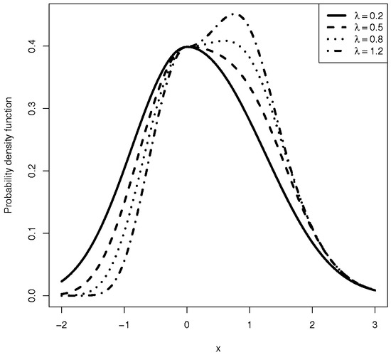
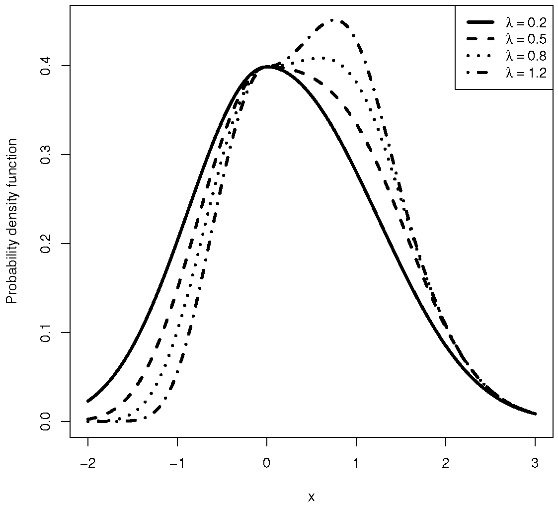
Figure 1. Plot of density function of BSN for different values of $\lambda$.

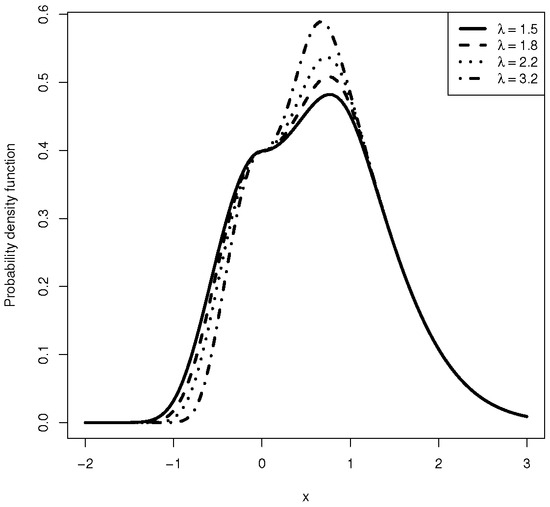
Figure 2. Plot of density function of BSN for different values of $\lambda$.

The BSN distribution, denoted by $Z\sim BSN\left(\lambda \right)$, is a distribution that is gaining attention as a valid competitor to the skew-normal model (SN) [1]. This is because both models control the degree of skewness using the same scalar parameter, $\lambda \in \mathbb{R}$. If $\lambda =0$, then the model is reduced to the symmetric normal model. However, as demonstrated in this study, a significant advantage of the BSN model over the SN model is that in the presence of the location parameter, the BSN information matrix is non-singular at $\lambda =0$. Consequently, under the null hypothesis of normality given by $H_0:\lambda =0$, the conventional regularity conditions leading to the ordinary asymptotic normal distribution of the MLE hold.

3.2. Some Basic Properties

Proposition 2 yields several important properties of the BSN distribution. First, if $Z\sim BSN\left(\lambda \right)$, then $-Z\sim BSN(-\lambda )$. This means that the distribution is symmetric with respect to the origin. Second, $Z^2\sim {\chi }_1^2$, which indicates that the distribution of the squared BSN variable follows a chi-squared distribution with one degree of freedom. Finally, $\left|Z\right|\sim HN(0,1)$, where $HN$ denotes the half-normal distribution. This property implies that the absolute value of a BSN variable follows an HN distribution with mean zero and variance one. These properties are useful for analyzing and interpreting data modeled with the BSN distribution.

3.2.1. Quantile Function

The quantile function of the BSN distribution is derived by inverting Equation (11), as follows:

$$Q_p=F_Z^{-1}(p;\lambda ),0<p<1.$$

(12)

This inverse does not have a closed expression and has to be calculated using some suitable numerical method. Note that $Q_{0.5}$, $Q_{0.25}$, and $Q_{0.75}$ stand for median, first quartile, and third quartile of the BSN distribution, correspondingly.

3.2.2. Moments, Skewness, and Kurtosis

The even moments of $Z\sim BSN\left(\lambda \right)$ are equal to the corresponding even moments of a standardized normal random variable. The odd moments can be computed from the result in Proposition 5, as follows:

$$\mathbb{E}\left(Z^{2k+1}\right)=2\mathbb{E}\left(Y^{2k+1}\mathsf{\Phi }\left(\lambda Y^2\right)\right)-{\displaystyle \frac{2^{1/2+k}}{\sqrt{\pi }}}\Gamma (k+1),k\in \{0,1,2,\dots \},$$

(13)

where $Y\sim HN(0,1)$. In particular, the first four moments are

$$\begin{array}{ccc}\hfill \mathbb{E}\left(Z\right)& =& {\displaystyle \frac{2}{\pi }}\rho \left(\lambda \right),\mathbb{E}\left(Z^2\right)=1,\hfill \\ \hfill \mathbb{E}\left(Z^3\right)& =& {\displaystyle \frac{2}{\pi {\lambda }^2}}\left[\lambda +{\displaystyle \frac{4{\lambda }^2-1}{2}}\rho \left(\lambda \right)\right],\mathbb{E}\left(Z^4\right)=3,\hfill \end{array}$$

where

$$\rho \left(\lambda \right)={\displaystyle \frac{\mathrm{sgn}\left(\lambda \right)}{\varphi \left(\frac{1}{2\left|\lambda \right|}\right)}}\left(1-\mathsf{\Phi }\left({\displaystyle \frac{1}{2\left|\lambda \right|}}\right)\right).$$

By using the moments above and the standard definitions, we can calculate the skewness and kurtosis of the BSN distribution directly.

3.2.3. Entropy

A measure of the uncertainty’s variation is the entropy of a random variable Z with a certain PDF. Greater data uncertainty is indicated by a high entropy value. The Rényi entropy [10], $R_{\alpha }\left(Z\right)$, for Z is defined as

$$R_{\alpha }\left(Z\right)={\displaystyle \frac{1}{1-\alpha }}log\left\{{\int }_{\mathbb{R}}{f}_Z^{\alpha }\left(z\right)dz\right\},$$

(14)

where $\alpha >0$ and $\alpha \ne 1$. Suppose Z has the BSN distribution; then, by substituting (9) in (14), we obtain

$$\begin{array}{ccc}\hfill {\int }_{\mathbb{R}}{f}_Z^{\alpha }\left(z\right)dz& =& {\int }_{-\infty }^0{2}^{\alpha }{\varphi }^{\alpha }\left(z\right){\mathsf{\Phi }}^{\alpha }(-\lambda z^2)dz+{\int }_0^{\infty }{2}^{\alpha }{\varphi }^{\alpha }\left(z\right){\mathsf{\Phi }}^{\alpha }\left(\lambda z^2\right)dz\hfill \\ & =& {\int }_0^{\infty }{2}^{\alpha }{\varphi }^{\alpha }(-z){\mathsf{\Phi }}^{\alpha }(-\lambda z^2)dz+{\int }_0^{\infty }{2}^{\alpha }{\varphi }^{\alpha }\left(z\right){\mathsf{\Phi }}^{\alpha }\left(\lambda z^2\right)dz\hfill \\ & =& 2^{\alpha }{\int }_0^{\infty }{\varphi }^{\alpha }\left(z\right)({\mathsf{\Phi }}^{\alpha }(-\lambda z^2)+{\mathsf{\Phi }}^{\alpha }\left(\lambda z^2\right))dz\hfill \end{array}$$

So, one obtains the Rényi entropy as follows:

$$R_{\alpha }\left(Z\right)={\displaystyle \frac{\alpha log\left(2\right)}{1-\alpha }}+{\displaystyle \frac{1}{1-\alpha }}log\left\{{\int }_0^{\infty }{\varphi }^{\alpha }\left(z\right)({\mathsf{\Phi }}^{\alpha }(-\lambda z^2)+{\mathsf{\Phi }}^{\alpha }\left(\lambda z^2\right))dz\right\}.$$

Shannon entropy [11] defined by $S_{\alpha }\left(Z\right)=\mathbb{E}\{-log\left(f_Z\left(z\right)\right)\}$ is the particular case of Equation (14) when $\alpha \to 1^{+}$. Both $R_{\alpha }\left(Z\right)$ and $S_{\alpha }\left(Z\right)$ do not have closed expressions and must be calculated using some suitable numerical method.

3.2.4. Order Statistics

Let $Z\sim BSN\left(\lambda \right)$ and $Z_1,Z_2,\dots ,Z_n$ be a random sample of independent and identically distributed variables with CDF $F_Z$ given in (11) and PDF $f_Z$ given in (9). Define the random variable $Z_{\left(1\right)}=min\{Z_1,Z_2,\dots ,Z_n\}$. It is known that the CDF of the sample minimum is given by

$$F_{Z_{\left(1\right)}}\left(y\right)=1-{(1-F_Z\left(y\right))}^n$$

and its PDF is

$$f_{Z_{\left(1\right)}}\left(y\right)=n{(1-F_Z\left(y\right))}^{n-1}{f}_Z\left(y\right).$$

On the other hand, define the random variable $Z_{\left(n\right)}=max\{Z_1,Z_2,\dots ,Z_n\}$. It is known that the CDF of the sample maximum is given by

$$F_{Z_{\left(n\right)}}\left(y\right)={\left(F_Z\left(y\right)\right)}^n$$

and its PDF is

$$f_{Z_{\left(n\right)}}\left(y\right)=n{\left(F_Z\left(y\right)\right)}^{n-1}{f}_Z\left(y\right).$$

In general, the PDF of the k-th-order statistic from a random sample of size n drawn from the distribution of Z is

$$f_{Z_{\left(k\right)}}\left(y\right)={\displaystyle \frac{n!}{(k-1)!(n-k)!}}{\left(F_Z\left(y\right)\right)}^{k-1}{(1-F_Z\left(y\right))}^{n-k}{f}_Z\left(y\right).$$

3.2.5. Maximum Likelihood Estimates for $\lambda$

The log-likelihood function for $\lambda$ can be defined for a random sample of size n from $Z\sim BSN\left(\lambda \right)$, as given below:

$$l(\lambda ,\mathbf{z})={\displaystyle \frac{n}{2}}log\left({\displaystyle \frac{2}{\pi }}\right)-{\displaystyle \frac{1}{2}}\sum _{i=1}^n{z}_i^2+\sum _{i=1}^{n}log\left(\mathsf{\Phi }\right(\lambda z_i|z_i|)),$$

(15)

where $\mathit{z}$ denotes the sample data. This log-likelihood function helps to estimate the parameter $\lambda$ of the BSN distribution. The likelihood equation induced from this function is given by

$${\displaystyle \frac{dl(\lambda ,\mathit{z})}{d\lambda }}=\sum _{i=1}^n{z}_i\left|z_i\right|{\displaystyle \frac{\varphi \left(\lambda z_i\right|z_i\left|\right)}{\mathsf{\Phi }\left(\lambda z_i\right|z_i\left|\right)}}=0.$$

(16)

The solution to this likelihood equation provides the MLE of $\lambda$ for the bimodal skew-normal distribution. The numerical values of $\widehat{\lambda }$ can be determined via any statistical software.

3.3. Simulation Study

In this section, we evaluate the effectiveness of the MLE method for estimating the parameter $\lambda$ in the BSN distribution. We generate random samples of various sizes: n = 50, 100, 150, and 200, keeping $\lambda$ fixed.

3.3.1. Generating Samples from BSN($\lambda$)

To generate random samples, follow these steps:

(i)

Set the parameter $\lambda$ and choose the sample size n.

(ii)

Generate a standard normal random variable $U\sim N(0,1)$.

(iii)

Compute $Y=\left|U\right|$.

(iv)

Generate a Bernoulli random variable S with success probability $p=\mathsf{\Phi }\left(\lambda Y^2\right)$.

(v)

Set $Z=Y$ if $S=1$, otherwise $Z=-Y$.

3.3.2. Analyzing $\lambda$ with MLE

After obtaining the samples, $\lambda$ is estimated using the MLE method. We assess the performance of this estimation by calculating the standard error (SE), bias, and mean square error (MSE) in $\mathsf{R}$ programming language [12]:

(i)

For a chosen $\lambda$, simulate a sample of size n as described.

(ii)

Estimate $\lambda$ using MLE.

(iii)

Repeat the above steps 1000 times.

(iv)

Compute the mean, SE, bias, and MSE of these 1000 estimates:

The mean, SE, bias, and MSE of $\widehat{\lambda }$ are given by

$$\begin{array}{ccc}\hfill \overline{\widehat{\lambda }}& =& {\displaystyle \frac{1}{1000}}\sum _{i=1}^{1000}{\widehat{\lambda }}_i,\hfill \\ \hfill {\mathrm{SE}}_{\overline{\widehat{\mathbf{\lambda }}}}& =& \sqrt{{\displaystyle \frac{1}{1000}}\sum _{i=1}^{1000}{({\widehat{\lambda }}_i-\overline{\widehat{\lambda }})}^2},\hfill \\ \hfill {\mathrm{bias}}_{\overline{\widehat{\lambda }}}& =& {\displaystyle \frac{1}{1000}}\sum _{i=1}^{1000}({\widehat{\lambda }}_i-\lambda )\hfill \end{array}$$

and

$${\mathrm{MSE}}_{\overline{\widehat{\lambda }}}={\displaystyle \frac{1}{1000}}\sum _{i=1}^{1000}{({\widehat{\lambda }}_i-\lambda )}^2,$$

respectively. Here, $\widehat{\lambda }$ represents the MLE of $\lambda$ for the ith iteration under a specific sample size n, $\overline{\widehat{\lambda }}$ corresponds to the mean of the parameter estimates obtained, for example, $\widehat{\lambda }{i}^{\prime }s$, and $\lambda$ denotes the actual value of the parameter.

Table 1 displays the mean estimates, SEs, biases, and MSEs of $\lambda$ for various sample sizes. The performance of the MLE was investigated for a wide range of initial values for $\lambda$, and in all cases, the MLE converged well. The results in Table 1 were obtained by setting the initial value of $\lambda$ to 1.00, irrespective of its actual value. Thus, any choice of initial value for $\lambda$ is expected to yield similar results, as shown in Table 1.

Table 1. Simulation  results.

Actual Value				Estimates
$\mathit{\lambda }$		$\mathit{n}$		$\overline{\widehat{\mathit{\lambda }}}$	${\mathbf{SE}}_{\overline{\widehat{\mathit{\lambda }}}}$	${\mathbf{bias}}_{\overline{\widehat{\mathit{\lambda }}}}$	${\mathbf{MSE}}_{\overline{\widehat{\mathbf{\lambda }}}}$
$-0.45$		50		$-0.5181$	0.2302	$-0.0681$	0.0576
		100		$-0.4867$	0.1460	$-0.0367$	0.0226
		150		$-0.4736$	0.1114	$-0.0236$	0.0130
		200		$-0.4658$	0.0951	$-0.0158$	0.0093
$-3.00$		50		$-3.7459$	2.3316	$-0.7459$	5.9874
		100		$-3.2822$	0.9619	$-0.2822$	1.0040
		150		$-3.1787$	0.7434	$-0.1787$	0.5841
		200		$-3.1211$	0.5792	$-0.1211$	0.3497
2.00		50		2.4008	1.2510	0.4008	1.7242
		100		2.1520	0.6375	0.1520	0.4291
		150		2.1191	0.4874	0.1191	0.2515
		200		2.0999	0.3808	0.0999	0.1548
1.30		50		1.4952	0.6503	0.1952	0.4606
		100		1.3923	0.3758	0.0923	0.1496
		150		1.3534	0.2686	0.0534	0.0749
		200		1.3426	0.2246	0.0426	0.0522
0.00		50		$6\times {10}^{-3}$	0.1333	$6\times {10}^{-3}$	0.0178
		100		$-1\times {10}^{-3}$	0.0832	$-1\times {10}^{-3}$	0.0069
		150		$-1\times {10}^{-3}$	0.0657	$-1\times {10}^{-3}$	0.0043
		200		$9\times {10}^{-4}$	0.0544	$9\times {10}^{-4}$	0.0030

Overall, Table 1 reveals that as n increases, the SEs, biases, and MSEs decrease, indicating that the MLE provides consistent estimates.

4. Practical Data Analysis

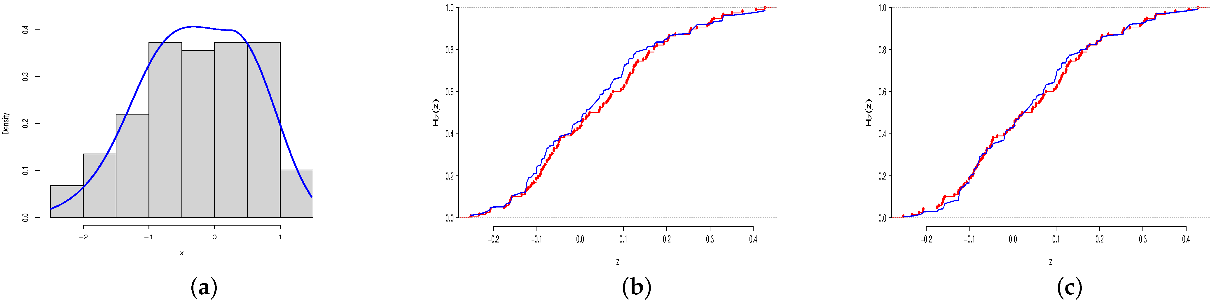
In this section, we illustrate the modeling capabilities of the BSN distribution by fitting it to 118 observations of the Homo sapiens PIG7 data in Çankaya [13] using the MLE method. To ensure computational stability, we scaled the data by $-0.171$ before fitting the distributions. The data are left-skewed with the Pearson’s moment coefficient of skewness of $-0.356576$ and appear to be bimodal, as seen in the empirical density plot in Figure 3a. Some of the descriptive statistics of the data include a minimum value of $-2.4971$, a maximum value of $1.4795$, a mean value of $-0.2512$, a variance value of $0.8162$, a median value of $-0.1930$, a first quartile value of $-0.8348$, and a third quartile value of $0.4678$. The resulting MLE of $\lambda$ is $-0.3676782$, with a corresponding SE of $0.1149803$. To assess the goodness-of-fit of the BSN distribution to the empirical data, we employed the Kolmogorov–Smirnov (K-S) test, with a test statistic defined as $D_n={\displaystyle \underset{1\le i\le k}{max}}(i/k-z_i,z_i-(i-1)/k)$, where $z_i$ is the ith data value. For large sample size n, the p-value of the K-S test is given by $P(\sqrt{n}{D}_n\le x)\approx {\displaystyle \frac{\sqrt{2\pi }}{\widehat{F}\left(z\right)}}{\sum }_{k=1}^{\infty }exp\left\{-{\displaystyle \frac{{(2k-1)}^2{\pi }^2}{8{\left[\widehat{F}\left(z\right)\right]}^2}}\right\}$, where $\widehat{F}\left(z\right)$ is the estimated CDF of the theoretical distribution, see Kolmogorov [14] and Smirnov [15]. The K-S test measures the disparity between the empirical and estimated cumulative distribution functions (CDFs), with a smaller difference indicating a better fit. In general, if the p-value of the K-S test is greater than $0.05$, we conclude that the model provides a good fit for the data. The fitted BSN distribution gives a K-S statistic of $0.10706$ with a p-value of 0.1337 (>0.05). Therefore, based on this evidence and visual inspection through the plot of the CDFs in Figure 3b, we conclude that the one-parameter BSN distribution provides a good fit for the data.

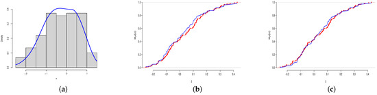
Figure 3. The plot of the empirical (rectangular bars) and estimated (blue line) PDF (a), estimated CDF of the uncentered BSN distribution (blue line) with the empirical CDF (red line) (b), and estimated CDF of the centered BSN distribution (blue line) with the empirical CDF (red line) (c).

We compare the fit of the BSN distribution with that of four other distributions, namely, the normal distribution, double Lindley distribution [16], Laplace distribution, and Student’s t-distribution. The PDFs of these distributions are as follows:

(i)

Normal distribution with PDF given by

$$f_X(x;\xi ,\eta )={\displaystyle \frac{1}{\eta }}\varphi \left({\displaystyle \frac{x-\xi }{\eta }}\right),x,\xi \in \mathbb{R},\eta >0,$$

where $\varphi \left(x\right)$ is the standard normal PDF.

(ii)

Double Lindley distribution with PDF given by

$$f_X(x;\lambda )={\displaystyle \frac{{\lambda }^2(1+|x\left|\right)}{2(\lambda +1)}}exp\{-\lambda |x\left|\right\},x\in \mathbb{R},\lambda >0.$$

(iii)

Laplace distribution with PDF given by

$$f_X(x;\xi ,\lambda )={\displaystyle \frac{1}{2\eta }}exp\left\{-{\displaystyle \frac{|x-\xi |}{\eta }}\right\},x,\xi \in \mathbb{R},\eta >0.$$

(iv)

Student’s t-distribution with PDF given by

$$f_X(x;\lambda )={\displaystyle \frac{{\left(1+\frac{x^2}{\lambda }\right)}^{-\frac{\lambda +1}{2}}}{\sqrt{\lambda }B\left(\frac{1}{2},\frac{\lambda }{2}\right)}},x\in \mathbb{R},\lambda >0,$$

where $B(a,b)$ is the beta function.

We used the K-S test to compare the goodness-of-fit of these distributions with that of the BSN distribution. The K-S test statistic measures the maximum distance between the empirical CDF of the data and the CDF of the fitted distribution, with a smaller test statistic indicating a better fit. The p-values of the K-S tests for each distribution were computed, and if the p-value was larger than $0.05$, we concluded that the distribution provided a good fit for the data.

To ensure a fair comparison between the fits of the normal distribution, Laplace distribution, and BSN distribution, it is important to center the BSN distribution about the mean ($\xi$), as both the normal and Laplace distributions are centered around the mean. To accomplish this, we introduce an additional parameter $\xi$ to the BSN distribution, resulting in a centered BSN distribution with PDF $2\varphi (x-\xi )\mathsf{\Phi }\left(\lambda \right(x-\xi \left)\right|x-\xi \left|\right)$ for $x,\xi ,\lambda \in \mathbb{R}$. To determine the best-fitting model for the data, we use the information criteria listed below along with the K-S test:

(i)

Akaike information criterion (AIC), given by AIC = $-2l\left(\widehat{\theta }\right)+2k$.

(ii)

Bayesian information criterion (BIC), given by BIC = $-2l\left(\widehat{\theta }\right)+klog\left(n\right)$.

(iii)

corrected AIC (AICc), given by AICc = AIC + ${\displaystyle \frac{2k(k+1)}{n-k-1}}$.

Here, $l\left(\widehat{\theta }\right)$ denotes the estimated log-likelihood value, n represents the number of data points, $\theta$ is the unknown parameter, and k indicates the number of parameters in the model. A smaller value of the information criterion indicates a better fit. Table 2 and Table 3 present the results of the fitted distributions. Based on these tables, we can observe that the centered BSN distribution outperformed all other considered distributions, with the smallest K-S statistic, largest p-value of K-S, and smallest values of AIC, BIC, and AICc. This is also evident from Figure 3c, where we can see that the CDF of the estimated centered BSN distribution closely mimics the empirical CDF.

Table 2. Fit results for different distributions.

		$\underset{\left[\mathbf{SE}\right]}{\mathbf{Parameter}\mathbf{Estimate}}$				K-S Test
Distribution		$\widehat{\mathit{\lambda }}$	$\widehat{\mathit{\xi }}$	$\widehat{\mathit{\eta }}$		$\mathit{D}$	$\mathit{p}$-Value
Normal		-	$\underset{\left[0.0828\right]}{-0.2512}$	$\underset{\left[0.0586\right]}{0.8996}$		0.0998	0.1903
BSN		$\underset{\left[0.3029\right]}{-0.7720}$	$\underset{\left[0.1130\right]}{0.2444}$	-		0.0837	0.3801
Double Lindley		$\underset{\left[0.1304\right]}{1.7862}$	-	-		0.1480	0.0114
Laplace		-	$\underset{\left[0.0331\right]}{-0.1293}$	$\underset{\left[0.0692\right]}{0.7521}$		0.1170	0.0791
Student’s t		$\underset{\left[104.4868\right]}{235,670.6}$	-	-		0.1187	0.0721

Table 3. Model fit discrimination.

				Information Criteria
Distribution		$-\mathit{l}\left(\widehat{\mathit{\lambda }}\right)$		AIC	BIC	AICc
Normal		154.9475		313.8951	319.4365	313.9994
BSN		151.2718		306.5435	312.0849	306.6479
Double Lindley		164.4999		330.9998	333.7704	331.0342
Laplace		166.1680		336.3361	341.8774	336.4404
Student’s t		159.9040		321.8079	324.5786	321.8424

In Table 4, descriptive statistics obtained from the empirical distribution and the estimated centered BSN distribution are compared. From the results, we can conclude that the fitted centered BSN distribution accurately captured the important features of the empirical distribution, as the first three moments and the standard deviation (std) of the estimated centered BSN distribution are similar to those of the empirical distribution. It is noteworthy that the direction of skewness is the same for both distributions. However, a slight difference in skewness values is observed, which may be due to rounding errors in the numerical integration of the k-th-order moments. The $\mathsf{R}$ code used to compute the descriptive statistics is provided in Appendix A.

Table 4. Some descriptive statistics for the empirical and centered BSN distributions.

		Moments
		${\mathit{\mu }}_{\mathit{1}}^{\prime }$	${\mathit{\mu }}_{\mathit{2}}^{\prime }$	${\mathit{\mu }}_{\mathit{3}}^{\prime }$		Std	Skewness
Empirical		−0.2512142	0.8723585	−0.8886568		0.903419	$-0.356576$
BSN		−0.2645494	0.8109423	−0.7589403		0.860788	−0.238893

5. Concluding Remarks

In this study, we introduced a new family of continuous distributions known as bimodal skew-symmetric distributions. The BSN distribution, which is essential to this family, is distinguished by the single parameter that causes its asymmetry. The statistical properties of this distribution have been thoroughly discussed, emphasizing its flexibility and applicability.

Utilizing the MLE method, we estimated this sole asymmetry parameter, demonstrating the practicality and effectiveness of the BSN model when applied to real-world data. The analysis highlights the BSN distribution’s capability to adeptly model data features, such as skewness and bimodality, which are often encountered in practical datasets but are challenging to address with more traditional models.

To enhance the utility of the BSN distribution and facilitate its comparison with more conventional distributions like the normal and Laplace distributions, both of which are two-parameter models centered about the mean, we plan to extend the BSN distribution by centering it about the mean in future applications. This adjustment will allow the BSN distribution to be directly comparable to these models, providing a fair basis for performance evaluation.

The results from this study are promising, showing that the two-parameter BSN distribution not only meets but exceeds the performance of the four considered competing distributions for the dataset in question. This superior performance underscores the potential of the BSN distribution as a robust and versatile tool in statistical modeling, particularly suitable for complex real-world data that exhibit asymmetry and bimodality.

This study contributes to an application of bimodal skew-symmetric distributions to the analysis of cancer cell protein data, addressing the inherent bimodality and asymmetry of such data. The proposed model enhances the flexibility and accuracy of statistical representations, leading to improved parameter estimation and robust analysis even in the presence of noise. By incorporating regularization techniques to prevent singularity issues and leveraging the model’s adaptability to capture complex biological variability, this research provides an effective tool for identifying subpopulations and characterizing protein profiles in cancer cells. These contributions not only advance the field of statistical modeling in bioinformatics but also have practical implications for biomarker discovery and proteomics analysis, paving the way for more precise and meaningful insights into cancer biology.

The implications of these findings are significant, suggesting that the BSN distribution can serve as an alternative to traditional models, offering enhanced flexibility and better fit for specific types of data. Future studies will focus on further developing this model, improving its statistical inference procedures, and extending its application to a broader range of datasets.

References

- Azzalini, A. A class of distributions which includes the normal ones. Scand. J. Stat. 1985, 12, 171–178. [Google Scholar]
- Azzalini, A. Further results on a class of distributions which includes the normal ones. Statistica 1986, 46, 199–208. [Google Scholar]
- Gupta, A.K.; Chang, F.C.; Huang, W.J. Some skew–symmetric models. Random Oper. Stoch. Equ. 2002, 10, 113–140. [Google Scholar] [CrossRef]
- Ma, Y.; Genton, M.G. Flexible class of the skew-symmetric distributions. Scand. J. Stat. 2004, 31, 459–468. [Google Scholar] [CrossRef]
- Arellano-Valle, R.B.; Gómez, H.W.; Quintana, F.A. A new class of skew-normal distributions. Commun. Stat. Theory Methods 2004, 33, 1465–1480. [Google Scholar] [CrossRef]
- Pewsey, A. Some observations on a simple means of generating skew distributions. In Advances in Distribution Theory, Order Statistics, and Inference Part of the Series Statistics for Industry and Technology; Springer: New York, NY, USA, 2006; pp. 75–84. [Google Scholar]
- Bakouch, H.S.; Salinas, H.S.; Mamode Khan, N.; Chesneau, C. A new family of skewed distributions with application to some daily closing prices. Comput. Math. Methods 2021, 3, e1154. [Google Scholar] [CrossRef]
- Salinas, H.; Bakouch, H.; Qarmalah, N.; Martínez-Flórez, G. A flexible class of two-piece normal distribution with a regression illustration to biaxial fatigue data. Mathematics 2023, 11, 1271. [Google Scholar] [CrossRef]
- Khorsheed, E.; Salinas, H.S.; Bakouch, H.S. A new family of skew-normal lifetime distributions for industrial applications. In Proceedings of the 2020 International Conference on Data Analytics for Business and Industry: Way Towards a Sustainable Economy (ICDABI), Sakheer, Bahrain, 26–27 October 2020; pp. 1–4. [Google Scholar]
- Rényi, A. On measures of information and entropy. In Proceedings of the 4th Berkeley Symposium on Mathematical Statistics and Probability, Los Angeles, CA, USA, 20–30 June 1960; Neymann, J., Ed.; University of California Press: Berkeley, CA, USA, 1961; pp. 547–561. [Google Scholar]
- Shannon, C.E. A mathematical theory of communication. Bell. Syst. Tech. J. 1948, 27, 379–423. [Google Scholar] [CrossRef]
- R Core Team. R: A Language and Environment for Statistical Computing; R Foundation for Statistical Computing: Vienna, Austria, 2024; Available online: https://www.R-project.org/ (accessed on 10 January 2024).
- Çankaya, M.N. Asymmetric bimodal exponential power distribution on the real line. Entropy 2018, 20, 23. [Google Scholar] [CrossRef] [PubMed]
- An, K. Sulla determinazione empirica di una legge didistribuzione. Giorn. Dell’inst. Ital. Degli Att. 1933, 4, 89–91. [Google Scholar]
- Smirnov, N. Table for estimating the goodness of fit of empirical distributions. Ann. Math. Stat. 1948, 19, 279–281. [Google Scholar] [CrossRef]
- Nitha, K.; Krishnarani, S. A new family of heavy tailed symmetric distribution for modeling financial data. J. Stat. Appl. Probab. 2017, 6, 577–586. [Google Scholar]
Disclaimer/Publisher’s Note: The statements, opinions and data contained in all publications are solely those of the individual author(s) and contributor(s) and not of MDPI and/or the editor(s). MDPI and/or the editor(s) disclaim responsibility for any injury to people or property resulting from any ideas, methods, instructions or products referred to in the content. |
© 2024 by the authors. Licensee MDPI, Basel, Switzerland. This article is an open access article distributed under the terms and conditions of the Creative Commons Attribution (CC BY) license (https://creativecommons.org/licenses/by/4.0/).