Frequency-Enhanced Transformer with Symmetry-Based Lightweight Multi-Representation for Multivariate Time Series Forecasting

Abstract

Transformer-based methods have recently demonstrated their potential in time series forecasting problems. However, the mainstream approach, primarily utilizing attention to model inter-step correlation in the time domain, is constrained by two significant issues that lead to ineffective and inefficient multivariate forecasting. The first is that key representations in the time domain are scattered and sparse, resulting in parameter bloat and increased difficulty in capturing time dependencies. The second is that treating time step points as uniformly embedded tokens leads to the erasure of inter-variate correlations. To address these challenges, we propose a frequency-wise and variables-oriented transformer-based method. This method leverages the intrinsic conjugate symmetry in the frequency domain, enabling compact frequency domain representations that naturally mix information across time points while reducing spatio-temporal costs. Multivariate inter-correlations can also be captured from similar frequency domain components, which enhances the variables-oriented attention mechanism modeling capability. Further, we employ both polar and complex domain perspectives to enrich the frequency domain representations and decode complicated temporal patterns. We propose frequency-enhanced independent representation multi-head attention (FIR-Attention) to leverage these advantages for improved multivariate interaction. Techniques such as cutting-off frequency and equivalent mapping are used to ensure the model’s lightweight nature. Extensive experiments on eight mainstream datasets show that our approach achieves first-rate satisfactory results and, importantly, requires only one percent of the spatio-temporal cost of mainstream methods.

1. Introduction

Multivariate time series forecasting has a wide range of applications in a multitude of real-world fields and plays a crucial role in many aspects of life [1,2,3,4]. In mainstream application areas such as energy [5], weather [6,7], electricity [8,9], traffic [10,11] and finance [12,13], it is not only necessary to consider the historical data and changing trend of a single variable but also, more importantly, to gain insight into the interactions and synergistic effects of the variables to bring about better prediction performance. For example, in meteorological forecasting, the combination of temperature and humidity can influence precipitation, changes in wind speed and air pressure are the key to predicting storms, and various variables exert an effect on the temperature indicator, which is of the greatest concern to residents.

As the transformer is capable of efficiently extracting semantic correlations between pairs of elements in a long sequence based on the self-attention mechanism, it has been widely used in multivariate time series forecasting in recent years [14,15,16]. However, existing points-oriented transformer methods that use time steps or frequency components as tokens and then use the attention mechanism to model the correlation for different moments have some drawbacks (represented by the Informer [17] and FEDformer [18]). First, unlike natural language, where each word token possesses abundant and independent semantic information, in the time series domain, individual time step tokens without contextual connections tend to lack semanticity. Second, for time series analysis, capturing temporal dependencies of a sequential nature across time steps is an essential aspect, and attention (with its permutation-invariant and anti-ordering nature) contradicts this necessity to a certain extent. Third, for multivariate time series forecasting, each variable represents a different subject of observation or physical quantity, which has completely different meanings in reality and units of measurement [19]. An improved scheme, proposed by iTransformer [20], uses time series variables as tokens, models multivariate correlation using the attention mechanism, and obtains temporal dependencies via subsequent feedforward neural networks, encoding historical observations layer by layer. Although this approach addresses some of the shortcomings of the single time step token scheme, there are still some limitations and bottlenecks involved in the original time domain compared with the frequency domain perspective we adopt herein.

Specifically, time series data typically display inefficiencies within the time domain representation, characterized by redundancy and less efficient information encoding compared to the frequency domain. In the frequency domain, signals enable lossless reconstruction, which is more streamlined due to the inherent symmetry and compactness of frequency-based methods. This challenge is intensified by the high-dimensional mapping from variable sequence lengths to hidden dimensions, typically ranging from 96 to 512. Frequency domain representations offer a more compact and efficient scheme, leveraging symmetry-based frequency shifts to reduce dimensional overhead and enhance data representation succinctness. Moreover, valid information in the time domain tends to be scattered and sparse, with significant events like trend transitions or critical fluctuations sparsely represented across time steps. Each time step, treated independently and uniformly, lacks interconnectedness and cohesive structure. In contrast, the frequency domain perspective leverages the inherent conjugate symmetry in Fourier transforms, blending information from all sequence time steps and viewing the sequence holistically. This exploitation of symmetry not only ensures a more compact representation but also enhances data processing efficiency by reducing the number of computations required for transformations. This is especially advantageous for capturing the inherent patterns of the series, making the frequency domain ideal for expressing dynamics that are obscured in the time domain. Finally, for multivariate time series data, the dependencies among variables are often manifested through similar periodic patterns and causal fluctuations. In the frequency domain, these dependencies are more intuitively captured as variables often share similar frequency components. This provides a clearer and more insightful perspective than is typically possible with time domain analysis, making it easier to detect and interpret underlying relationships.

Summarizing our research motivation and problem definition, we identified two main types of challenges to current approaches. The existing state of the research area is described in further detail in Section 2, Related Work. Here, they are briefly distilled into the following two points, which highlight the need to reform the methodology:

• Points-Oriented Limitations: Embedding multiple variables at the same time step into a single token obscures distinct physical properties and undermines the ability to capture critical inter-variable correlations, thus complicating the effective modeling of variable dependencies.
• Time-Wise Limitations: time domain representations are characterized by inefficiency and redundancy, with critical information often dispersed and sparse across time steps. This results in a lack of cohesive structure, making it difficult to capture and utilize significant temporal patterns effectively.

Therefore, we innovatively propose a variables-oriented and frequency-wise attention modeling method and propose some elements of design to increase the advantages of this scheme. Within this framework, in addition to compact frequency domain representations, we employ frequency cutting and equivalent mapping mechanisms to allow the computational and memory consumption of attention with quadratic complexity to be significantly reduced. Furthermore, in order to enhance the representation capability in the frequency domain and the modeling of complex temporal patterns, we propose frequency-enhanced independent representation multi-head attention (FIR-Attention). As shown in Figure 1, we incorporate the prior frequency-wise knowledge and experience into the design of the attention mechanism and use the magnitude, phase, and real/imaginary parts of two sets of complete frequency domain representations (the polar representation and complex representation) as the predefined objects to be processed by the four sub-heads. Independent sub-heads are assigned responsibility for one of the frequency domain representations, relying on attention computation to capture relevant dependencies after interference-free query, key and value mapping. As a result, we adopt multiple representations to enhance the frequency-wise performance and use attention for multivariate interactions under lightweight conditions to achieve comprehensive frequency domain modeling outcomes and high-precision time domain forecasting. Our contribution can be summarised as follows:

Figure 1. Frequency domain multiple representations of time series for frequency-wise attention. The polar representation of magnitude and phase and the complex representation of real and imaginary parts. Due to the inherent conjugate symmetry in the frequency domain, only half of the spectrum is displayed, showcasing the efficiency of symmetry-based reductions. The right part illustrates the corresponding attention map of the frequency representation, highlighting how different frequency components are weighted for analysis.

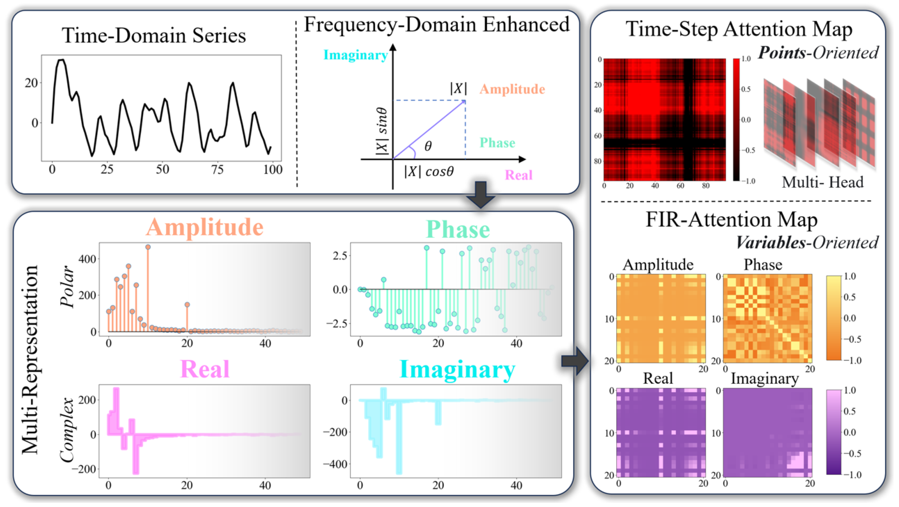
• We propose a transformer-based frequency-enhanced multivariate time series forecasting method. It takes a compact frequency-wise perspective and uses attention to capture the correlation dependence of frequency domain representations of multivariate interactions.
• We adopt a cutting-off frequency and an equivalent mapping design to ensure the efficiency and lightweightness of the model. Further, we propose FIR-Attention to construct rich frequency representations and reliable attention computation from polar and complex-valued domains.
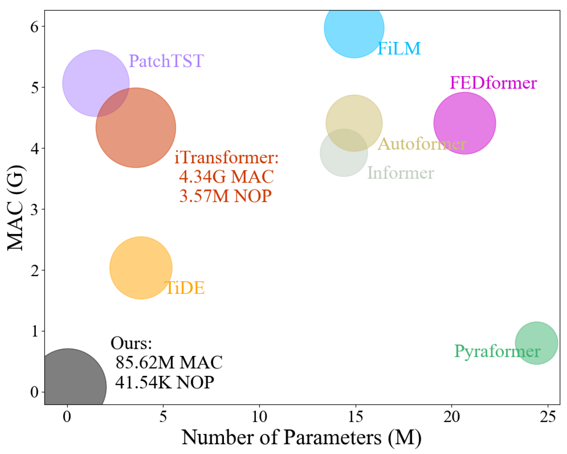
• Extensive experiments demonstrate that our method achieves similar or even better prediction performance than mainstream transformer-based models with only one percent of space–time consumption. The novel idea of FIR-Attention and two spatial compression schemes are also proven effective.

The rest of this paper is organized as follows. First, we introduce the existing related work, detail our motivation, and propose an improved approach based on variables-oriented and frequency-wise attention in Section 2. Then, we describe the details of the proposed model in Section 3 and show the extensive experimental results in Section 4. Finally, we draw a brief conclusion in Section 5.

2. Related Work

In this section, we explore the landscape of time series forecasting methods within the realm of deep learning, focusing particularly on the evolution from traditional models to the latest advancements in transformer-based techniques. We begin with a review of conventional deep learning methods, such as RNNs and CNNs, discussing their strengths, limitations, and how they compare to contemporary transformer approaches. We then delve deeper into transformer-based methods, dissecting core concepts such as points-oriented versus variable-oriented and time-wise versus frequency-wise approaches, which are crucial for understanding the existing gaps that our proposed method aims to address. Finally, we discuss frequency-aware analysis models, highlighting past efforts and setting the stage for our contributions in enhancing multi-representation in the frequency domain. This structured overview not only contextualizes our work within the broader field but also delineates the scholarly motivations and problem definitions that our research addresses.

2.1. Deep Learning Forecasting Methods

Statistical methods such as autoregressive moving average(ARMA), seasonal autoregressive moving average (SARIMA) and exponential smoothing rely on the statistical properties of the data [21]. These methods typically assume that the data follow specific statistical distributions and use the parameters of these distributions to make predictions. In the real world, however, many time series data exhibit complex non-linear and non-stationary characteristics, and classical models perform poorly in these cases and are more sensitive to outliers, which may lead to degraded forecasting performance [22,23,24]. Forms of deep learning architecture, proven to be effective, have been widely used in time series prediction tasks and have achieved breakthrough performance [25]. Recurrent neural networks (RNNs) are particularly suitable for processing sequential data, can effectively capture time dependencies, and can enhance the expressive of the model by modifying the network structure, e.g., LSTMs [26,27,28] or GRUs [29], which use a gate mechanism to avoid the gradient vanishing problem [30]. However, in practice. training is still complex and computationally intensive, and for very long sequences, even LSTM and GRU may have difficulty in capturing early information [31]. Convolutional neural networks (CNNs) can automatically extract locally important features in time series through multi-layer convolution and are suitable for parallel computing, which can significantly improve training efficiency [32,33]. However, CNNs mainly capture local features and may not be sensitive enough to the time series features that need to be understood globally, and in the face of long sequences that need to be stacked with multiple layers of convolution, they also face the problem of long-range dependence capture [34].

The transformer model is able to capture the dependency between any two points in a sequence through the self-attention mechanism, which is particularly suitable for processing long sequences of data, and the model can be easily extended to process time series data or modified to suit different task requirements. Unlike the step-by-step computation of RNN, the transformer allows data to be processed simultaneously in various parts of the model, significantly increasing the training speed [14,35]. Despite the high degree of parallelization, the quadratic complexity of attention also consumes relatively large computational and storage resources, which often becomes a bottleneck, especially when dealing with large-scale datasets [36]. Modifying the original transformer design to make it more suitable for time series prediction has become a hot research topic in recent years [37].

2.2. Transformer-Based Methods

As the transformer model continues to break through in the fields of natural language processing and computer vision, the powerful sequence modeling and information interaction capabilities of this architecture have been fully demonstrated [38,39]. Its potential in the field of time series forecasting has also been well explored by the well-designed variants of the transformer-based model [40,41,42]. Through a systematic review of transformer-based forecasting schemes, we hypothesize that existing mainstream transformer-based methods can be broadly classified into four categories based on attention oriented to a point or variable, dealing with either the time domain or frequency domain, as shown in Figure 2.

Figure 2. The four attention approaches that existing transformer-based works are based on, being either points- or variables-oriented and dealing with the time or frequency domain. (a) refers to a time-wise and points-oriented method, represented by the informer [17]. (b) refers to a frequency-wise and points-oriented method, represented by the FEDformer [18]. (c) refers to a time-wise and variables-oriented method, represented by the iTransformer [20]. (d) refers to a frequency-wise and variables-oriented method, representing our approach. The grey parts show the frequency of screening out in order to further compact and thus reduce consumption and increase efficiency.

First, in the classical approach, as in Figure 2a, attention is points-oriented to deal with the time domain. This type of approach is inherited from vanilla transformer’s sequential modeling architecture, where attention is oriented to correlation interactions and dependency capturing for each temporal step under the time domain. A large number of models adopt points-wise or series-wise ideas while trying to reduce $O\left(L^2\right)$ time and memory complexity. LogTrans [43] proposed the LogSparse attention mechanism, which selects time steps to follow exponentially growing intervals in order to reduce the time and memory consumption of quadratic complexity. Pyraformer [44] employs a pyramidal attention mechanism that is capable of capturing hierarchically multi-scale temporal dependencies with an $O\left(L\right)$ time and memory complexity. Informer [17] adapts the transformer using distillation mechanisms and the ProbSparse attention based on the KL-divergence approach, thereby achieving a similar $O\left(LlogL\right)$ complexity. Autoformer [45] developed a series-wise auto-correlation mechanism that models the sub-sequence correlations to replace the original attention layer to achieve $O\left(LlogL\right)$ complexity. Performer [46] proposes the MSSC mechanism and predictive paradigm as a replacement for the typical point attention mechanism, with the aim of improving efficiency and extracting more information.

While the transformer is arguably the most efficient way of extracting semantic associations between elements in long sequences, it is obviously suitable for making predictions by capturing associations between individual points in time. However, in sequence modeling, extracting temporal relationships in an ordered set of sequential points is a much more important matter. Specifically, unlike the field of natural language, where individual points are semantically rich, in the field of time series, individual points out of context do not have valid information. The amount of information contained in a temporal token of a point in time is more limited, meaning that working from temporal tokens may not be conducive to modeling global temporal correlations.

Secondly, in exploratory approaches, as in Figure 2b, attention is points-oriented to deal with the frequency domain. This type of approach is similar to time step modeling, with the difference that attention is oriented to the frequency domain to deal with the dependency interactions between each frequency component. The most representative is FEDformer [18], which takes the frequency domain information as the main target of attention capture, and the object of the correlation interaction is the amplitude of the randomly selected frequency pattern. The computational complexity can be reduced to $O\left(LlogL\right)$ due to the use of fast Fourier transform (FFT), and the model uses only a random subset of the Fourier basis, the scale of which is bounded by a scalar; its computational complexity can be further reduced to $O\left(L\right)$.

The frequency domain perspective can be seen as mixing information from various data points in the time domain. However, such approaches suffer from the same limitations as the previous category in terms of token design and interaction between objects of attention. That is, the attention mechanism is naturally permutation-invariant and anti-ordering, which conflicts with the requirements of time series modeling [19]. In addition, in terms of token encoding, for data points of different variables at the same time step or frequency, they have different physical meanings and different measurement scales. This forces them to be embedded as uniform temporoal tokens without distinguishing different variable channels which would result in the elimination of correlation between multiple variables. Furthermore, embedding multiple variables from each point into the same token may lead to meaningless learned attention maps, failure to obtain efficient variable-based representations, which in turn leads to unsuitability for multivariate temporal prediction tasks [20].

Third, in recently popular approaches, as in Figure 2c, attention is variables-oriented to deal with the time domain. iTransformer [20] presents an inverted view of the first category of transformer methods. It maps each variable rather than time step into a high-dimensional feature representation encoded into independent tokens, with the variable as the subject of description. More importantly, the correlation between different variables is modeled using the attention mechanism to effectively capture inter-variable dependencies. The feedforward network then encodes the features of historical observations in the time dimension and maps the learned features into future predictions.

Although this approach provides an effective attention idea for variable interactions, it is also limited by the high spatial and temporal complexity of the original attention model, especially in the face of ultra-long sequences that may lead to large consumption of computational resources. Critical serial variations are only in a few sequential time steps, and the original time domain representations are often relatively redundant, making computational efficiency a bottleneck. Compact frequency domain representations not only alleviate this problem; the frequency-wise method naturally mixes information from all points in time as components, especially for transitions and fluctuations that are important for time series modeling.

Finally, in our approach, as in Figure 2d, attention is variables-oriented to deal with the frequency domain. Information fusion is performed by capturing global frequency features through a compact frequency domain representation, thus simplifying the redundancy problem in the time domain, an element of efficiency that is particularly important when dealing with large or long time series data. More significantly, our approach treats variables as attention correlation interaction objects, effectively capturing inter-variable dependencies from the frequency domain perspective. The special independent sub-head attention design also allows multiple frequency domain features to provide different perspectives and information from the time domain, which helps to improve the performance and robustness of the model. The design of frequency domain filtering and equivalent mapping also makes the compact frequency domain attention computation more efficient.

2.3. Frequency-Aware Analysis Model

The frequency domain analysis is commonly employed to enhance the model features. This analytical technique is a pivotal instrument in methodologies such as frequency component selection, spectral data computation, information point mixing, and noise reduction. Additionally, it is frequently utilized to discern patterns inherent in the data.

FNet [47] enables token information interaction by replacing the attention layer with a standard parameter-free Fourier transform. The principle followed is that each element generated by the Fourier transform is a fusion of all the token information in the original sequence, thus enabling token mixing. It does not require convolutional layers, recurrence layers and attentional computation, thus greatly improving the operating efficiency on the GPU. Autoformer argues that similar phases of different periods usually exhibit similar sub-processes between them, and proposes autocorrelation mechanisms to achieve efficient series-level connectivity and thus extend the information’s utility. The autocorrelation coefficient calculation based on the Wiener–Khinchin theory is obtained by the fast Fourier transform (FFT) in the frequency domain [45]. TimesNet [48] models this by identifying a specified number of dominant frequencies to infer possible periodic patterns then segments and stacks the sequence accordingly. Specifically, a fast Fourier transform (FFT) is used to find frequencies with more significant amplitudes, and based on their periodic patterns, the original one-dimensional time series is reshaped into a two-dimensional image of the same period, which is then converted into a convolutional algorithm. FEDformer [18], arguing that most time series tend to have sparse representations in well-known bases (e.g., Fourier transforms), randomly selects a subset of frequency components including both low-frequency components and high-frequency components. Linear computational complexity and memory overhead is achieved by selecting a fixed number of Fourier components and subsequently interacting with each selected Fourier component via frequency attention. In addition, wavelet bases, which are more dominant in capturing local structure in a time series compared to Fourier bases, can be used as an alternative. FITS [49] employs a linear neural network capable of handling complex values to obtain a more comprehensive representation of time series by modeling the transformation information in the frequency domain. The linear structure for the frequency domain brings high efficiency with low memory consumption, making it suitable for deployment in edge devices. FiLM [50] proposes a frequency-improved Legendre memory model by combining Fourier analysis and a low-rank matrix approximation to introduce a dimensionality reduction layer to reduce the influence of noise signals on the Legendre projection and to speed up the computation. After pre-processing the sequence information using the Legendre projection, the temporal information is mixed and modelled by multiple scales in the frequency domain perspective.

Existing time series forecasting studies have extensively used the frequency domain as a method of analysis and modeling, but the exploitation of spectral data richness remains unexplored. Specifically, models are often limited to the amplitude spectrum when capturing information in the frequency domain, and features in other frequency domains are not fully explored. Our method, meanwhile, divides the frequency domain into two groups: the complex representation and the polar representation. The correlation between variables is calculated using the independent sub-head attention from both real and imaginary parts as well as amplitude and phase perspectives. At the same time, the results of variable interactions in the real and imaginary parts are interpolated and filled with complex-valued mapping layers to complete the time relationship capture, which is efficient and accurate. The enriched frequency domain characterization allows the model to capture and analyze all the characteristics of the signal more comprehensively and precisely, thus providing better performance and higher adaptability in a variety of applications.

3. Methodology

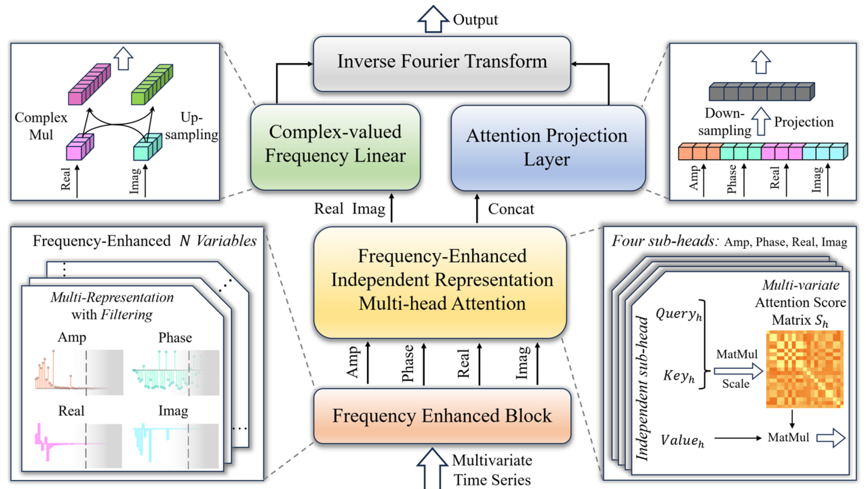
3.1. Overview of the Algorithm

The overall structure of our method is demonstrated in Figure 3. The abundant frequency domain representations of the time series are first obtained by the frequency-enhanced block. Subsequently, the magnitude, phase, real and imaginary parts are used as an independent sub-head of frequency-enhanced independent representation multi-head attention (FIR-Attention) to capture the multivariate interactions under each frequency domain feature. Among them, the independent query, key, and value mappings ensure that the frequency domain features do not interfere with each other in variable correlation capture. FIR-Attention outputs the interaction results of each independent sub-head, where the real and imaginary parts are up-sampled and interpolated by complex-valued frequency linear (CFLinear). In addition, the interaction results of each independent sub-head are concatenated and then down-sampled and projected to complete the union across frequency domain features to learn the optimal frequency domain combinatorial mapping. Finally, the weighted sum of the two together forms the prediction result. In this subsection, we describe the pipeline of our method. In the following two subsections, we describe in detail FIR-Attention, which handles multivariate dependencies, and CFLinear, which handles complex-valued mappings.

Figure 3. The overall structure of our method.

In the frequency-enhanced block, we first apply the discrete Fourier transform (DFT) to the time domain sequence $\mathbf{x}\in {\mathbb{R}}^{B\times N\times T}$ of normalised to zero-means, where B denotes the batch size, N represents the number of variables, and T is the sequence length. This transformation yields the frequency domain representation $\mathbf{X}\in {\mathbb{C}}^{B\times N\times (T/2+1)}$, where each element $\mathbf{X}[b,n,k]$ is a complex number representing the Fourier coefficient at frequency index k for the n-th variable in the b-th batch:

$$\mathbf{X}[b,n,k]=\sum _{t=0}^{T-1}\mathbf{x}[b,n,t]·e^{-j\frac{2\pi kt}{T}},k=0,1,\dots ,T/2,\forall b,n$$

(1)

Here, j is the imaginary unit. Then, we apply a low-pass filtering operation to the frequency domain representation $\mathbf{X}$ by retaining only the lowest $C=\lceil \eta \ast T\rceil$ frequency components and discarding the higher frequencies, where $\eta$ is a hyper-parameter ranging from 0 to 0.5. To achieve this, we construct a mask matrix $\mathbf{M}\in {\mathbb{R}}^{B\times N\times (T/2+1)}$, such that

$$\mathbf{M}[b,n,k]=\left\{\begin{array}{cc}\hfill 1,\hfill & \hfill \mathrm{if}k\le C\hfill \\ \hfill 0,\hfill & \hfill \mathrm{otherwise}\hfill \end{array}\right.$$

(2)

The low-pass-filtered frequency domain representation ${\mathbf{X}}_{low}$ is obtained by element-wise multiplication of $\mathbf{X}$ and $\mathbf{M}$:

$${\mathbf{X}}_{low}=\mathbf{X}\odot \mathbf{M}$$

(3)

This low-pass filtering operation is commonly employed to remove high-frequency noise and retain the dominant low-frequency components of the signal, which often carry the most relevant information for various time series analysis tasks. We crop it to the effective data size, such that ${\mathbf{X}}_{low}\in {\mathbb{C}}^{B\times N\times C}$. The effects from the low-pass filter are discussed in the experimental Section 4.3.4. Subsequently, we represent the low-pass filtered frequency domain data ${\mathbf{X}}_{low}$ in complex form as:

$${\mathbf{X}}_{low}[b,n,c]=\mathbf{R}[b,n,c]+j\mathbf{I}[b,n,c]$$

(4)

In the frequency domain representation of the low-pass filtered frequency components, $\mathbf{R}[b,n,c]$ and $\mathbf{I}[b,n,c]$ denote the real and imaginary parts, respectively, of the Fourier coefficient at frequency index c for the n-th variable in the b-th batch. We can further compute the amplitude $\mathbf{A}[b,n,c]$ and phase $\mathbf{P}[b,n,c]$ of this frequency component as follows:

$$\begin{array}{cc}\hfill \mathbf{A}[b,n,c]& =\left|{\mathbf{X}}_{low}[b,n,c]\right|=\sqrt{\mathbf{R}{[b,n,c]}^2+\mathbf{I}{[b,n,c]}^2}\hfill \\ \hfill \mathbf{P}[b,n,c]& =\angle {\mathbf{X}}_{low}[b,n,c]={tan}^{-1}\left(\frac{\mathbf{I}[b,n,c]}{\mathbf{R}[b,n,k]}\right)\hfill \end{array}$$

(5)

In our implementation, we utilize these four frequency domain features (amplitude $\mathbf{A}$, phase $\mathbf{P}$, real part $\mathbf{R}$, and imaginary part $\mathbf{I}$) as the independent input of the attention heads’ input to FIR-Attention to capture variable patterns in different frequency features:

$${\mathbf{O}}_{\mathrm{Attention}},{\mathbf{O}}_{\mathrm{Real}},{\mathbf{O}}_{\mathrm{Imag}}=FIR-Attention(\mathbf{A},\mathbf{P},\mathbf{R},\mathbf{I}),$$

(6)

where the output ${\mathbf{O}}_{\mathrm{Attention}}$ concatenates the inter-variable interaction results for all frequency-wise features. ${\mathbf{O}}_{\mathrm{Real}}$ and ${\mathbf{O}}_{\mathrm{Imag}}$ are two independent sub-head outputs of FIR-Attention, preserving pure real and imaginary parts’ detailed information while capturing variable dependencies.

Next, the attention projection layer performs down-sampling mapping and projection of ${\mathbf{O}}_{\mathrm{Attention}}$ through a multi-layer perceptron (MLP) [51] to ensure dimensional consistency. Meanwhile, complex-valued frequency linear (CFLinear) layer performs differential mapping and up-sampling operations on ${\mathbf{O}}_{\mathrm{Real}}$ and ${\mathbf{O}}_{\mathrm{Imag}}$ to produce an up-sampled complex-valued representation. This layer takes advantage of the nature of complex signals to simulate the effect of frequency shifting, thus achieving up-sampling prediction in the frequency domain:

$$\begin{array}{cc}\hfill {\mathbf{O}}_{\mathrm{Attention}}^{\mathrm{down}}& =MLP\left({\mathbf{O}}_{\mathrm{Attention}}\right)\hfill \\ \hfill {\mathbf{O}}_{\mathrm{Complex}}^{\mathrm{up}}& =CFLinear({\mathbf{O}}_{\mathrm{Real}},{\mathbf{O}}_{\mathrm{Imag}})\hfill \end{array}$$

(7)

Lastly, we perform the inverse Fourier transform ${\mathcal{F}}^{-1}$ on ${\mathbf{O}}_{\mathrm{Complex}}^{\mathrm{up}}$ and ${\mathbf{O}}_{\mathrm{Attention}}^{\mathrm{down}}$ and weight the results to obtain the final prediction result ${\mathbf{O}}_{\mathrm{Pred}}$.

$${\mathbf{O}}_{\mathrm{Pred}}=\alpha {\mathcal{F}}^{-1}\left({\mathbf{O}}_{\mathrm{Complex}}^{\mathrm{up}}\right)+\beta {\mathcal{F}}^{-1}\left({\mathbf{O}}_{\mathrm{Attention}}^{\mathrm{down}}\right),$$

(8)

where $\alpha$ and $\beta$ are weighting coefficients used to normalise the frequency domain amplitudes and energy levels during up-sampling and down-sampling, and they are typically ratios of the prediction length to the processing dimension.

3.2. Frequency-Enhanced Independent Representation Multi-Head Attention

FIR-Attention takes four frequency domain features as input, which collectively describe the complete information of each frequency component. These features reflect different semantics and can provide the model with richer frequency domain knowledge. The amplitude $\mathbf{A}$ represents the strength or energy of the frequency component, reflecting its importance in the sequence. The phase $\mathbf{P}$ denotes the phase angle of the frequency component, reflecting the displacement or time offset of that component. The real part $\mathbf{R}$ and imaginary part $\mathbf{I}$ together form the complex number representation of the frequency component, reflecting its sine and cosine components. By incorporating these four features as independent attention heads, the model can separately learn and capture patterns within each feature, thereby better modeling the frequency domain characteristics of the sequence.

In the original attention mechanism, a unified input is first mapped to query, key, and value, and then the mapped results are divided into multiple heads. Conversely, in the FIR-Attention module, we treat the amplitude $\mathbf{A}$, phase $\mathbf{P}$, real part $\mathbf{R}$, and imaginary part $\mathbf{I}$ as independent sub-head inputs. For each sub-head, we allocate independent weight matrices to linearly map them into the corresponding query, key, and value spaces for computing attention weights and outputs, as shown below:

$$\begin{array}{cc}\hfill {\mathbf{Q}}_h& ={\mathbf{F}}_h{\mathbf{W}}_h^Q\in {\mathbb{R}}^{B\times N\times d_{\mathrm{head}}}\hfill \\ \hfill {\mathbf{K}}_h& ={\mathbf{F}}_h{\mathbf{W}}_h^K\in {\mathbb{R}}^{B\times N\times d_{\mathrm{head}}}\hfill \\ \hfill {\mathbf{V}}_h& ={\mathbf{F}}_h{\mathbf{W}}_h^V\in {\mathbb{R}}^{B\times N\times d_{\mathrm{head}}}\hfill \end{array}$$

(9)

Here, $h\in \{1,2,3,4\}$ denotes the sub-head index, and ${\mathbf{F}}_h$ represents the amplitude $\mathbf{A}$, phase $\mathbf{P}$, real part $\mathbf{R}$, and imaginary part $\mathbf{I}$ features, respectively. ${\mathbf{W}}_h^Q$, ${\mathbf{W}}_h^K$, and ${\mathbf{W}}_h^V$ are the linear mapping matrices for the query, key, and value of sub-head h, respectively, and $d_{\mathrm{head}}$ is the feature dimension of each sub-head. It is worth noting that our method adopts an equivalent mapping scheme, and to ensure model lightweightness, $d_{\mathrm{head}}$ is set to be the same as the cutting-off frequency C. The performance and efficiency of this design choice are discussed in the experimental Section 4.3.3.

The reason for pre-dividing sub-heads is to allow the model to clearly attend to the individual frequency sub-space representations simultaneously, thereby capturing richer frequency patterns. The advantage of independent linear mappings is that they enable the model to focus on learning the optimal mapping relationships from the input frequency domain features to the query, key, and value spaces without interference among different frequency features. This approach facilitates better capturing of important information from the input features, providing effective representations for subsequent attention computation.

Next, for each sub-head h, we compute the multi-variate attention score matrix ${\mathbf{S}}_h\in {\mathbb{R}}^{B\times N\times N}$:

$${\mathbf{S}}_h=\mathrm{softmax}\left(\frac{{\mathbf{Q}}_h{\mathbf{K}}_h^{\top }}{\sqrt{d_{\mathrm{head}}}}\right)$$

(10)

Here, the softmax function [52] is computed along the last dimension to ensure that the sum of attention weights for each variable to all other variables is 1. $\sqrt{d_{\mathrm{head}}}$ is a scaling factor introduced to prevent the attention scores from becoming too large or too small. Then, we use the attention score matrix ${\mathbf{S}}_h$ to perform a weighted sum over the value matrix ${\mathbf{V}}_h$, obtaining the attention output ${\mathbf{O}}_h\in {\mathbb{R}}^{B\times N\times d_{\mathrm{head}}}$ for sub-head h:

$${\mathbf{O}}_h={\mathbf{S}}_h{\mathbf{V}}_h$$

(11)

From this, we obtain ${\mathbf{O}}_1,{\mathbf{O}}_2,{\mathbf{O}}_3,{\mathbf{O}}_4$, or equivalently, ${\mathbf{O}}_{\mathrm{Amp}},{\mathbf{O}}_{\mathrm{Pha}},{\mathbf{O}}_{\mathrm{Real}},{\mathbf{O}}_{\mathrm{Imag}}$. Subsequently, we concatenate all sub-head attention outputs along the frequency feature dimension, resulting in a tensor ${\mathbf{O}}_{\mathrm{concat}}$ of shape ${\mathbb{R}}^{B\times N\times \left(4d_{\mathrm{head}}\right)}$:

$${\mathbf{O}}_{\mathrm{Attention}}=\mathrm{concat}({\mathbf{O}}_{\mathrm{Amp}},{\mathbf{O}}_{\mathrm{Pha}},{\mathbf{O}}_{\mathrm{Real}},{\mathbf{O}}_{\mathrm{Imag}})$$

(12)

Then, through a down-sampling linear projection layer ${\mathbf{W}}_A\in {\mathbb{R}}^{4d_{\mathrm{head}}\times d_{\lceil \mathrm{pred}/2\rceil }}$, we map the concatenated attention output ${\mathbf{O}}_{\mathrm{Attention}}$ back to the frequency prediction space, obtaining the output $\mathbf{O}\in {\mathbb{R}}^{B\times N\times d_{\lceil \mathrm{pred}/2\rceil }}$:

$${\mathbf{O}}_{\mathrm{Attention}}^{\mathrm{down}}={\mathbf{O}}_{\mathrm{Attention}}{\mathbf{W}}_A$$

(13)

By merging and linearly mapping the outputs of multiple heads, the model can fuse information from different frequency sub-spaces at this stage, thereby enhancing its representational capacity and modeling performance. After that, ${\mathbf{O}}_{\mathrm{Rea}}l$ and ${\mathbf{O}}_{\mathrm{Imag}}$ undergo an up-sampling mapping through the complex-valued frequency linear layer.

FIR-Attention allows the model to effectively integrate and leverage the complementary information present in the different frequency domain features, such as amplitude, phase, the real part, and the imaginary part. By attending to these features independently and then combining their outputs, the model can capture intricate patterns and dynamics that may be present in the time series signals, potentially leading to improved performance in forecasting or signal processing applications. The linear projection layer ${\mathbf{W}}_A$ plays a crucial role in this process as it maps the concatenated attention outputs back to the prediction space, enabling the model to effectively integrate and utilize the learned representations from the different frequency sub-spaces.

3.3. Complex-Valued Frequency Linear

The real and imaginary parts are fundamental in frequency domain analysis; they not only help us to understand the behaviour of the signal at various frequency points but also allow us to accurately reconstruct the original time series. By observing the changes in the real and imaginary parts when processing and analysing a signal, we can gain a deeper understanding of the structure and properties of the signal.

The complex-valued frequency linear layer models the complex-valued nature of the frequency domain representations obtained from the FIR-Attention mechanism. The primary objective of this layer is to perform frequency domain differential mapping and up-sampling operations on these real and imaginary components, enabling the model to rely on frequency domain interpolation expansion to predict future values in the time domain while preserving the intricate frequency domain characteristics captured by the attention mechanism.

Formally, let ${\mathbf{O}}_{\mathrm{Real}}\in {\mathbb{R}}^{B\times N\times d_{\mathrm{head}}}$ and ${\mathbf{O}}_{\mathrm{Imag}}\in {\mathbb{R}}^{B\times N\times d_{\mathrm{head}}}$ represent the real and imaginary parts of the attention outputs, respectively, where B is the batch size, N is the sequence length, and $d_{\mathrm{head}}$ is the attention dimension. The attention outputs are treated as complex numbers in the form $\mathbf{O}={\mathbf{O}}_{\mathrm{Real}}+j{\mathbf{O}}_{\mathrm{Imag}}$, where j is the imaginary unit. The differential mapping and upsampling operations are performed in the complex domain as follows:

$$\begin{array}{cc}\hfill {\mathbf{O}}_{\mathrm{Real}}^{\mathrm{up}}& ={\mathcal{U}}_{\mathrm{Real}}\left({\mathbf{O}}_{\mathrm{Real}}\right)-{\mathcal{U}}_{\mathrm{Imag}}\left({\mathbf{O}}_{\mathrm{Imag}}\right)\hfill \\ \hfill {\mathbf{O}}_{\mathrm{Imag}}^{\mathrm{up}}& ={\mathcal{U}}_{\mathrm{Real}}\left({\mathbf{O}}_{\mathrm{Real}}\right)+{\mathcal{U}}_{\mathrm{Imag}}\left({\mathbf{O}}_{\mathrm{Imag}}\right)\hfill \end{array}$$

(14)

Here, ${\mathcal{U}}_{\mathrm{Real}}$ and ${\mathcal{U}}_{\mathrm{Imag}}$ are up-sampling functions applied to the real and imaginary parts, respectively. Specifically, the real part of ${\mathbf{O}}^{\mathrm{up}}$ is the sum of the upsampled real and imaginary parts, while the imaginary part is the difference between the upsampled real and imaginary parts. This differential mapping and up-sampling approach in the complex domain is motivated by the properties of complex numbers and their multiplication. For two complex numbers $z_1=a_1+b_{1}j$ and $z_2=a_2+b_{2}j$, their product is given by $z_1{z}_2=(a_1+b_{1}j)(a_2+b_{2}j)=(a_1{a}_2-b_1{b}_2)+(a_1{b}_2+a_2{b}_1)j$, where the real part is $a_1{a}_2-b_1{b}_2$, and the imaginary part is $a_1{b}_2+a_2{b}_1$. By treating the attention outputs as complex numbers and performing the up-sampling operations separately on the real and imaginary parts, followed by recombining them according to the complex multiplication rules, the model can potentially introduce inductive biases or enhance its representational capacity in the complex domain. The up-sampling functions $\mathcal{U}$ can be implemented using learnable linear interpolation or other suitable techniques, allowing the model to learn the optimal up-sampling transformations for the given task.

The upsampled real and imaginary parts, ${\mathbf{O}}_{\mathrm{Real}}^{\mathrm{up}}$ and ${\mathbf{O}}_{\mathrm{Imag}}^{\mathrm{up}}$, are then combined to form a complex-valued tensor ${\mathbf{O}}_{\mathrm{Complex}}^{\mathrm{up}}$ of shape ${\mathbb{C}}^{B\times N\times d_{\mathrm{up}}}$, where $d_{\mathrm{up}}$ is the upsampled sequence length. In the prediction task, generally, $d_{\mathrm{up}}$ is the length to be predicted in the frequency domain $\lceil \mathrm{pred}/2\rceil$:

$${\mathbf{O}}_{\mathrm{Complex}}^{\mathrm{up}}={\mathbf{O}}_{\mathrm{Real}}^{\mathrm{up}}+i{\mathbf{O}}_{\mathrm{Imag}}^{\mathrm{up}}$$

(15)

This up-sampling result is added to the down-sampled mapping of the FIR-Attention output, projected and converted back to the time domain to complete the prediction. This layer is integrated into the FIR-Attention architecture, forming a coherent and comprehensive approach to modeling time series data by exploiting the complementary information present in the real and imaginary components of the frequency domain representations. The process of differential mapping and up-sampling allows the model to effectively leverage the complex-valued frequency domain representations obtained from the attention mechanism, enabling it to capture and model intricate patterns and dynamics present in the time series signals. By treating the real and imaginary parts separately and applying frequency domain operations, the complex-valued frequency linear layer can potentially enhance the model’s ability to represent and predict time series data more accurately, particularly in scenarios where the underlying signals exhibit complex frequency domain characteristics.

4. Experiments

Although theoretical analyses and simulation data can provide insight into how a method works under ideal conditions, evaluating a new method using multiple real-world benchmarks is critical for demonstrating its effectiveness and general applicability. In particular, the real world is often characterized by complicated multivariate relationships, which present dual predictive performance challenges in terms of spatio-temporal consumption and accuracy.

4.1. Experimental Settings

4.1.1. Baselines

In our comparative study of multivariate time series forecasting, we carefully select nine prediction models that are novel and well known. These include the transformer-based approach, the variables-oriented and time-wise iTransformer [20], the points-oriented and frequency-wise FEDformer [18], the points-oriented and time-wise Autoformer [45], Informer [17], Pyraformer [44], and LogTrans [43]. Convolution-based networks TimesNet [48] and SCINet [53] and the recently popular linear method TiDE [54] serve as benchmarks for evaluating the effectiveness of our proposed prediction methods.

4.1.2. Implementation Details

In the experimental evaluation of our approach, each experimental iteration is repeated to ensure reproducibility and robustness. Computational experiments are performed on an NVIDIA GeForce RTX 4080 graphics processing unit equipped with 16 GB of RAM, using the PyTorch [55] deep learning framework. Our algorithm development employs the L2 norm as the loss function and the ADAM [56] optimisation algorithm. The dimensionality of the data batch is fixed at 32, and we stop training after 10 epochs in order to adequately train while reducing the risk of overfitting. The input sequence length is uniformly 96 in the popular experimental setting, and the prediction length is the same mainstream four settings of 96, 192, 336, 720. The $\eta$ is taken to be 0.5, dropout is taken to be 0.01, and the learning rate is initially ${10}^{-3}$. Comparisons of the values taken for these initial hyper-parameter settings are presented one by one in the subsequent experimental sections.

4.1.3. Dataset Descriptions

In order to evaluate the proposed methodology, we have selected eight datasets from four broad multivariate time series forecasting application domains, including energy, traffic, economy, and weather, to represent real-world benchmarks. The datasets we utilised in our experiments are widely used and publicly accessible real-world datasets. ETTm1, ETTm2, ETTh1 and ETTh2 [17] record load and oil temperatures every 15 min; they contain information collected from power transformers between July 2016 and July 2018. Electricity [43] provides the electricity consumption of 321 customers monitored over a period from 2012 to 2014. Exchange [28] contains information on the daily exchange rates of eight nations over an extended period of 26 years from 1990 to 2016. Traffic [45] is derived from hourly observations collected by the California Department of Transportation. These observations are based on data from sensors positioned along freeways in the San Francisco Bay area. The data represent the occupancy rates of the roads and are indicative of traffic conditions. Weather [17] comprises 21 meteorological indicators for the year 2020, measured at ten-minute intervals, including air temperature and humidity. The datasets are divided into three sets in a systematic manner, in accordance with a pre-defined procedure. This process involved a sequence of chronological divisions, with the training set, validation set, and test set each receiving their respective allocations. The relevant details of the experimental dataset are presented in Table 1.

Table 1. Experimental datasets details. The term Timesteps represents the number of time points in the dataset. Sampling represents the sampling frequency of the dataset. Dim refers to the number of variables in the dataset. Area represents the application area of the dataset.

DataSet	Timesteps	Sampling	Dim	Area
ETTh1, ETTh2	17,420	Hourly	7	Power
ETTm1, ETTm2	69,680	15 min	7	Power
Exchange	7588	Daily	8	Economy
Weather	52,696	10 min	21	Weather
ECL	26,304	Hourly	321	Electricity
Traffic	17,544	Hourly	862	Transportation

4.2. Comparison with State-of-the-Art Methods

4.2.1. Multivariate Time Series Forecasting

Since our multivariate time series forecasting experiments measure the mean squared error of the time step on all variables, a lower MSE represents a better multivariate prediction. As shown in Table 2, our method achieved the best or second-best performance among all models on multivariate time series forecasting tasks in most cases. Most importantly, our method achieved the most optimal performance (marked in red) out of all the experimental comparison methods. Specifically, on several datasets, our method is superior to the previous SOAT method. For example, on the Exchange dataset, we achieved an average of 6.3% (0.370 to 0.348) MSE and an average of 3.5% (0.413 to 0.399) MAE enhancement compared to the previous SOAT method, TiDE, in all settings. In the ETTh2 and ETTm2 datasets, we also improved on iTransformer, while significantly outperforming other methods. Furthermore, in multiple datasets, such as Weather, we achieved the best results in the longest prediction length, indicating the effectiveness of our frequency domain interpolation prediction method. Second, in the ECL dataset, our method obtained second place on the MAE metric, illustrating that the method does not produce a large prediction bias in the overall trend but receives more penalties for outliers, resulting in a high MSE metric. This may be related to the dataset having more high-frequency noise. Finally, in larger datasets, such as Traffic, we achieved a performance second only to iTransformer, but it is worth noting that our temporal consumption is only one-tenth of that, as will be presented in detail in the next session.

Table 2. Multivariate time series forecasting table. Standard MSE and MAE are used as evaluation indexes, and a lower score means a better prediction result. Avg represents the average result of outputs 96, 192, 336 and 720 with input 96. The red blocks represent the best of all methods, and the green blocks represent the second-best performance.

Models Metric		Ours		iTransformer		FEDformer		TimesNet		TiDE		SCINet		Autoformer		Informer		Pyraformer		LogTrans
		MSE	MAE	MSE	MAE	MSE	MAE	MSE	MAE	MSE	MAE	MSE	MAE	MSE	MAE	MSE	MAE	MSE	MAE	MSE	MAE
Exchange	96	0.086	0.201	0.095	0.215	0.148	0.278	0.107	0.234	0.094	0.218	0.267	0.396	0.197	0.323	0.847	0.752	0.376	1.105	0.968	0.812
	192	0.176	0.301	0.193	0.313	0.271	0.380	0.226	0.344	0.184	0.307	0.351	0.459	0.300	0.369	1.204	0.895	1.748	1.151	1.040	0.851
	336	0.323	0.415	0.376	0.445	0.460	0.500	0.367	0.448	0.349	0.431	1.324	0.853	0.509	0.524	1.672	1.036	1.874	1.172	1.659	1.081
	720	0.807	0.677	0.927	0.727	1.195	0.841	0.964	0.746	0.852	0.698	1.058	0.797	1.447	0.941	2.478	1.310	1.943	1.206	1.941	1.127
	Avg	0.348	0.399	0.398	0.425	0.518	0.500	0.416	0.443	0.370	0.413	0.750	0.626	0.613	0.539	1.550	0.998	1.485	1.159	1.402	0.968
ECL	96	0.196	0.280	0.151	0.241	0.193	0.308	0.168	0.272	0.237	0.329	0.247	0.345	0.201	0.317	0.274	0.368	0.386	0.449	0.258	0.357
	192	0.202	0.287	0.164	0.253	0.201	0.315	0.184	0.289	0.236	0.330	0.257	0.355	0.222	0.334	0.296	0.386	0.386	0.443	0.266	0.368
	336	0.219	0.306	0.179	0.269	0.214	0.329	0.198	0.300	0.249	0.344	0.269	0.369	0.231	0.338	0.300	0.394	0.378	0.443	0.280	0.380
	720	0.261	0.337	0.212	0.297	0.246	0.355	0.220	0.320	0.284	0.373	0.299	0.390	0.254	0.361	0.373	0.439	0.376	0.445	0.283	0.376
	Avg	0.220	0.302	0.176	0.265	0.212	0.327	0.192	0.295	0.251	0.344	0.268	0.365	0.227	0.338	0.311	0.397	0.381	0.445	0.272	0.370
Traffic	96	0.562	0.372	0.413	0.270	0.587	0.366	0.593	0.321	0.805	0.493	0.788	0.499	0.613	0.388	0.719	0.391	2.085	0.468	0.684	0.384
	192	0.560	0.366	0.431	0.276	0.604	0.373	0.617	0.336	0.756	0.474	0.789	0.505	0.616	0.382	0.696	0.379	0.867	0.467	0.685	0.390
	336	0.577	0.372	0.449	0.284	0.621	0.383	0.629	0.336	0.762	0.477	0.797	0.508	0.622	0.337	0.777	0.420	0.869	0.469	0.734	0.408
	720	0.613	0.389	0.483	0.304	0.626	0.382	0.640	0.350	0.719	0.449	0.841	0.523	0.660	0.408	0.864	0.472	0.881	0.473	0.717	0.396
	Avg	0.578	0.375	0.444	0.284	0.609	0.376	0.620	0.336	0.760	0.473	0.804	0.509	0.628	0.379	0.764	0.665	1.175	0.469	0.705	0.394
Weather	96	0.188	0.227	0.192	0.245	0.217	0.296	0.172	0.220	0.202	0.261	0.221	0.306	0.266	0.336	0.300	0.384	0.896	0.556	0.458	0.490
	192	0.238	0.267	0.246	0.279	0.276	0.336	0.219	0.261	0.242	0.298	0.261	0.340	0.307	0.367	0.598	0.544	0.622	0.624	0.658	0.589
	336	0.288	0.302	0.292	0.299	0.339	0.380	0.280	0.306	0.287	0.335	0.309	0.378	0.359	0.395	0.578	0.523	0.739	0.753	0.797	0.652
	720	0.359	0.348	0.369	0.348	0.403	0.428	0.365	0.359	0.351	0.386	0.377	0.427	0.419	0.428	1.059	0.741	1.004	0.934	0.869	0.675
	Avg	0.268	0.286	0.275	0.293	0.309	0.360	0.259	0.287	0.271	0.320	0.292	0.363	0.338	0.382	0.634	0.548	0.815	0.717	0.696	0.601
ETTm1	96	0.390	0.413	0.373	0.401	0.380	0.419	0.338	0.375	0.364	0.387	0.418	0.438	0.505	0.475	0.672	0.571	0.543	0.510	0.600	0.546
	192	0.443	0.435	0.440	0.437	0.425	0.441	0.374	0.387	0.398	0.404	0.439	0.450	0.553	0.496	0.795	0.669	0.557	0.537	0.837	0.700
	336	0.525	0.481	0.509	0.475	0.444	0.462	0.410	0.411	0.428	0.425	0.490	0.485	0.621	0.537	1.212	0.871	0.754	0.655	1.124	0.832
	720	0.580	0.519	0.574	0.518	0.543	0.490	0.478	0.450	0.487	0.461	0.595	0.550	0.671	0.561	1.166	0.823	0.908	0.724	1.153	0.820
	Avg	0.484	0.461	0.474	0.457	0.447	0.453	0.400	0.406	0.419	0.419	0.485	0.481	0.587	0.517	0.961	0.733	0.690	0.606	0.928	0.724
ETTm2	96	0.121	0.233	0.123	0.235	0.203	0.287	0.187	0.267	0.207	0.305	0.286	0.377	0.255	0.339	0.365	0.453	0.435	0.507	0.768	0.642
	192	0.151	0.262	0.155	0.267	0.269	0.328	0.249	0.309	0.290	0.364	0.399	0.445	0.281	0.340	0.533	0.563	0.730	0.673	0.989	0.757
	336	0.182	0.286	0.187	0.293	0.325	0.366	0.321	0.351	0.377	0.422	0.637	0.591	0.339	0.372	1.363	0.887	1.201	0.845	1.334	0.872
	720	0.241	0.329	0.245	0.336	0.421	0.415	0.408	0.403	0.558	0.524	0.960	0.735	0.433	0.432	3.379	1.338	3.625	1.451	3.048	1.328
	Avg	0.173	0.277	0.177	0.282	0.304	0.349	0.291	0.333	0.358	0.404	0.571	0.537	0.327	0.370	1.410	0.810	1.497	0.869	1.534	0.899
ETTh1	96	0.456	0.465	0.454	0.463	0.376	0.419	0.384	0.402	0.479	0.464	0.654	0.599	0.449	0.459	0.865	0.713	0.664	0.612	0.878	0.740
	192	0.506	0.496	0.506	0.496	0.420	0.448	0.436	0.429	0.525	0.492	0.719	0.631	0.500	0.482	1.008	0.792	0.790	0.681	1.037	0.824
	336	0.560	0.532	0.555	0.525	0.459	0.465	0.491	0.469	0.565	0.515	0.778	0.659	0.521	0.496	1.107	0.809	0.891	0.738	1.238	0.932
	720	0.780	0.660	0.704	0.618	0.506	0.507	0.521	0.500	0.594	0.558	0.836	0.699	0.514	0.512	1.181	0.865	0.963	0.782	1.135	0.852
	Avg	0.575	0.538	0.554	0.525	0.440	0.457	0.458	0.450	0.541	0.507	0.747	0.647	0.496	0.512	1.040	0.794	0.827	0.703	1.072	0.837
ETTh2	96	0.178	0.287	0.186	0.292	0.346	0.388	0.340	0.374	0.400	0.440	0.707	0.621	0.358	0.397	3.755	1.525	0.645	0.597	2.116	1.197
	192	0.220	0.320	0.223	0.321	0.429	0.439	0.402	0.414	0.528	0.509	0.860	0.689	0.456	0.452	5.602	1.931	0.788	0.683	4.315	1.635
	336	0.250	0.341	0.257	0.348	0.496	0.487	0.452	0.452	0.643	0.571	1.000	0.744	0.482	0.486	4.721	1.835	0.907	0.747	1.124	1.614
	720	0.317	0.390	0.326	0.396	0.463	0.474	0.462	0.468	0.874	0.679	1.249	0.838	0.515	0.511	3.647	1.625	0.963	0.783	3.188	1.540
	Avg	0.241	0.334	0.248	0.339	0.433	0.447	0.414	0.427	0.611	0.550	0.954	0.723	0.452	0.461	4.431	1.729	0.825	0.702	2.686	1.496
1st Count		15	17	10	12	5	0	9	12	1	0	0	0	0	0	0	0	0	0	0	0

4.2.2. Method Consumption

We use multiply–accumulate operations (MACs) and the number of parameters (NOP) to evaluate the time and space consumption of a model. Both are often used to estimate the computational requirements of a model in deep learning models, especially in the field of hardware design and optimization. A model with higher MAC values typically requires more computational resources and energy consumption, and thus may be less appropriate when running on embedded systems or mobile devices. On the contrary, models with lower values of MACs have lower computational complexity and are more suitable for deployment on devices with limited computational power. On the other hand, a large number of parameters implies the large capacity of the model to capture more complex features, but it may also lead to overfitting, especially when the data are limited. In addition, models with a high number of parameters usually require more memory to store these parameters and more computational resources for training and inference. NOP and MACs are related, but they measure different concepts. The NOP is concerned with the storage requirements of the model, while MACs are concerned with the computational requirements of the model. Therefore, we use them to measure the time consumption and space consumption of the model, respectively.

As shown in Figure 4, our model has the best prediction performance with a very low number of parameters and multiplication operations. Mainstream transformer-based methods all far exceed the consumption of our method and are prone to suffering from consumption bottlenecks. Specifically, compared to iTransformer, we only need 1.9% (4.34 G to 85.62 M) of its MAC and 1.1% (3.57 M to 41.54 K) of its NOP. Our method consumes even less energy than the TiDE method on a linear basis.

Figure 4. Input 96 predicts the consumption (720) of each model using the traffic dataset (862 variables). Different colours represent different models. A larger area represents better model prediction. MAC stands for multiply–accumulate operations, and the number of multiplications implies time consumption. NOP stands for number of parameters of the model, which implies space consumption.

As shown in Table 3, the advantages of the inexpensive temporal and spatial consumption achieved are further demonstrated in a detailed comparison of our method with iTransformer. In the smallest setup, the ETT dataset predicts 96 lengths, for which we need only 0.48% (35.18 M to 170.5 K) of the MACs and 0.33% (3.25 M to 10.81 K) of the NOP of iTransformer. In the longer setup, the ECL dataset predicts 720 lengths, and we only need 1.9% (1.62 G to 31.19 M) of the MACs and 1.1% (3.57 M to 41.54 K) of the NOP of iTransformer. It can be seen that our method has higher efficiency in parameter usage on smaller datasets. For large datasets, we still have superior temporal consumption. Thanks to the frequency domain-wise idea, as well as the cutting-off frequency domain and equal mapping, the storage requirement and computational requirement of our method are very minimal, and the model has good portability and flexibility and is very easy to deploy with edge devices.

Table 3. Comparison of time and space consumption between our method and the iTransformer method under four prediction lengths for the ETT (7 variables), Weather (21 variables), and ECL (321 variables) datasets. MAC stands for the number of multiplications, and NOP stands for the number of parameters.

Metric Models	MAC		NOP
	Ours	iTrans	Ours	iTrans
ETT-96	170.5 K	35.18 M	10.81 K	3.25 M
ETT-192	247.56 K	35.97 M	15.54 K	3.3 M
ETT-336	363.14 K	37.15 M	22.63 K	3.38 M
ETT-720	671.36 K	40.3 M	41.54 K	3.57 M
Weather-96	512.67 K	92.35 M	10.81 K	3.25 M
Weather-192	743.84 K	94.42 M	15.54 K	3.3 M
Weather-336	1.09 M	97.52 M	22.63 K	3.38 M
Weather-720	2.02 M	105.78 M	41.54 K	3.57 M
Electricity-96	8.22 M	1.41 G	10.81 K	3.25 M
Electricity-192	11.76 M	1.44 G	15.54 K	3.3 M
Electricity-336	17.06 M	1.49 G	22.63 K	3.38 M
Electricity-720	31.19 M	1.62 G	41.54 K	3.57 M

4.3. Model Analysis

4.3.1. Frequency Domain Multi-Representation Effectiveness Analysis

In this experiment, we examine how the model performs under various combinations of frequency domain representations and mappings without concatenated projection. Specifically, A represents the amplitude, which quantifies the magnitude or energy content of a particular frequency component of the signal. Frequency components with larger amplitudes typically have a greater impact on the overall signal and may signify dominant patterns or trends. P stands for phase, which is the relative time or offset of the frequency sine wave component. R and I represent the real and imaginary parts, respectively, which together form a complex-valued representation of the Fourier coefficients at frequency.

In our method, the magnitude, phase, real and imaginary parts are used as separate sub-head of FIR-Attention. Subsequently, the frequency domain is interpolated to predict by up-sampling mapping of the real and imaginary parts and down-sampling mapping after concatenating each sub-head output of FIR-Attention, as described in Section 3. The real and imaginary parts ensure the accuracy of frequency domain reproduction, and the sub-heads are concatenated to perform frequency domain representation mixing. In this experiment, each frequency domain representation is independently interpolated and mapped by FIR-Attention’s sub-head interactions without concatenated hybrid mapping. In this manner, the contribution of each frequency domain representation is evaluated objectively and independently.

As shown in Figure 5, our method (red instance) achieves the best average MSE performance on all six mainstream datasets. Compared to other methods that do not perform multi-frequency domain representation-splicing hybrid mapping, our lead proves the necessity of concatenated down-sampling.

Figure 5. Multiple frequency domain representations are compared under six datasets with a score of MSE. Lower scores represent smaller hexagons, implying better performance. The highest and lowest scores are presented in the figure. A represents amplitude, P represents phase, R represents real parts, and I represents imaginary parts. Each of these serves as a target representation of the FIR-Attention’s independent sub-head inputs mapped to samples.

In other cases where there is no multi-representation mixing, richer independent interpolated mappings lead to better predictive performance overall. For example, the blue instance with only magnitude is weaker than the combination of magnitude and phase (pink instance). The combination of magnitude–phase, real–imaginary (purple instances) outperforms the orange instances with one less phase item.

On the other hand, the contributions among the frequency domain representations are not equal. Most notably, the combination of real and imaginary representations (green instances) is much better than the combination of magnitude and phase (pink instances). Further, the fully represented purple instance approach does not construct predictions in some cases as well as the real and imaginary parts (green instances). This suggests that despite having a theoretically more comprehensive representation, a redundant design may instead introduce unnecessary noise. For the prediction task, the prediction construction of the real and imaginary parts relying on complex-valued multiplication is far more accurate than the magnitude and phase groups, thus serving as the basis for the complex-valued frequency domain linear layer in our approach.

4.3.2. Independent Multi-Head Representation Effectiveness Analysis

In this experiment, we explore whether the independent strategy of each frequency domain representation in FIR-Attention is effective. Specifically, we adjust the processing object of FIR-Attention to include different combinations of frequency domain representations as sub-head inputs. A stands for amplitude, P for phase, and R and I for real and imaginary parts, respectively. The independent scheme is described in Section 3, where each representation has a separate query, key, and value mapping, and the representations do not interfere with each other except for concatenated down-sampling. This is similar to the recently popular idea of channel independence. The dependency scheme, on the other hand, requires each frequency domain representation to share the same set of query, key, value mappings.

From the experimental results, as shown in Figure 6, the independent scheme outperforms the dependent scheme under the four frequency domain combination without exception. This implies that employing an independent linear mapping for each frequency domain representation promotes an optimal mapping relationship from the input frequency domain features to the corresponding query, key and value spaces. By maintaining separate transformations for each feature, it allows the model to efficiently capture important information without interfering in different frequency properties.

Figure 6. Comparative analysis of whether the sub-heads of FIR-Attention are independent of each other with multiple combinations of frequency domain representations. Four frequency domain representations on MSE and MAE under two datasets, ETT and ECL. A stands for amplitude, P for phase, R for real parts, and I for imaginary parts.

Upon further analyses, more comprehensive representations lead to better performance performance, uniformly across all settings, improving performance as the number of representations increases. Also, drawing the same conclusion as before, the combination of real and imaginary parts outperforms the combination of magnitude and phase, especially on the electricity dataset. It follows that our approach, which pre-divides the comprehensive multi-frequency domain representations of the inputs into separate sub-heads, allows the model to focus on the representations in each frequency subspace simultaneously. This design choice enables the model to provide effective representations for subsequent FIR-Attention computations, thus allowing the model to capture and exploit richer temporal patterns in the frequency domain data, which in turn enhances its ability to dynamically model complex time series.

4.3.3. Equivalent Mapping

In this experiment, we explore the effect of linear mapping length. In our approach, the multivariate time domain sequences are first transformed to the compact frequency domain, and subsequently, the frequency domain sequences are mapped to the target dimensions by three learnable transformations, query, key, and value, in FIR-Attention to seek the optimal mapping relationship to compute the attention scores. We use this mapping method to replace the embedding in the conventional approach, and recent popular linear methods [19] have demonstrated that the high-dimensional mapping brought by the embedding stage is not necessary. Mapping query, key, and value to a length higher than the input sequence is an up-dimensional operation, while mapping all three to a length lower than the input sequence is a down-dimensional operation.

As shown in Table 4, the ratio of input sequence length to the mapping target dimension is taken as an experimental variable. It is obvious that the equivalent mapping with a ratio of 1 significantly outperforms all other cases. The most important conclusion for the compact frequency domain is that both the noise that may be introduced by dimension upgrading and the information loss that may be introduced by dimension downgrading are detrimental to the modeling process. Specifically, the equivalent mapping may better fit the nature of time series data in the frequency domain and conform to the data-driven principle, thus better preserving the properties of periodicity and trend and avoiding the problems of overfitting and redundant parameters that may be associated with the high-dimensional mapping. On the other hand, equivalent mapping may be more suitable for capturing local patterns and strong temporal correlations in the series, whereas the loss or distortion of information in the process of downscaling mapping may destroy or weaken the temporal dependence. As a result, the equivalent mapping we adopt makes the parameters more efficient and has a lower spatio-temporal complexity while preserving the maximum amount of information to reach the best predictive performance.

Table 4. Prediction experiments on the ratio of input sequence length to mapping length. Avg represents the average results for prediction lengths of 96, 192, 336, and 720. The best performance at each setting is shown by the bolding.

Ratio Metric		0.25		0.5		1		2		4		8
		MSE	MAE	MSE	MAE	MSE	MAE	MSE	MAE	MSE	MAE	MSE	MAE
ETTm1	Avg	0.505	0.478	0.510	0.482	0.477	0.462	0.508	0.481	0.508	0.480	0.507	0.479
ETTm2	Avg	0.177	0.283	0.177	0.283	0.173	0.278	0.176	0.282	0.175	0.282	0.176	0.281
ETTh1	Avg	0.659	0.579	0.658	0.580	0.570	0.535	0.663	0.582	0.655	0.579	0.660	0.583
ETTh2	Avg	0.251	0.344	0.251	0.345	0.244	0.337	0.250	0.343	0.250	0.344	0.250	0.343
ECL	Avg	0348	0.424	0.346	0.423	0.240	0.328	0.344	0.422	0.341	0.420	0.341	0.419
Exchange	Avg	0.365	0.410	0.363	0.409	0.359	0.405	0.366	0.412	0.365	0.411	0.368	0.412
Traffic	Avg	0.892	0.527	0.893	0.526	0.440	0.460	0.871	0.517	0.863	0.513	0.860	0.512
Weather	Avg	0.275	0.293	0.274	0.293	0.271	0.289	0.273	0.292	0.272	0.292	0.273	0.292
1st Count		0	0	0	0	8	8	0	0	0	0	0	0

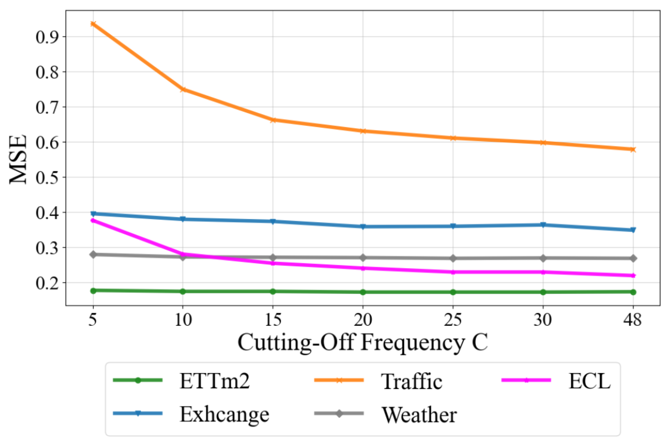
4.3.4. Cutting-Off Frequency

This experiment explores the relationship of the cutting-off frequency C with prediction performance and space consumption. In our approach, the cropping frequency is obtained by multiplying the hyper-parameter $\eta$ and the length of the input sequence. In mainstream experiments, the input sequence is uniformly 96, so for intuition, we directly use the cutting-off frequency C as the experimental variable. A smaller cropping frequency means that more low-frequency information is retained and more high-frequency information is discarded. An increase in the cutting-off frequency C means that the frequency domain component information is preserved more comprehensively.

As shown in Figure 7, there is an overall trend of better prediction as the cutting-off frequency C increases. However, different datasets exhibit a large gap in performance growth and a large gap in the role of different frequency domain components. For example, the Traffic dataset shows a rapid decrease in MSE at first as the cutting-off frequency C grows, and after a C of 20, this slows down. This suggests that the low-frequency component is very important in this dataset, while the high-frequency component is not as effective in terms of the information it contains. Similarly, the ECL dataset has a similar pattern. The Exchange dataset, on the other hand, exhibits a rapid decline in the mid-frequency part, showing a more significant importance compared to the low-frequency and high-frequency parts. In contrast, the ETTm2 and Weather datasets show very little change as the cutting-off frequency C grows.

Figure 7. Correlation analysis of cutting-off frequency with predicted performance on five datasets.

Table 5 shows the more comprehensive and detailed data and the corresponding parameter count occupancy. Further reflecting the differences among the datasets, it suggests that scenario differences should be fully considered when deploying towards applications, striving for a more convenient and efficient model while guaranteeing the prediction results.

Table 5. Predictive performance of seven cutting-off frequencies on eight datasets with corresponding number of parameters (NOP). The best performance at each setting is shown by the bolding.

CutFreq C Metric		5	10	15	20	25	30	48
		MSE	MSE	MSE	MSE	MSE	MSE	MSE
ETTm1	Avg	0.511	0.489	0.493	0.486	0.488	0.488	0.484
ETTm2	Avg	0.177	0.174	0.174	0.172	0.172	0.172	0.173
ETTh1	Avg	0.675	0.582	0.572	0.570	0.559	0.577	0.575
ETTh2	Avg	0.251	0.248	0.243	0.244	0.244	0.240	0.241
ECL	Avg	0.376	0.280	0.254	0.240	0.229	0.229	0.219
Exchange	Avg	0.395	0.379	0.373	0.358	0.359	0.363	0.348
Traffic	Avg	0.935	0.749	0.662	0.630	0.610	0.597	0.578
Weather	Avg	0.279	0.272	0.271	0.270	0.268	0.269	0.268
1st Count		0	0	0	1	3	2	5
NOP (K)		4.20	9.3	15.43	22.63	30.85	40.16	82.29

4.3.5. Input Length

This experiment explores the correlation of input sequence length with prediction performance. It has been shown that the transformer-based points-oriented approach is limited by being naturally permutation-invariant and anti-ordering, such that the prediction performance does not improve as the input sequence length grows [19]. Whereas, in our variables-oriented frequency-wise method, more frequency components are added as the input sequence length grows, leading to greater information capacity.

As shown in Figure 8, overall, as the input length grows, the MSE decreases dramatically and the prediction accuracy improves significantly, demonstrating the ability of our method to extract complex time-dependent relationships from longer inputs. This is especially the case for the Traffic dataset and the ECL dataset. This demonstrates that the frequency components of these two datasets demand more than just inputs of length 96. Longer inputs result in richer feature details that rely on our model for modeling analysis. In contrast, the Exchange dataset at 192 and 384 inputs instead slightly reduces the prediction performance. This may be related to the fact that this dataset has uniquely irregular high-frequency noise.

Figure 8. Correlation analysis of input length with predicted performance. The scores are averaged over the dataset for the four prediction lengths: 96, 192, 336, 720. The parameter occupancy of the model is demonstrated after the input length of the sequence. The blue dashed line shows the trend in the traffic dataset. The black dashed line shows the trend in the Exchange dataset. The red dashed line shows the trend in the ECL dataset.

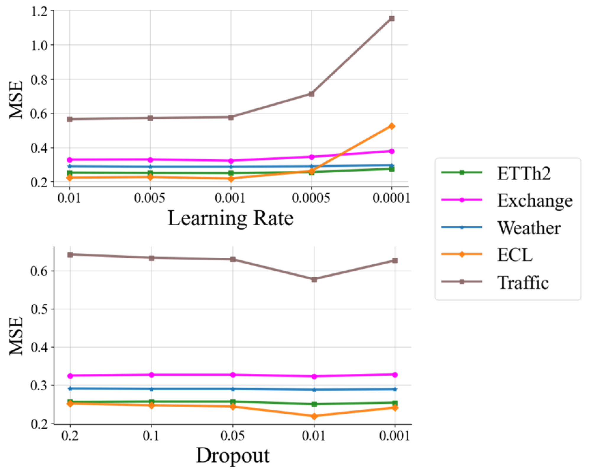
4.3.6. Hyper-Parameter Sensitivity

As shown in Figure 9, the hyper-parameter sensitivity experiments on learning rate and dropout demonstrate the flexibility of our approach. Changes in both within a reasonable range do not affect the prediction results or cause drastic shifts in the metrics. Most of the differences are within acceptable limits. Only the impact of too low an initial learning rate is significant; too low a learning rate implies underfitting, which makes the predictions significantly worse.

Figure 9. The Effect of Learning Rate and Dropout on Model Training.

5. Conclusions

We propose a frequency-wise and variables-oriented transformer-based multivariate time series prediction method. From the perspective of frequency-wise multi-representation, we propose frequency-enhanced block and frequency-enhanced independent representation multi-head attention. Among them, cutting-off frequency is used to remove the high-frequency noise of the sequence and combined with equivalent mapping to make the model lightweight overall. The independent sub-head strategy ensures that the amplitude, phase, and real and imaginary parts do not interfere with each other in completing the multivariate correlation construction, thus fully capturing the dependence of the frequency components of the variables. Subsequently, down-sampling of the multi-representation obeys the global perspective to blend the information, while the complex-valued linear layer utilises complex multiplication for accurate interpolation mapping. The experiments demonstrate the effectiveness and efficiency of the proposed method to achieve top-tier prediction performance with remarkably small temporal and spatial consumption. The experiments further analyze the role and contribution of the frequency domain representations and the necessity of independent mapping as well as demonstrating the trade-offs between performance and efficiency of cutting-off frequency and equivalent mapping. Overall, our frequency-enhanced transformer with lightweight multi-representation provides a novel network design perspective based on the frequency domain, providing deeper insight into multivariate time series, which is an important innovation in the field of time series analysis.

References

1. Yasar, H.; Kilimci, Z.H. US dollar/Turkish lira exchange rate forecasting model based on deep learning methodologies and time series analysis. Symmetry 2020, 12, 1553. [Google Scholar] [CrossRef]
2. Alyousifi, Y.; Othman, M.; Sokkalingam, R.; Faye, I.; Silva, P.C. Predicting daily air pollution index based on fuzzy time series markov chain model. Symmetry 2020, 12, 293. [Google Scholar] [CrossRef]
3. Cruz-Nájera, M.A.; Treviño-Berrones, M.G.; Ponce-Flores, M.P.; Terán-Villanueva, J.D.; Castán-Rocha, J.A.; Ibarra-Martínez, S.; Santiago, A.; Laria-Menchaca, J. Short time series forecasting: Recommended methods and techniques. Symmetry 2022, 14, 1231. [Google Scholar] [CrossRef]
4. Kambale, W.V.; Salem, M.; Benarbia, T.; Al Machot, F.; Kyamakya, K. Comprehensive Sensitivity Analysis Framework for Transfer Learning Performance Assessment for Time Series Forecasting: Basic Concepts and Selected Case Studies. Symmetry 2024, 16, 241. [Google Scholar] [CrossRef]
5. Lara-Benítez, P.; Carranza-García, M.; Luna-Romera, J.M.; Riquelme, J.C. Temporal convolutional networks applied to energy-related time series forecasting. Appl. Sci. 2020, 10, 2322. [Google Scholar] [CrossRef]
6. Das, M.; Ghosh, S.K. semBnet: A semantic Bayesian network for multivariate prediction of meteorological time series data. Pattern Recognit. Lett. 2017, 93, 192–201. [Google Scholar] [CrossRef]
7. Shering, T.; Alonso, E.; Apostolopoulou, D. Investigation of Load, Solar and Wind Generation as Target Variables in LSTM Time Series Forecasting, Using Exogenous Weather Variables. Energies 2024, 17, 1827. [Google Scholar] [CrossRef]
8. Martínez-Álvarez, F.; Troncoso, A.; Asencio-Cortés, G.; Riquelme, J.C. A survey on data mining techniques applied to electricity-related time series forecasting. Energies 2015, 8, 13162–13193. [Google Scholar] [CrossRef]
9. Chan, S.; Oktavianti, I.; Puspita, V. A deep learning CNN and AI-tuned SVM for electricity consumption forecasting: Multivariate time series data. In Proceedings of the 2019 IEEE 10th Annual Information Technology, Electronics and Mobile Communication Conference (IEMCON), Vancouver, BC, Canada, 7–19 October 2019; IEEE: Piscataway, NJ, USA, 2019; pp. 488–494. [Google Scholar]
10. Ghosh, B.; Basu, B.; O’Mahony, M. Multivariate short-term traffic flow forecasting using time-series analysis. IEEE Trans. Intell. Transp. Syst. 2009, 10, 246–254. [Google Scholar] [CrossRef]
11. Shah, I.; Muhammad, I.; Ali, S.; Ahmed, S.; Almazah, M.M.; Al-Rezami, A. Forecasting day-ahead traffic flow using functional time series approach. Mathematics 2022, 10, 4279. [Google Scholar] [CrossRef]
12. He, K.; Yang, Q.; Ji, L.; Pan, J.; Zou, Y. Financial time series forecasting with the deep learning ensemble model. Mathematics 2023, 11, 1054. [Google Scholar] [CrossRef]
13. Niu, T.; Wang, J.; Lu, H.; Yang, W.; Du, P. Developing a deep learning framework with two-stage feature selection for multivariate financial time series forecasting. Expert Syst. Appl. 2020, 148, 113237. [Google Scholar] [CrossRef]
14. Liu, Z.; Zhu, Z.; Gao, J.; Xu, C. Forecast methods for time series data: A survey. IEEE Access 2021, 9, 91896–91912. [Google Scholar] [CrossRef]
15. Chen, Z.; Ma, M.; Li, T.; Wang, H.; Li, C. Long sequence time-series forecasting with deep learning: A survey. Inf. Fusion 2023, 97, 101819. [Google Scholar] [CrossRef]
16. Ahmed, S.; Nielsen, I.E.; Tripathi, A.; Siddiqui, S.; Ramachandran, R.P.; Rasool, G. Transformers in time-series analysis: A tutorial. Circuits Syst. Signal Process. 2023, 42, 7433–7466. [Google Scholar] [CrossRef]
17. Zhou, H.; Zhang, S.; Peng, J.; Zhang, S.; Li, J.; Xiong, H.; Zhang, W. Informer: Beyond efficient transformer for long sequence time-series forecasting. Proc. AAAI Conf. Artif. Intell. 2021, 35, 11106–11115. [Google Scholar] [CrossRef]
18. Zhou, T.; Ma, Z.; Wen, Q.; Wang, X.; Sun, L.; Jin, R. Fedformer: Frequency enhanced decomposed transformer for long-term series forecasting. In Proceedings of the 39th International Conference on Machine Learning, Baltimore, MD, USA, 17–23 July 2022; pp. 27268–27286. [Google Scholar]
19. Zeng, A.; Chen, M.; Zhang, L.; Xu, Q. Are transformers effective for time series forecasting? Proc. AAAI Conf. Artif. Intell. 2023, 37, 11121–11128. [Google Scholar] [CrossRef]
20. Liu, Y.; Hu, T.; Zhang, H.; Wu, H.; Wang, S.; Ma, L.; Long, M. iTransformer: Inverted Transformers Are Effective for Time Series Forecasting. arXiv 2023, arXiv:2310.06625. [Google Scholar]
21. Valipour, M.; Banihabib, M.E.; Behbahani, S.M.R. Comparison of the ARMA, ARIMA, and the autoregressive artificial neural network models in forecasting the monthly inflow of Dez dam reservoir. J. Hydrol. 2013, 476, 433–441. [Google Scholar] [CrossRef]
22. Sapankevych, N.I.; Sankar, R. Time series prediction using support vector machines: A survey. IEEE Comput. Intell. Mag. 2009, 4, 24–38. [Google Scholar] [CrossRef]
23. Parmezan, A.R.S.; Souza, V.M.; Batista, G.E. Evaluation of statistical and machine learning models for time series prediction: Identifying the state-of-the-art and the best conditions for the use of each model. Inf. Sci. 2019, 484, 302–337. [Google Scholar] [CrossRef]
24. Bontempi, G.; Ben Taieb, S.; Le Borgne, Y.A. Machine learning strategies for time series forecasting. In Proceedings of the Business Intelligence: Second European Summer School, eBISS 2012, Tutorial Lectures 2, Brussels, Belgium, 15–21 July 2013; pp. 62–77. [Google Scholar]
25. Han, Z.; Zhao, J.; Leung, H.; Ma, K.F.; Wang, W. A review of deep learning models for time series prediction. IEEE Sens. J. 2019, 21, 7833–7848. [Google Scholar] [CrossRef]
26. Mandal, A.K.; Sen, R.; Goswami, S.; Chakraborty, B. Comparative study of univariate and multivariate long short-term memory for very short-term forecasting of global horizontal irradiance. Symmetry 2021, 13, 1544. [Google Scholar] [CrossRef]
27. Zhao, Z.; Chen, W.; Wu, X.; Chen, P.C.; Liu, J. LSTM network: A deep learning approach for short-term traffic forecast. IET Intell. Transp. Syst. 2017, 11, 68–75. [Google Scholar] [CrossRef]
28. Lai, G.; Chang, W.C.; Yang, Y.; Liu, H. Modeling long-and short-term temporal patterns with deep neural networks. In Proceedings of the 41st International ACM SIGIR Conference on Research & Development in Information Retrieval, Ann Arbor, MI, USA, 8–12 July 2018; pp. 95–104. [Google Scholar]
29. Almuammar, M.; Fasli, M. Deep learning for non-stationary multivariate time series forecasting. In Proceedings of the 2019 IEEE International Conference on Big Data (Big Data), Angeles, CA, USA, 9–12 December 2019; IEEE: Piscataway, NJ, USA, 2019; pp. 2097–2106. [Google Scholar]
30. Saini, U.; Kumar, R.; Jain, V.; Krishnajith, M. Univariant Time Series forecasting of Agriculture load by using LSTM and GRU RNNs. In Proceedings of the 2020 IEEE Students Conference on Engineering & Systems (SCES), Prayagraj, India, 10–12 July 2020; IEEE: Piscataway, NJ, USA, 2020; pp. 1–6. [Google Scholar]
31. Torres, J.F.; Hadjout, D.; Sebaa, A.; Martínez-Álvarez, F.; Troncoso, A. Deep learning for time series forecasting: A survey. Big Data 2021, 9, 3–21. [Google Scholar] [CrossRef]
32. O’Shea, K.; Nash, R. An introduction to convolutional neural networks. arXiv 2015, arXiv:1511.08458. [Google Scholar]
33. Bai, S.; Kolter, J.Z.; Koltun, V. An empirical evaluation of generic convolutional and recurrent networks for sequence modeling. arXiv 2018, arXiv:1803.01271. [Google Scholar]
34. Lim, B.; Zohren, S. Time-series forecasting with deep learning: A survey. Philos. Trans. R. Soc. A 2021, 379, 20200209. [Google Scholar] [CrossRef]
35. Wen, Q.; Zhou, T.; Zhang, C.; Chen, W.; Ma, Z.; Yan, J.; Sun, L. Transformers in time series: A survey. arXiv 2022, arXiv:2202.07125. [Google Scholar]
36. Benidis, K.; Rangapuram, S.S.; Flunkert, V.; Wang, Y.; Maddix, D.; Turkmen, C.; Gasthaus, J.; Bohlke-Schneider, M.; Salinas, D.; Stella, L.; et al. Deep learning for time series forecasting: Tutorial and literature survey. ACM Comput. Surv. 2022, 55, 1–36. [Google Scholar] [CrossRef]
37. Miller, J.A.; Aldosari, M.; Saeed, F.; Barna, N.H.; Rana, S.; Arpinar, I.B.; Liu, N. A survey of deep learning and foundation models for time series forecasting. arXiv 2024, arXiv:2401.13912. [Google Scholar]
38. Liu, Z.; Lin, Y.; Cao, Y.; Hu, H.; Wei, Y.; Zhang, Z.; Lin, S.; Guo, B. Swin transformer: Hierarchical vision transformer using shifted windows. In Proceedings of the IEEE/CVF International Conference on Computer Vision, Montreal, QC, Canada, 10–17 October 2021; pp. 10012–10022. [Google Scholar]
39. Vaswani, A.; Shazeer, N.; Parmar, N.; Uszkoreit, J.; Jones, L.; Gomez, A.N.; Kaiser, Ł.; Polosukhin, I. Attention is all you need. Adv. Neural Inf. Process. Syst. 2017, 30. [Google Scholar]
40. Shih, S.Y.; Sun, F.K.; Lee, H.Y. Temporal pattern attention for multivariate time series forecasting. Mach. Learn. 2019, 108, 1421–1441. [Google Scholar] [CrossRef]
41. Beltagy, I.; Peters, M.E.; Cohan, A. Longformer: The long-document transformer. arXiv 2020, arXiv:2004.05150. [Google Scholar]
42. Wang, S.; Li, B.Z.; Khabsa, M.; Fang, H.; Ma, H. Linformer: Self-attention with linear complexity. arXiv 2020, arXiv:2006.04768. [Google Scholar]
43. Li, S.; Jin, X.; Xuan, Y.; Zhou, X.; Chen, W.; Wang, Y.X.; Yan, X. Enhancing the locality and breaking the memory bottleneck of transformer on time series forecasting. Adv. Neural Inf. Process. Syst. 2019, 32. [Google Scholar]
44. Liu, S.; Yu, H.; Liao, C.; Li, J.; Lin, W.; Liu, A.X.; Dustdar, S. Pyraformer: Low-complexity pyramidal attention for long-range time series modeling and forecasting. In Proceedings of the International Conference on Learning Representations, Virtual Event, 3–7 May 2021. [Google Scholar]
45. Wu, H.; Xu, J.; Wang, J.; Long, M. Autoformer: Decomposition transformers with auto-correlation for long-term series forecasting. Adv. Neural Inf. Process. Syst. 2021, 34, 22419–22430. [Google Scholar]
46. Du, D.; Su, B.; Wei, Z. Preformer: Predictive transformer with multi-scale segment-wise correlations for long-term time series forecasting. In Proceedings of the ICASSP 2023—2023 IEEE International Conference on Acoustics, Speech and Signal Processing (ICASSP), Rhodes Island, Greece, 4–10 June 2023; IEEE: Piscataway, NJ, USA, 2023; pp. 1–5. [Google Scholar]
47. Lee-Thorp, J.; Ainslie, J.; Eckstein, I.; Ontanon, S. Fnet: Mixing tokens with fourier transforms. arXiv 2021, arXiv:2105.03824. [Google Scholar]
48. Wu, H.; Hu, T.; Liu, Y.; Zhou, H.; Wang, J.; Long, M. Timesnet: Temporal 2d-variation modeling for general time series analysis. In Proceedings of the The Eleventh International Conference on Learning Representations, Vienna, Austria, 7–11 May 2022. [Google Scholar]
49. Xu, Z.; Zeng, A.; Xu, Q. FITS: Modeling Time Series with 10 k Parameters. arXiv 2023, arXiv:2307.03756. [Google Scholar]
50. Zhou, T.; Ma, Z.; Wen, Q.; Sun, L.; Yao, T.; Yin, W.; Jin, R. Film: Frequency improved legendre memory model for long-term time series forecasting. Adv. Neural Inf. Process. Syst. 2022, 35, 12677–12690. [Google Scholar]
51. Rosenblatt, F. The perceptron: A probabilistic model for information storage and organization in the brain. Psychol. Rev. 1958, 65, 386. [Google Scholar] [CrossRef] [PubMed]
52. Bridle, J.S. Probabilistic interpretation of feedforward classification network outputs, with relationships to statistical pattern recognition. In Neurocomputing: Algorithms, Architectures and Applications; Springer: Berlin/Heidelberg, Germany, 1990; pp. 227–236. [Google Scholar]
53. Liu, M.; Zeng, A.; Chen, M.; Xu, Z.; Lai, Q.; Ma, L.; Xu, Q. Scinet: Time series modeling and forecasting with sample convolution and interaction. Adv. Neural Inf. Process. Syst. 2022, 35, 5816–5828. [Google Scholar]
54. Das, A.; Kong, W.; Leach, A.; Sen, R.; Yu, R. Long-term forecasting with tide: Time-series dense encoder. arXiv 2023, arXiv:2304.08424. [Google Scholar]
55. Paszke, A.; Gross, S.; Massa, F.; Lerer, A.; Bradbury, J.; Chanan, G.; Killeen, T.; Lin, Z.; Gimelshein, N.; Antiga, L.; et al. Pytorch: An imperative style, high-performance deep learning library. Adv. Neural Inf. Process. Syst. 2019, 32. [Google Scholar]
56. Adam, K.D.B.J. A method for stochastic optimization. arXiv 2014, arXiv:1412.6980. [Google Scholar]
Disclaimer/Publisher’s Note: The statements, opinions and data contained in all publications are solely those of the individual author(s) and contributor(s) and not of MDPI and/or the editor(s). MDPI and/or the editor(s) disclaim responsibility for any injury to people or property resulting from any ideas, methods, instructions or products referred to in the content.
Article Metrics
Citations
Article Access Statistics
Multiple requests from the same IP address are counted as one view.