Abstract
The Tree-Seed Algorithm (TSA) has been effective in addressing a multitude of optimization issues. However, it has faced challenges with early convergence and difficulties in managing high-dimensional, intricate optimization problems. To tackle these shortcomings, this paper introduces a TSA variant (DTSA). DTSA incorporates a suite of methodological enhancements that significantly bolster TSA’s capabilities. It introduces the PSO-inspired seed generation mechanism, which draws inspiration from Particle Swarm Optimization (PSO) to integrate velocity vectors, thereby enhancing the algorithm’s ability to explore and exploit solution spaces. Moreover, DTSA’s adaptive velocity adaptation mechanism based on count parameters employs a counter to dynamically adjust these velocity vectors, effectively curbing the risk of premature convergence and strategically reversing vectors to evade local optima. DTSA also integrates the trees population integrated evolutionary strategy, which leverages arithmetic crossover and natural selection to bolster population diversity, accelerate convergence, and improve solution accuracy. Through experimental validation on the IEEE CEC 2014 benchmark functions, DTSA has demonstrated its enhanced performance, outperforming recent TSA variants like STSA, EST-TSA, fb-TSA, and MTSA, as well as established benchmark algorithms such as GWO, PSO, BOA, GA, and RSA. In addition, the study analyzed the best value, mean, and standard deviation to demonstrate the algorithm’s efficiency and stability in handling complex optimization issues, and DTSA’s robustness and efficiency are proven through its successful application in five complex, constrained engineering scenarios, demonstrating its superiority over the traditional TSA by dynamically optimizing solutions and overcoming inherent limitations.
1. Introduction
An optimization problem involves the pursuit of the optimal or an approximate optimal solution within prescribed constraints [1]. This typically necessitates identifying variable values that either maximize or minimize a specific objective function [2,3]. Such problems are fundamental in scientific inquiry, engineering, and various other disciplines, driving advancements in diverse fields through systematic problem-solving approaches [4,5,6]. However, when solving optimization problems in the real world, we encounter countless complexities, including high computational requirements, nonlinear constraints, dynamic or noisy objective functions, etc. [7]. These challenges significantly impact the decision-making process for selecting the appropriate optimization algorithms. Against this backdrop, exact algorithms provide precise global optimum solutions. However, as the number of variables increases, their execution time grows exponentially. This exponential growth makes them impractical for large-scale or highly complex scenarios [8]. Therefore, stochastic optimization algorithms, especially heuristic and metaheuristic algorithms within the realm of approximate solutions, emerge as practical tools for tackling complex issues [9,10].
Heuristic and metaheuristic algorithms are favored for their ability to search for optimal or near-optimal solutions within a reasonable timeframe by employing probabilistic and statistical methods [11,12]. These algorithms are particularly suited for addressing complex problems that are beyond the reach of traditional methods. On the one hand, heuristics utilize problem-specific strategies, relying on intuitive logic to make decisions that guide the search process towards promising areas of the solution space [13,14]. On the other hand, metaheuristics provide a higher level of abstraction, offering a framework adaptable to various optimization problems without the need for customization to a specific issue [15]. This shift towards heuristic and metaheuristic algorithms represents a natural response to the limitations of exact algorithms, underscoring their significance in solving the complex optimization challenges characteristic of many real-world applications [6,16,17].
As depicted in Figure 1, metaheuristic algorithms can be broadly categorized as non-nature-inspired or nature-inspired. Examples of non-nature-inspired algorithms include Tabu Search (TS) [18,19], Iterated Local Search (ILS) [20,21], and Adaptive Dimensional Search (ADS) [22], many algorithms draw inspiration from natural phenomena. Nature-inspired algorithms, such as Differential Evolution (DE) [23,24], Particle Swarm Optimization (PSO) [25,26], Artificial Bee Colony (ABC) [27,28], Krill Herd (KH) [29,30], and Gravitational Search Algorithm (GSA) [31,32], are valued for their versatility and simplicity in tackling complex optimization challenges [23]. However, it is essential to note that while some algorithms excel in addressing specific problems, their effectiveness may vary across different or intricate scenarios [33].
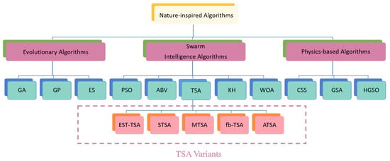
Figure 1.
The classification of nature-inspired algorithms.
Among them, the Tree-Seed Algorithm (TSA) stands out as a successful nature-inspired metaheuristic developed in 2015, drawing inspiration from the natural interplay between tree and seed evolution [34]. TSA approaches optimization problems by exploring the locations of trees and seeds, representing feasible solutions [35,36]. Notably, TSA has gained widespread adoption, surpassing some swarm intelligence algorithms in popularity due to its simpler structure, higher precision, and greater robustness [37]. Nevertheless, TSA exhibits drawbacks, including premature convergence and a susceptibility to stagnate in local optima [38]. This study aims to mitigate these issues through novel approaches, including a distinct initial design and algorithmic modifications and hybridizations.
1.1. Motivations
TSA is a population-based approach to evolution that takes its inspiration from the relationship between trees and seeds, which are spread to the ground for reproduction. TSA is simple, has few parameters, it is easy to understand the concept, and it is effective in solving continuous structure optimization problems [34]. However, the TSA has its limits. During space exploration, it is often trapped in a locally optimal solution, struggling to escape this mechanism [39]. In addition, the optimal solutions generated for each round are underutilized, resulting in a relatively single optimal position [40]. These shortcomings highlight the need to refine the TSA methodology to improve its effectiveness and extend its applicability to optimization tasks. However, it is these shortcomings that motivate us to improve it. The motivations driving this research are as follows:
- The existing seed generation mechanism in TSA lacks consideration of population attributes and may lead to seeds being generated in less favorable regions of the search space [41]. By redesigning the tree selection process, we aim to improve the quality of generated seeds and enhance the algorithm’s overall performance.
- In the TSA evolutionary process, interactions solely between trees and seeds ignore potential interactions among trees, reducing population diversity [42]. To tackle this, we propose a tree population strategy to boost diversity and speed up convergence.
- Many optimization algorithms rely on simplistic initialization methods, such as uniform random sampling, which may result in a less diverse initial population [43]. By rethinking the initialization process, we aim to improve the exploration–exploitation balance and enhance the algorithm’s robustness across various optimization scenarios.
1.2. Contribution
The no free lunch (NFL) theorem holds significance within this context [44]. This study is notably driven by the explicit goal of reducing the probability of conventional TSA encountering stagnation in local optima and premature convergence. This study aims to enhance the balance between exploitation and exploration by incorporating the PSO velocity update mechanism and an improved balance mechanism into the original TSA. The primary contributions of this paper can be succinctly summarized as follows.
- PSO-Inspired seed generation mechanism: The significant advancement of this TSA variant lies in its seed generation technique, which is inspired by PSO. By utilizing velocity vectors for updating seed positions, this approach introduces a dynamic and adaptive element to the exploration–exploitation equilibrium, thereby augmenting the algorithm’s efficacy in traversing the search space efficiently.
- Adaptive dynamic parameter update mechanism: The incorporation of adaptive weight (w) and constant (k) updates during the optimization process is a novel aspect. This adaptive mechanism allows the algorithm to dynamically adjust its exploration and exploitation tendencies based on the current iteration, contributing to improved convergence behavior and solution quality.
- Adaptive velocity adaptation mechanism based on count parameters: The introduction of a count-based adaptive mechanism for updating the velocity vectors contributes to the algorithm’s ability to dynamically adjust its behavior during different phases of the optimization process. The count parameter influences the exploration–exploitation trade-off, allowing the algorithm to adapt its strategy as the optimization progresses.
- Population-based evolutionary strategy with information exchange: The variant integrates an evolutionary strategy characterized by dynamic partitioning of the population into distinct subpopulations based on their respective fitness values. This innovative approach incorporates a combination of grouping, crossover, and natural selection operations. Crossover events are facilitated between the superior subpopulation and a subset of the inferior subpopulation, facilitating structured information exchange. Concurrently, a natural selection operation replaces the inferior subpopulation with the superior counterpart in terms of both position and velocity. This sophisticated methodology enhances the algorithm’s adaptability, facilitating the effective exploitation of promising solutions while concurrently preserving population diversity to mitigate premature convergence.
- Dynamic seeding with chaotic map: The sine chaotic map is used for generating random numbers during the initialization phase and seed production [45]. Chaotic maps can provide a better and more dynamic exploration of the search space compared to uniform random numbers. This can enhance the diversity of the seeds produced and potentially improve the algorithm’s ability to escape from local optima.
2. Related Work
2.1. A Brief Introduction to TSA
The TSA, proposed by Mustafa Servet Kiran in 2015, is a swarm intelligence algorithm inspired by the relationship between trees and seeds on land [34]. TSA is designed for solving continuous optimization problems and is widely applicable in heuristic and population-based search scenarios. The key principles of TSA are outlined below:
- Tree position initialization: The initial position of each tree () is determined by randomly selecting values for each dimension (j) within the specified bounds of the search space, using Equation (1).where is the j-th dimension of the i-th tree, and are the lower and upper bounds of the search space for dimension j, and is a random number in the range of .
- Tree-seed renewal mechanism: The seed renewal mechanism involves two update formulas for generating new seeds, considering both the current tree’s location and the optimal location of the entire tree population, which are calculated in Equations (2) and (3).where is the j-th dimension of the seed to be produced by the i-th tree, is the j-th dimension of the i-th tree, is the j-th dimension of the best tree location obtained so far, is the j-th dimension of a randomly selected tree (r) from the population, and is a scaling factor randomly generated in the range .
2.2. Literature Review
The TSA has gained significant attention in the swarm intelligence research community. It has become widely adopted due to its simplicity, precision, and robustness in comparison to other swarm intelligence algorithms [46]. Researchers have continuously proposed variants to improve TSA’s performance, with a focus on enhancing seed generation, tree migration, and expanding its application domains [35].
- Tree migration variants: The Migration Tree-Seed Algorithm (MTSA) incorporates hierarchical gravity learning and random-based migration, drawing inspiration from the Grey Wolf Optimizer [38]. This approach effectively mitigates challenges related to exploration–exploitation imbalance, local stagnation, and premature convergence. Additionally, the Triple Tree-Seed Algorithm (TriTSA) introduces triple learning-based mechanisms, amalgamating migration strategies with sine random distribution to further enhance algorithmic performance [47].
- Innovations in seed generation: Various innovations have emerged to enhance seed generation and improve the effectiveness of the optimization process. Jiang’s integration of the Sine Cosine Algorithm (SCA) with TSASC introduces a novel mechanism for updating seed positions, refining weight factors to pursue optimal solutions [48]. Additionally, the Sine Tree-Seed Algorithm (STSA) dynamically adjusts seed quantity, transitioning from higher to lower counts to emphasize output bolstering during initial search phases [42]. Other TSA variants like ITSA, incorporating an acceleration coefficient for faster updates [49], and EST-TSA, leveraging the current optimal population position for improved local search, make significant contributions [50]. Innovations such as fb-TSA [51], integrating seeds and search tendencies via feedback mechanisms [51], and LTSA, introducing a Lévy flight random walk strategy to seed position equations [52], collectively refine TSA’s performance and adaptability in optimization tasks.
- Algorithm applications: TSA and its various iterations are applied across a wide array of fields. For instance, CTSA is adept at handling constrained optimization problems by leveraging Deb’s rules for tree and seed selection [53]. Meanwhile, DTSA integrates swap, shift, and symmetry transformation operators to tackle permutation-coded optimization problems [54]. In financial risk assessment, Jiang introduces the sinhTSA-MLP model for identifying credit default risks with remarkable precision [55]. Moreover, in the medical domain, Aslan proposes the TSA-ANN structure for precise COVID-19 diagnosis, optimizing artificial neural networks to classify deep architectural features [56].
The broad range of applications demonstrates the adaptability and efficacy of TSA and its derivatives in tackling multifaceted challenges spanning various domains. Continuous improvements and fine-tuning bolster TSA’s optimization prowess, solidifying its role as a pivotal tool in diverse problem-solving contexts.
2.3. An Overview of PSO
PSO is a popular metaheuristic algorithm designed for solving global optimization problems. Proposed by Dr. Eberhart and Dr. Kennedy in 1995, PSO draws inspiration from the social behavior of bird flocks and fish schools [57]. The working principle of the PSO algorithm can be briefly summarized as follows.
In the initialization phase, particles are randomly generated within the search space. Each particle is characterized by its position and velocity , where D denotes the problem’s dimensionality and i is the index of the particle. Next, the fitness of each particle is evaluated by applying the objective function to its current position by Equation (4).
Subsequently, the local best position () for each particle and the global best position () for the entire swarm are updated based on fitness improvement, as shown in Equation (5) below:
Then, the particle velocities and positions are updated using the velocity and position update formulas, considering inertia (w), cognitive (), and social () components, as shown below in Equation (6):
where w is the inertia weight, and are learning rates, and and are random numbers between 0 and 1. Finally, through iterative optimization, the swarm converges towards the global optimum or an approximate solution.
3. Methods
3.1. PSO-Inspired Seed Generation Mechanism
The original TSA employed a rudimentary seed generation mechanism based on random perturbations of tree positions within the search space. This approach lacked a systematic and adaptive strategy, which could lead to suboptimal exploration and exploitation. To address these limitations, we introduce a novel PSO-inspired seed generation mechanism; in this mechanism, each tree has a certain initial velocity. Furthermore, in the process of generating seeds, the velocity update of each tree is also affected by ST. As a result, two update strategies emerge: the speed update strategy for local development and the speed update strategy for global development, as depicted in Equation (9) and illustrated in Figure 2. These strategies introduce a dynamic and adaptive element to speed generation, as detailed in Equation (8) and demonstrated in Figure 3.
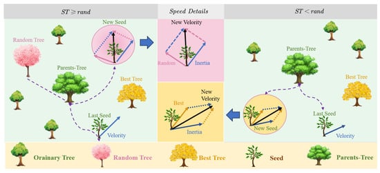
Figure 2.
The principle of velocity-driven seed generation.
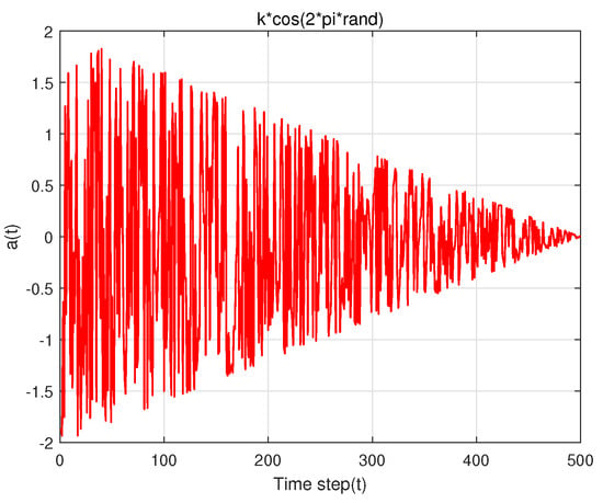
Figure 3.
The variation in k * cos (2 * pi * rand) with the number of iterations.
In the speed vector update mechanism of seeds, represents the inertia or influence of the previous velocity on the current velocity. The inertia weight (w) ensures that the algorithm retains some information from the previous iteration, contributing to the smooth transition between consecutive velocities and aiding in the stability of the optimization process. introduces a random perturbation to the velocity, facilitating exploration of the solution space. The subtraction signifies the difference in positions between the current tree (i) and a randomly chosen neighboring tree (r). Multiplying by introduces a random scaling factor, adding stochasticity to the algorithm. utilizes k as a control parameter to adjust the amplitude of the cosine term. The cosine function introduces periodicity and oscillatory behavior to the velocity update, aiding exploration by allowing the algorithm to escape local optima and explore diverse regions of the solution space. Multiplying by k provides adaptive control over the amplitude of the cosine term.
Meanwhile, the updated speed will be incorporated into Equations (2) and (3), as described in Equation (9), utilizing velocity vector integration to update the seed position. The introduction of velocity vectors in the optimization process is pivotal for enhancing the exploration–exploitation balance and adaptability of the algorithm by integrating velocity vectors for updating seed positions.
3.2. Adaptive Velocity Adaptation Mechanism Based on Count Parameters
The static nature of TSA, with a fixed velocity update strategy, limits its adaptability across various optimization scenarios, leading to issues such as premature convergence and insufficient exploration. The introduced count-based adaptive mechanism dynamically adjusts the algorithm’s behavior, effectively balancing exploration and exploitation. A pivotal enhancement is introduced through the incorporation of a counter, denoted as count, to monitor changes in the global optimal tree. If the global optimal tree is replaced, the counter resets to zero. Conversely, if the global optimal tree remains unchanged for a consecutive duration, when the count reaches a threshold of 15, it indicates being trapped in a local optimum. To overcome this challenge and facilitate escape from local optima, the velocity vector is inverted (Equation (10) and Figure 4). This inversion disrupts the pattern leading to local optima, enabling seeds to break free from suboptimal solutions. This innovative approach significantly bolsters the algorithm’s global search capability by promoting diversity and exploration, enhancing resilience against convergence to suboptimal solutions.
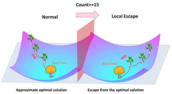
Figure 4.
Adaptive velocity adaptation mechanism based on count parameters.
3.3. Population-Based Evolutionary Strategy with Information Exchange Mechanism
Due to the standard TSA’s slow convergence speed and diminished population diversity in later iterations, achieving the global optimal value becomes challenging. To address this, arithmetic crossover and natural selection strategies are incorporated to enhance tree diversity, convergence speed, and accuracy illustrated in Figure 5. The trees are arranged by selecting the absolute values of all particle fitness values, as shown in Equation (11), and divided according to Equation (12).
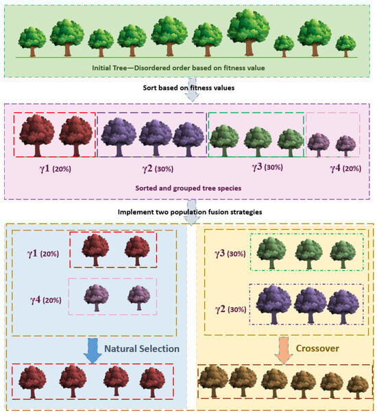
Figure 5.
Schematic of population-based evolutionary strategy with information exchange.
In Equation (12), the fitness values are partitioned into four components: , , , and . The stochastic nature of the TSA algorithm categorizes fitness values into two groups: favorable () and unfavorable (). Specifically, and each constitute 20% of the total population, while and each represent 30%.
The crossover operation is applied to and , facilitating the fusion of trees with favorable and unfavorable fitness values. This approach generates offspring with increased diversity and propels less fit trees towards improved fitness values.
Simultaneously, natural selection acts upon and . This process involves directly replacing the velocity and position of less fit trees () with those of more fit trees (), analogous to reducing the entire population by 20%, significantly accelerating the convergence speed of particles.
The specific strategies are as follows:
- Arithmetic crossover: This paper proposes a novel crossover strategy for trees based on the crossover strategy of Differential Evolution (DE). The update equations for the position and velocity of trees at the locations and , respectively, are defined as follows:where , , , and represent the positions and velocities of trees, as defined in Equations (11) and (12), and rand is a random number uniformly distributed in the range [0, 1].
- Natural selection: To expedite the convergence speed of trees, a mechanism is employed whereby well-performing trees replace less effective ones. The procedure is expressed as Equations (17) and (18):where , , , and represent the positions and velocities of trees as defined in Equation (12). This natural selection process involves the direct replacement of the position and velocity of less effective trees () with those of more effective trees (), significantly accelerating the convergence of trees.
3.4. DTSA: A Novel Tree-Seed Algorithm
The proposed algorithm represents a substantial improvement over the original TSA by addressing its limitations through a multifaceted approach. The adaptive velocity-driven seed generation method introduces a PSO-inspired mechanism, integrating velocity vectors into seed generation to dynamically update positions. This enhancement significantly improves exploration and exploitation, providing adaptability and a refined global search capability. The count-based adaptive velocity update method introduces a dynamic adjustment mechanism based on a counter, effectively preventing premature convergence and enhancing exploration by strategically inverting velocity vectors. Lastly, the tree population integrated evolutionary strategy tackles slow convergence and reduced diversity issues by incorporating arithmetic crossover and natural selection. This integrated evolutionary approach transforms the population structure, accelerating convergence and improving overall algorithm performance. Together, these methods contribute to a more dynamic, adaptive, and efficient optimization algorithm, effectively mitigating the drawbacks of the original TSA.
The flowchart illustrating DTSA is presented in Figure 6, while the pseudo-code is provided in Algorithm 1.
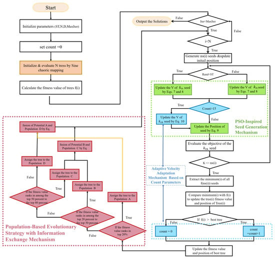
Figure 6.
The flowchart for the DTSA.
3.5. Time Complexity Analysis of DTSA
To study the time complexity of DTSA, it is crucial to understand the main components of the code and their frequencies of execution. The DTSA primarily comprises initialization, iterative updates, crossover operations, and natural selection. Here, is an analysis of the time complexities involved in each part.
Initialization: This stage employs Chebyshev chaotic mapping to generate random numbers for each dimension of every tree. With two nested loops—outer iterating N times (number of trees) and inner D times (problem dimensions)—the time complexity is estimated at .
Iterative update phase: Within a loop iterating up to a maximum of times, several key steps unfold. First, adaptive weight calculation occurs, which is computationally light with a time complexity of . Proceeding to seed generation, each tree produces a variable number of seeds within a dynamic range defined by ‘low’ and ‘high’, resulting in a complexity of . Estimating , the average number of seeds per tree as , calculating the fitness for each seed incurs a cost of . Updates to tree positions and tracking the best solution both occur with a linear time complexity, , while updating a counter is negligible at . Consequently, the aggregate time complexity for this iterative process is approximately .
Crossover and natural selection: This phase initiates with sorting trees based on fitness, demanding time. Segregation of the population follows swiftly with complexity. Crossover operations and natural selection, both executed in time, precede an analogous double-loop operation updating tree velocities and positions, also in . This segment, integrating sorting, population manipulation, genetic mechanisms, and status refreshes, accumulates to a total time complexity around .
In summary, while DTSA’s time complexity mirrors TSA’s in most procedural aspects, the crossover and natural selection phases introduce additional computational demands without fundamentally elevating the overall time complexity of the algorithm.
| Algorithm 1 The pseudo-code of the DTSA |
|
4. Results and Discussion
In this section, we present a series of experiments to assess the performance of the proposed DTSA. We analyze the advantages of DTSA based on six comprehensive experimental results. Additionally, Section 4.1 outlines the parameter configurations utilized in the upcoming experiments. The subsequent experiments’ parameter settings are introduced in detail, providing a comprehensive overview of the experimental setup. Subsequently, in Section 4.2, we initiate the exploration with the qualitative analysis of DTSA. Subsequently, in Section 4.3, we delve into the quantitative aspects of the analysis. Section 4.4 conducts an in-depth examination of the experimental data from the preceding quantitative analysis. Further reinforcing the significance of DTSA, Section 4.5 presents statistical experiments, demonstrating its superior performance compared to other algorithms. In Section 4.6, we extend the validation of DTSA by applying it to address three real-world problems.
4.1. Experiment Setting
DTSA underwent a comprehensive performance assessment by being pitted against various cutting-edge algorithms and several modifications. Notable contenders included EST-TSA [50], fb-TSA [51], TSA [34], STSA [42], MTSA [38], GA [58], PSO [57], GWO [59], BA [60], BOA, and RSA [61].
To ensure experimental fairness, this paper meticulously records the datasets and parameters employed by the comparison algorithms in the original research, as presented in Table 1. The experimental dataset is based on the IEEE CEC 2014 benchmark function, as indicated by the statistical results, where – are unimodal functions, – are simple multimodal functions, – are mixed functions, and – are combined functions [62]. Further details regarding the CEC 2014 benchmark function can be found in Table 2 and Table 3.

Table 1.
The initial parameters of comparative algorithms.

Table 2.
Definitions of the basic IEEE benchmark functions.

Table 3.
Benchmark functions of IEEE CEC 2014.
4.2. Qualitative Analysis
In order to qualitatively analyze the proposed algorithm, we conducted convergence behavior analysis, population diversity analysis, and exploration and exploitation analysis experiments to observe its performance. At the same time, we selected classical unimodal function to evaluate the development ability of the algorithm, and classical multimodal function to evaluate the exploration ability of the algorithm, as shown in Figure 7 and Figure 8.
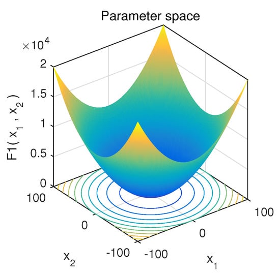
Figure 7.
Unimodal function F1.
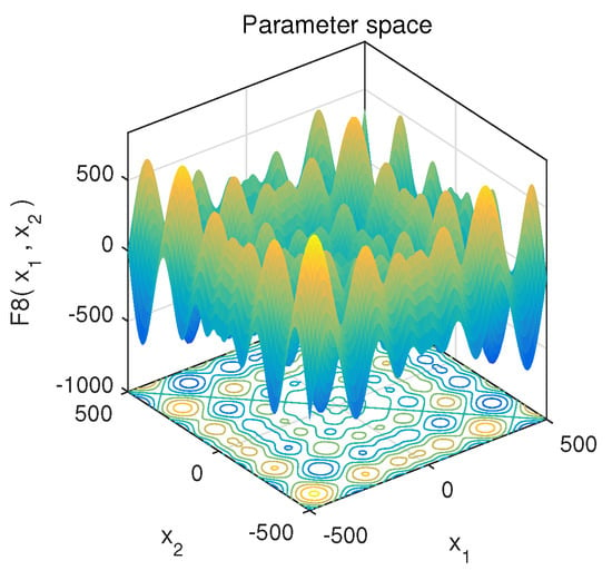
Figure 8.
Multimodal function F8.
4.2.1. Convergence Behavior Analysis
In this experiment, there are a total of four convergence analysis graphs ( in Figure 9 and Figure 10), the specific meanings of the four pictures of the different functions are as follows:
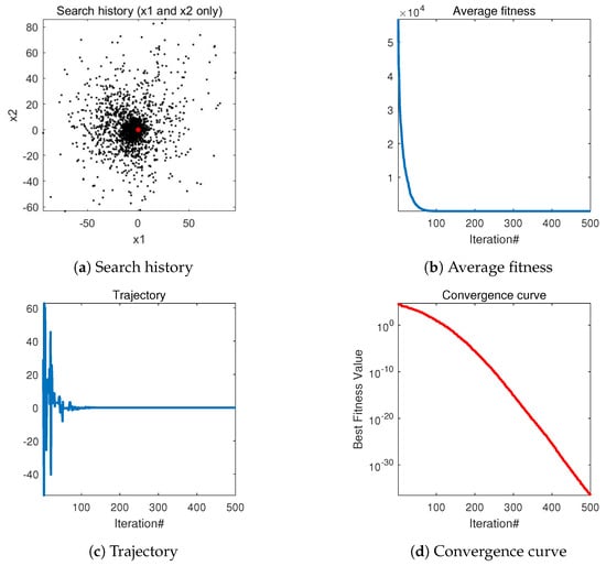
Figure 9.
The qualitative analysis of DTSA in unimodal function (F1) (search history (a), average fitness history (b), trajectory history (c), convergence curve (d)).
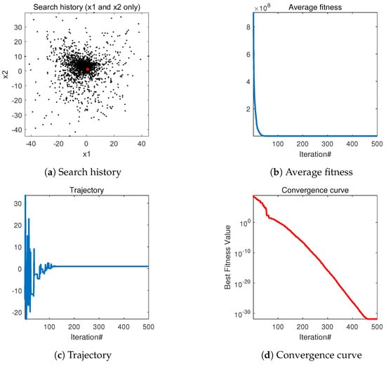
Figure 10.
The qualitative analysis of DTSA in multimodal function (F8) (search history (a), average fitness history (b), trajectory history (c), convergence curve (d)).
- The first image illustrates the optimization process of the DTSA algorithm. The black dots represent the areas covered by current seeds, while the red dot indicates the best position found, representing the optimal solution. The clustering of black dots around the red dot demonstrates the step-by-step optimization of DTSA towards convergence.
- The second figure depicts the convergence of DTSA, showcasing its rapid convergence towards the optimal solution. The sharp decline in the convergence curve underscores DTSA’s efficiency in finding optimal solutions.
- The third graph monitors changes in the first dimension, offering insights into the algorithm’s behavior and its avoidance of premature convergence to local optima. Empirical evidence suggests that the DTSA algorithm effectively navigates away from local optima.
- In the fourth graph, the convergence of the mean over multiple iterations is presented. The noticeable decline in the curve indicates the significant overall convergence effect of DTSA, further affirming its efficacy in optimization tasks.
4.2.2. Population Diversity Analysis
In optimization algorithms, population diversity serves as a pivotal metric for gauging efficiency. Its level has a direct impact on the exploration depth within the algorithm’s search space. A heightened population diversity is instrumental in averting entrapment in local optima, preserving the algorithm’s prowess for global search. This fosters a more extensive exploration of the search space during initial stages, thereby enhancing the likelihood of discovering the global optimal solution. This broadened search capability enables DTSA to adeptly handle problems with varying shapes and structures, mitigating over-optimization for specific instances. Consequently, the maintenance of appropriate population diversity emerges as a critical factor for ensuring the robustness and global search performance of algorithms. In practical applications, the mathematical formula for measuring population diversity can be used in various ways. In this paper, the dispersion of individual and collective centroids is used to represent population diversity, where Equations (17) and (18) are used to calculate the population diversity .
We easily observe from Figure 11 and Figure 12 that in the single-modal function , both DTSA and TSA exhibit a rapid decrease in population diversity. The algorithms exhibit strong local exploitation capabilities, facilitating the rapid identification of global optimum solutions. Despite this, DTSA demonstrates faster convergence compared to TSA while preserving higher population diversity throughout the process. For the multimodal function, DTSA benefits from the sine chaotic map for population initialization, resulting in increased diversity early in the algorithm and maintaining it through mid-term iterations. Although population diversity diminishes after encountering local optima, the count-based adaptive velocity update strategy enables DTSA to bolster diversity, aiding its escape from such solutions.
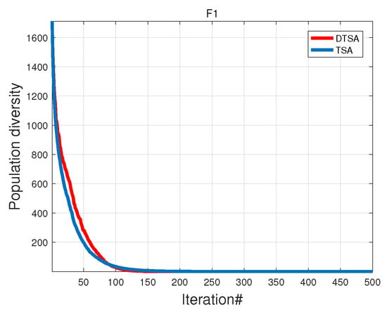
Figure 11.
Unimodal functions.
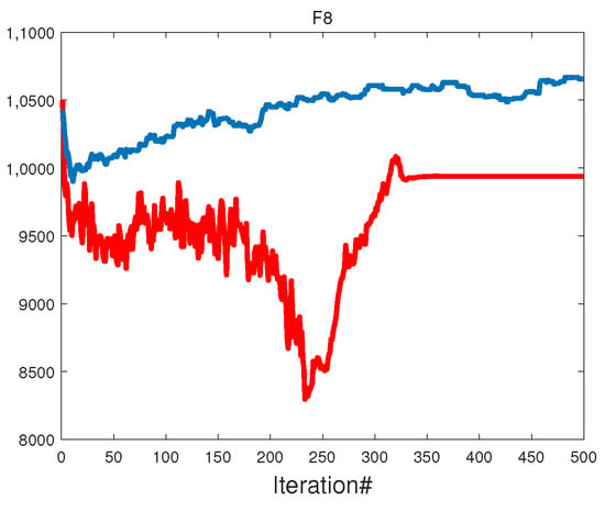
Figure 12.
Multimodal functions.
4.2.3. Exploration and Exploitation Analysis
In swarm intelligence optimization algorithms, exploring development analysis is often used to evaluate the exploration capability of the algorithm. The diversity of the swarm across iterations is a key factor in understanding how well the algorithm explores the solution space. The diversity at iteration t () can be calculated using the average distance between particles in the swarm by Equation (19):
This measures the average Euclidean distance between all pairs of particles in the swarm. The exploring development and the exploitation analysis can be defined as the ratio of the diversity at each iteration to the maximum diversity, as shown by Equations (20) and (21):
In Figure 13 and Figure 14, a higher value of indicates better exploration capacity and a higher value of indicates better exploitation capacity at iteration t. In comparing DTSA with the original algorithm, both demonstrate rapid development in single-mode function , indicating strong development capabilities. For multimode function , DTSA achieves a balance between development and exploration at 212 iterations, gradually decreasing exploration while maintaining excellent global exploration ability. In contrast, TSA reaches a balance at 1042 iterations, indicating good global exploration but with weaker practical applicability due to a maximum iteration limit of 500 iterations.
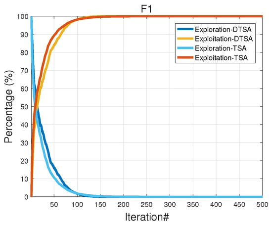
Figure 13.
Unimodal functions.
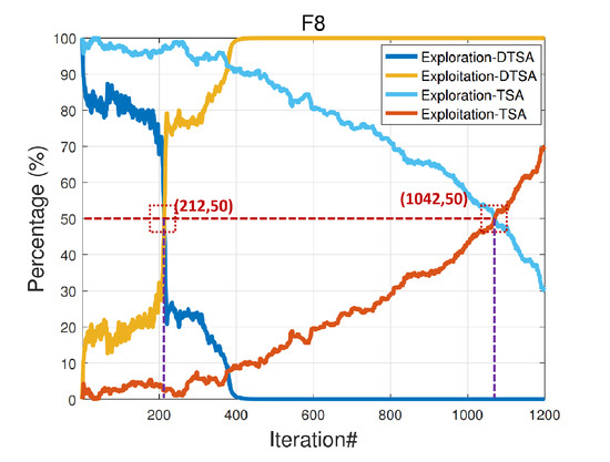
Figure 14.
Multimodal functions.
4.3. Quantitative Analysis
In this section, three strategically crafted experiments establish DTSA’s superior performance. Section 4.3.1 rigorously compares DTSA with various TSA variants, unequivocally demonstrating its superiority. Section 4.3.2 extends the comparison to include additional metaheuristic algorithms, highlighting DTSA’s exceptional ability to tackle intricate problems. Section 4.3.3 presents boxplots derived from 30 rounds of experiment results, offering visual insights into DTSA’s stability across multiple iterations.
4.3.1. Comparative Experiment 1: DTSA versus EST-TSA, fb-TSA, TSA, STSA, and MTSA
The first comparative experiment evaluates basic TSA [34] and its recent variants (EST-TSA [50], fb-TSA [51], STSA [42], and MTSA [38]) to showcase their strengths. Comparative assessments of DTSA and other algorithms across 30, 50, and 100 dimensions are presented in Table 4, Table 5 and Table 6. Additionally, graphical representations of the convergence curves for these algorithms are depicted in Figure 15, Figure 16 and Figure 17.

Table 4.
The mean values for the DTSA, EAT-TSA, fb-TSA, TSA, STSA, and MTSA in 30 dimensions.

Table 5.
The mean values for the DTSA, EAT-TSA, fb-TSA, TSA, STSA, and MTSA in 50 dimensions.

Table 6.
The mean values for the DTSA, EAT-TSA, fb-TSA, TSA, STSA, and MTSA in 100 dimensions.
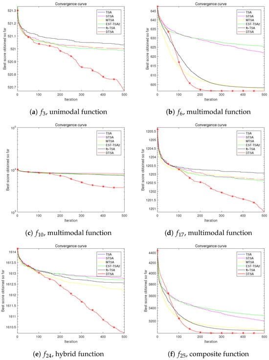
Figure 15.
Convergence curves of the DTSA and TSA and its recent variants in 30 dimensions.
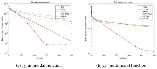
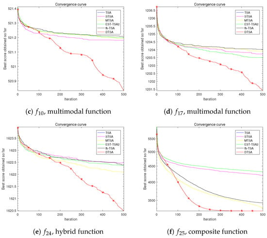
Figure 16.
Convergence curves of the DTSA and TSA and its recent variants in 50 dimensions.
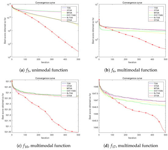
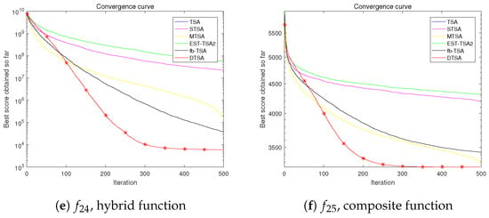
Figure 17.
Convergence curve of the DTSA and TSA and its recent variants in 100 dimensions.
The tables present the average optimal values obtained from 30 experimental iterations, each comprising 500 iterations, offering insights into the convergence performance of the algorithms. This aggregated data are crucial for discerning algorithmic superiority.
Moreover, meticulously documented convergence processes over 500 iterations for each experimental iteration shed light on performance dynamics. By averaging 30 local optimal solutions at each iteration point, the computed average convergence process reveals nuanced performance details. The slopes of these curves provide quantitative assessments of convergence speed.
The results underscore the efficacy of leveraging the fusion mechanism of tree population to enhance population diversity, thereby avoiding local optima. Additionally, refinements in the position update formula (Equation (9)) significantly improve convergence speed compared to previously proposed TSA variants.
Based on the empirical evidence, we confidently assert the superiority of the algorithm introduced in this study over other TSA algorithms and their variants in optimization endeavors.
4.3.2. Comparative Experiment 2: DTSA versus Classical and Recent Swarm Intelligence Algorithms
To substantiate the efficacy of the proposed algorithm, additional experiments were meticulously conducted. Classical swarm intelligence algorithms, including GA [58] and PSO [63], and some recent and famous swarm intelligence algorithms, such as RSA [64] and BOA [65], were deliberately chosen for comparative analyses.
The experimental setup rigorously adhered to the specifications outlined in Section 4.3.1, comprising 30 rounds of experiments with 500 iterations per round. Problem dimensions varied across 30, 50, and 100, maintaining consistency with earlier experiments. Furthermore, parameters for each algorithm were meticulously configured according to the settings outlined in their respective original papers, as delineated in Table 1.
Table 7, Table 8 and Table 9 document the average best values attained by DTSA and its counterparts across 30 rounds of experimentation, providing insights into the average rankings of each algorithm. These tables validate DTSA’s robust performance, particularly in addressing multimodal problems. Additionally, graphical depictions of convergence curves for these algorithms are illustrated in Figure 18, Figure 19 and Figure 20.

Table 7.
The mean values for the DTSA, EAT-TSA, fb_TSA, TSA, STSA, MTSA, PSO, GWO, BOA and RSA in 30 dimensions.

Table 8.
The mean values for the DTSA, EAT-TSA, fb_TSA, TSA, STSA, MTSA, PSO, GWO, BOA and RSA in 50 dimensions.

Table 9.
The mean values for the DTSA, EAT-TSA, fb_TSA, TSA, STSA, MTSA, PSO, GWO, BOA and RSA in 100 dimensions.
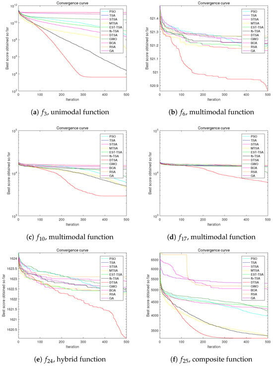
Figure 18.
Convergence curves of the DTSA and TSA and its recent variants in 30 dimensions.
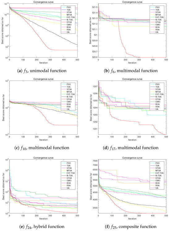
Figure 19.
Convergence curve of the DTSA and TSA and its recent variants in 50 dimensions.
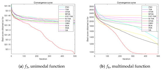
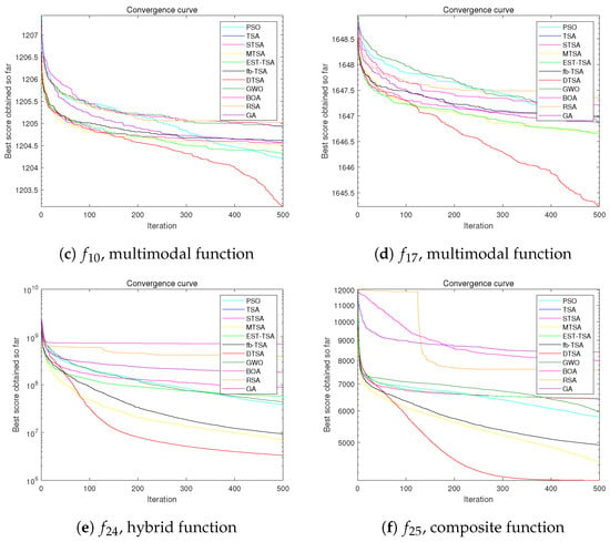
Figure 20.
Convergence curve of the DTSA and TSA and its recent variants in 100 dimensions.
4.3.3. Comparative Experiment 3: Analyzing the Stability of the DTSA
In this section, boxplots are presented to facilitate stability analysis of the DTSA algorithm. Figure 21, Figure 22 and Figure 23 depict these boxplots, with the x-axis representing the algorithm proposed in this study and other comparative algorithms. The y-axis shows objective function evaluations derived from 30 rounds of experiments for each algorithm.
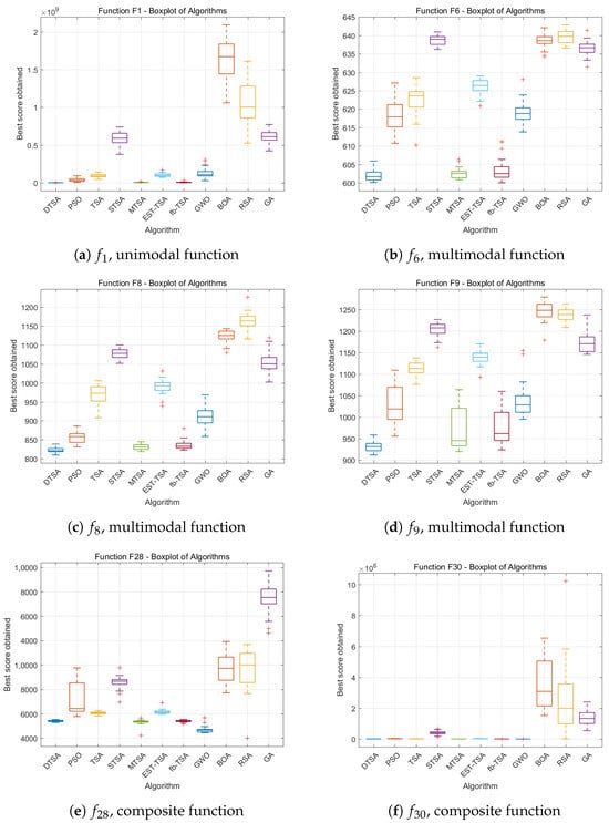
Figure 21.
Boxplots of all experiment algorithms in 30 dimensions.
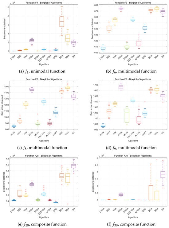
Figure 22.
Boxplots of all experiment algorithms in 50 dimensions.
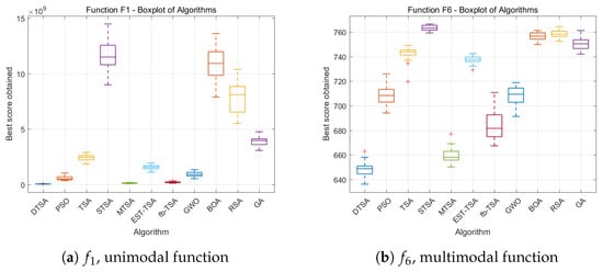
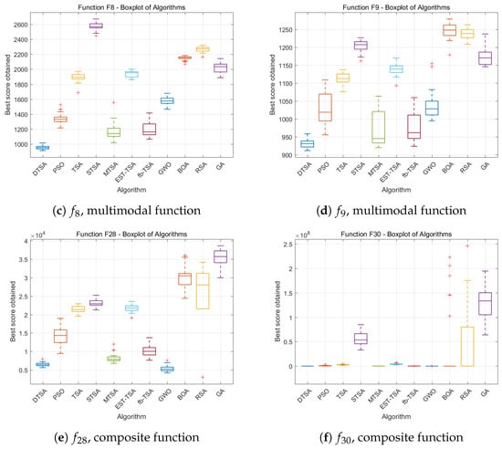
Figure 23.
Boxplots of all experiment algorithms in 100 dimensions.
Each plot displays uppermost and lowermost black lines representing maximum and minimum values from the 30 evaluations. The bounds of the box signify upper and lower quartiles, while the red line within the box indicates the median. Plus signs outside the box highlight outliers, denoting exceptional or subpar performance instances in specific rounds. This graphical representation aids in comprehensive assessment of the algorithm’s stability and performance across multiple experimental rounds.
Upon scrutinizing the comparative boxplots, it is evident that DTSA demonstrates commendable consistency in performance across various experimental setups. Its robust boxplot manifestations and minimal presence of outliers substantiate DTSA’s capability to consistently yield favorable results in diverse experimental environments, affirming its distinguished attribute of elevated stability. This empirical validation underscores DTSA’s reliability and effectiveness in optimization tasks, confirming its utility in complex problem-solving scenarios with confidence.
In summary, DTSA’s performance in the quantitative analysis highlights a substantial boost in its optimization efficacy. By integrating a PSO-inspired seed generation mechanism and a count-based adaptive strategy, it effectively addresses the traditional TSA’s limitations regarding premature convergence and challenges with high-dimensional, intricate optimization issues. Notably, the experiments not only validate DTSA’s superiority through comparisons with numerous cutting-edge algorithms but also reinforce its efficiency and stability in real-world problem applications. The comprehensive assessment on the IEEE CEC 2014 benchmark functions demonstrates DTSA’s rapid and steady convergence trend, particularly excelling in navigating multimodal, mixed, and composite functions by adeptly avoiding local optima to reach global optimality.
However, when confronted with simplistic, unimodal functions, where all algorithms effortlessly locate the optimal solution due to the inherently low complexity, the enhancements brought by DTSA become less conspicuous. In alignment with the no free lunch theorem [44], it is a recognized fact that no single algorithm can universally prevail in every scenario; their superiority is inherently tied to the specific complexities embedded within each distinct problem. Hence, it is inevitable that DTSA exhibits a differentiated effectiveness, finely attuned to the intricacy and dimensional breadth of the tasks it encounters.
4.4. Further Analysis
To elucidate the performance characteristics of DTSA, it is imperative to undertake an advanced analysis that integrates findings from both qualitative and quantitative investigations. This approach will provide a comprehensive understanding of the experimental observations associated with DTSA’s functionality.
Firstly, DTSA showcases superior performance over several TSA variants, as it integrates three key innovative mechanisms that collectively enhance its operational efficiency. These innovations significantly improve DTSA’s adaptability, diversity, and convergence speed. By dynamically updating seed positions, adjusting search behavior to prevent premature convergence, and incorporating genetic diversity through arithmetic crossover and natural selection, DTSA achieves a remarkable balance between exploration and exploitation. This strategic combination not only accelerates the algorithm’s convergence towards optimal solutions but also maintains a high level of population diversity, setting DTSA apart in optimization tasks and showcasing its advanced capability in handling complex optimization problems
Secondly, in addressing low-dimensional optimization challenges, DTSA does not exhibit a marked superiority over competing algorithms, attributable to its sophisticated mechanisms primarily optimized for the intricacies of high-dimensional search spaces. These mechanisms, while potent in navigating and exploiting the complex landscapes of high-dimensional problems, yield diminishing returns in less complex, low-dimensional scenarios. Consequently, the inherent advantage of DTSA’s advanced features becomes less pronounced, as simpler algorithmic solutions prove equally adept in these contexts. This observation underscores a critical avenue for future research aimed at refining DTSA’s adaptability and efficiency across a diverse array of problem scales, thereby enhancing its utility in a wider spectrum of optimization tasks.
Thirdly, the empirical evidence, as delineated by the boxplot visualizations in Figure 21, Figure 22 and Figure 23, unequivocally establishes the superior stability and quality of DTSA in comparison to the algorithms it was tested against within this study. Specifically, the more compact and lower interquartile ranges of DTSA’s boxplots for certain functions distinctly underscore its enhanced performance metrics. This excellence is directly attributable to the innovative integration of the tree population integrated evolutionary strategy and adaptive velocity-driven seed generation mechanisms, as introduced in this research. These methodologies empower the DTSA to dynamically refine the optimization trajectory across varied benchmark function evaluations, culminating in reduced variability (as evidenced by smaller standard deviations) and improved reliability in experimental outcomes. This adaptability and precision in handling diverse optimization scenarios underscore the algorithm’s robustness and its potential applicability in solving complex optimization problems with heightened efficiency and consistency.
4.5. Statistical Experiments
Table 10 presents the outcomes of the Wilcoxon’s signed-rank test applied to the experimental data of the DTSA algorithm in comparison to 11 other algorithms [66]. The table includes p-values obtained at the significance level . Columns labeled TRUE and FALSE indicate whether the hypothesis is rejected or not rejected at the specified significance level of . The data for this analysis are sourced from the comparative experiments detailed in Section 4.3, ensuring consistency with the experimental setup.

Table 10.
Results of Wilcoxon’s test for DTSA and other algorithms.
Our assertion is that DTSA demonstrates superior performance compared to the other algorithms. A smaller p-value resulting from the experiment between DTSA and a comparative algorithm, below the significance level , indicates DTSA’s superior performance. Table 10 reveals that DTSA consistently exhibits very low p-values compared to the majority of the algorithms. Consequently, under both significance levels ( = 0.1 and = 0.05), our hypothesis is confirmed. These findings affirm that, in this experiment, the DTSA algorithm significantly outperforms the other algorithms in terms of performance.
4.6. Practical Engineering Problems of Mathematical Modeling
In light of the advanced analysis delineated in Section 4.4, which evidences the Dynamic Tree-Seed Algorithm’s (DTSA) proficiency in navigating high-dimensional complex problem spaces, this section is dedicated to an empirical evaluation of DTSA’s adeptness in addressing complex constrained optimization challenges. Specifically, we scrutinize its performance through the lens of intricate objective functions and multifarious constraints, employing a suite of benchmark problems for this purpose: Tension spring design [67], three-bar truss design [68], welded beam design [69], cantilever beam design [70], and step-cone pulley design problems [71]. The analytical results, encapsulated in Table 11, Table 12, Table 13, Table 14 and Table 15, are articulated through several statistical measures: best signifies the optimal value achieved by DTSA across 30 experimental iterations; mean delineates the average result; std refers to the standard deviation, indicating result variability; worst captures the least favorable outcome; and the x denotes the optimal solution configuration ascertained by DTSA at the juncture of achieving its best result. This methodological approach affords a rigorous assessment of DTSA’s capability to effectively resolve complex constrained optimization tasks, furnishing a comprehensive perspective on its performance efficacy.
4.6.1. Example 1: Tension Spring Design Problem
The pressure vessel design (PVD) problem aims to minimize the total cost, denoted as , while satisfying the production requirements. This optimization problem is defined by four design variables: the shell thickness , the head thickness , the inner radius , and the length of the vessel , excluding the head. Both and are quantized in multiples of , whereas R and L are considered as continuous variables. The mathematical model of the pressure vessel design (PVD) problem is detailed from [67]:
Objective function:
Subject to constraints:
Variable bounds:
The results of the tension spring design problem are shown in Table 11. The results show that the DTSA has better performance.


Table 11.
Tension spring design problem.
Table 11.
Tension spring design problem.
| DTSA | TSA | DBO | HHO | GWO | SO | WFO | GOA | |
|---|---|---|---|---|---|---|---|---|
| Best | 0.013 | 0.013 | 0.013 | 0.014 | 0.013 | 0.013 | 0.018 | 0.013 |
| Mean | 0.013 | 0.013 | 0.013 | 0.015 | 0.013 | 0.013 | 0.036 | 0.014 |
| Std | 0.000 | 0.000 | 0.000 | 0.001 | 0.000 | 0.000 | 0.026 | 0.001 |
| Worst | 0.000 | 0.013 | 0.013 | 0.016 | 0.013 | 0.013 | 0.054 | 0.015 |
| 0.053 | 0.053 | 0.050 | 0.060 | 0.050 | 0.050 | 0.068 | 0.058 | |
| 0.389 | 0.381 | 0.317 | 0.597 | 0.319 | 0.317 | 0.872 | 0.521 | |
| 9.602 | 10.015 | 14.028 | 4.426 | 13.918 | 14.028 | 2.439 | 5.648 |
4.6.2. Example 2: Three-Bar Truss Design Problem
The efficacy of the algorithm is evaluated in test 2, utilizing the three-bar truss design problem. The primary objective is to minimize the volumetric attribute of the statically loaded three-bar truss, constrained by a triplet of inequality conditions. The optimization’s objective function is structured to compute the optimal cross-sectional areas corresponding to the design variables, denoted as and . This delineation is emblematic of structural optimization paradigms, where the optimization of material usage and adherence to mechanical constraints are of critical importance, thus providing a stringent assessment of the algorithm’s navigational acumen within multifaceted design domains.
Consider ,
Objective function:
Subject to constraints:
Where:
Variable bounds:
The results of the three-bar truss design problem are shown in Table 12. The results show that the DTSA has better performance.


Table 12.
Three-bar truss design problem.
Table 12.
Three-bar truss design problem.
| DTSA | TSA | DBO | HHO | GWO | SO | WFO | GOA | |
|---|---|---|---|---|---|---|---|---|
| Best | 263.8958 | 2.64 × | 263.8963 | 263.9051 | 263.8982 | 263.8959 | 265.4799 | 263.9054 |
| Mean | 263.8958 | 263.8958 | 263.8968 | 264.0205 | 263.9012 | 263.8969 | 265.5999 | 263.975 |
| Std | 2.81 × | 3.91 × | 7.95 × | 0.163226 | 4.28 × | 0.001494 | 0.169762 | 0.098407 |
| Worst | 2.64 × | 263.8959 | 263.8974 | 264.1359 | 263.9043 | 263.898 | 265.4799 | 264.0446 |
| 0.7886 | 0.7887 | 0.7879 | 0.7851 | 0.7895 | 0.7885 | 0.822665 | 0.785091 | |
| 0.4082 | 0.4081 | 0.4104 | 0.4182 | 0.4059 | 0.4087 | 0.3279 | 0.4184 |
4.6.3. Example 3: Welded Beam Design Problem
The welded beam design (WBD) problem is a classical optimization task that seeks to minimize the manufacturing cost of a beam’s design. The problem is defined by four design variables: the beam’s length l, height t, thickness b, and the weld thickness h. The objective of the optimization process is to ascertain the values of these variables that result in the minimum production cost while adhering to the constraints imposed by shear stress , bending stress , buckling load on the bar , end deflection , and other prescribed boundary conditions. The WBD problem thus serves as a paradigmatic nonlinear programming challenge, wherein the cost function is intricately linked with a set of physical constraints that are interdependent. The mathematical formulation of the WBD problem is as follows:
Variables:
Objective function:
Variable bounds:
Subject to constraints:
where:

Table 13.
Welded beam design problem.
Table 13.
Welded beam design problem.
| DTSA | TSA | DBO | HHO | GWO | SO | WFO | GOA | |
|---|---|---|---|---|---|---|---|---|
| Best | 1.6927 | 1.6927 | 1.6927 | 1.7399 | 1.6954 | 1.6928 | 1.9850 | 2.3256 |
| Mean | 1.6927 | 1.6927 | 1.6927 | 1.7838 | 1.6957 | 1.6940 | 2.0007 | 2.6348 |
| Std | 0 | 1.03 × | 5.55 × | 0.0620 | 0.0004 | 0.001 | 0.02226 | 0.4372 |
| Worst | 1.6927 | 1.6927 | 1.6927 | 1.8276 | 1.6960 | 1.6951 | 2.0164 | 2.9439 |
| 0.2057 | 0.2057 | 0.2057 | 0.1877 | 0.2055 | 0.2057 | 0.24336 | 0.278417 | |
| 3.2349 | 3.2349 | 3.2349 | 3.5996 | 3.2416 | 3.2346 | 2.8060 | 3.1226 | |
| 9.0366 | 9.0366 | 9.0366 | 9.2250 | 9.0506 | 9.0372 | 8.5761 | 6.7455 | |
| 0.2057 | 0.2057 | 0.2057 | 0.2048 | 0.2056 | 0.2057 | 0.2597 | 0.3704 |
4.6.4. Example 4: Cantilever Beam Design Problem
The cantilever beam optimization problem represents a fundamental structural engineering design challenge focused on the weight reduction of a cantilever beam featuring a square cross-section. This beam is characterized by a fixed support at one end and experiences a vertical load at the free end. Comprised of five hollow square segments of uniform thickness—specifically, 2/3 of an inch—the primary design variables are the heights or widths of these segments. The optimization seeks to minimize the total weight while ensuring compliance with structural requirements, including stress limits, deflection tolerances, and vibrational characteristics. It also considers practical aspects such as manufacturability and cost-effectiveness. The mathematical model encapsulating this optimization problem involves an objective function for weight calculation and a set of constraints ensuring the beam’s structural feasibility and functional adequacy under applied loads. This problem can be represented by the following mathematical equation:
Objective function:
Subject to constraints:
Variable bounds:
The results of the cantilever beam design problem are shown in Table 14. The results show that the DTSA has better performance.


Table 14.
Cantilever beam design problem.
Table 14.
Cantilever beam design problem.
| DTSA | TSA | DBO | HHO | GWO | SO | WFO | GOA | |
|---|---|---|---|---|---|---|---|---|
| Best | 1.3399 | 1.3399 | 1.3399 | 1.3437 | 1.3400 | 1.3400 | 2.6214 | 1.3737 |
| Mean | 1.3399 | 1.3399 | 1.3399 | 1.3440 | 1.3400 | 1.3400 | 2.6740 | 1.4063 |
| Std | 2.08 × | 7.40 × | 6.63 × | 0.0004 | 5.03 × | 2.11 × | 0.0743 | 0.0462 |
| Worst | 1.3399 | 1.3399 | 1.3399 | 1.3443 | 1.3401 | 1.3400 | 2.7266 | 1.4390 |
| 6.0161 | 6.0192 | 6.0354 | 5.8279 | 6.0266 | 5.9732 | 4.9741 | 5.9102 | |
| 5.3094 | 5.3085 | 5.3191 | 5.2299 | 5.2760 | 5.3042 | 16.3215 | 6.0045 | |
| 4.4947 | 4.4934 | 4.4922 | 4.8202 | 4.4834 | 4.5395 | 7.1959 | 3.9133 | |
| 3.5007 | 3.4994 | 3.4801 | 3.4528 | 3.5322 | 3.5006 | 10.6454 | 4.1481 | |
| 2.1525 | 2.1529 | 2.1471 | 2.2033 | 2.1565 | 2.1575 | 2.8738 | 2.0382 |
4.6.5. Example 5: Step-Cone Pulley Problem
The step-cone pulley design problem is a weight minimization task encountered in structural engineering, focusing on the optimization of a multi-stepped pulley system. Each step of the pulley, with a distinct diameter, contributes to the overall design that must adhere to specific mechanical constraints and performance goals. The challenge lies in determining the optimal configuration of these diameters and other design aspects to achieve minimal weight without compromising the pulley’s functional integrity. This problem is emblematic of complex engineering design tasks, which require sophisticated optimization techniques to solve due to their nonlinear and constrained nature.
Objective function:
Subject to constraints:
Where:
The results of the step-cone pulley problem are shown in Table 15. The results show that the DTSA has better performance.


Table 15.
Step-cone pulley problem.
Table 15.
Step-cone pulley problem.
| DTSA | TSA | DBO | HHO | GWO | SO | WFO | GOA | |
|---|---|---|---|---|---|---|---|---|
| Best | 1.67 × | 2.84 × | 1.67 × | 4.60 × | 4.31 × | 1.67 × | 6.77 × | 4.86 × |
| Mean | 1.67 × | 2.49 × | 1.75 × | 2.17 × | 8.53 × | 1.44 × | 1.03 × | 3.01 × |
| Std | 1.17 × | 3.51 × | 1.08 × | 3.07 × | 5.97 × | 2.03 × | 5.00 × | 4.25 × |
| Worst | 1.68 × | 4.97 × | 1.83 × | 4.34 × | 1.28 × | 2.87 × | 1.38 × | 6.01 × |
| 3.98 × | 3.91 × | 4.00 × | 3.97 × | 3.95 × | 3.89 × | 5.82 × | 3.89 × | |
| 5.47 × | 5.38 × | 5.50 × | 5.46 × | 5.44 × | 5.35 × | 5.98 × | 5.35 × | |
| 7.29 × | 7.17 × | 7.33 × | 7.28 × | 7.26 × | 7.14 × | 7.78 × | 7.14 × | |
| 8.75 × | 8.59 × | 8.79 × | 8.73 × | 8.70 × | 8.56 × | 8.23 × | 8.55 × | |
| 8.69 × | 8.92 × | 8.65 × | 8.73 × | 8.95 × | 8.99 × | 8.81 × | 8.92 × |
5. Conclusions and Future Work
The Dynamic Tree-Seed Algorithm presents a series of quantitative improvements over existing optimization algorithms, which can be specifically highlighted in terms of numerical results and comparative evaluations. In the studies and experiments conducted, DTSA demonstrates its efficacy through the following achievements:
- Performance enhancement: DTSA was tested against various benchmarks and recent TSA variants such as STSA, EST-TSA, fb-TSA, and MTSA, along with established algorithms like GA, PSO, GWO, BA, and RSA. It consistently outperformed these algorithms across multiple dimensions (30D, 50D, 100D) and on different types of functions (unimodal, multimodal, composite), as shown in the IEEE CEC 2014 benchmark tests.
- Convergence and robustness: The convergence curves depicted in figures like Figure 17 illustrate DTSA’s faster convergence rate and stability even in higher dimensional spaces and for complex functions such as hybrid and composite ones. This indicates that DTSA effectively balances exploration and exploitation, leading to quicker and more accurate solutions.
- Statistical measures: Across experiments, DTSA’s performance was quantified using measures like best, mean, std (standard deviation), worst, and X (optimal solution configuration). These metrics provided a comprehensive view of its effectiveness, showing consistent superiority in finding optimal or near-optimal solutions with reduced variability.
- Engineering applications: When applied to real-world engineering problems like tension spring design, three-bar truss design, and others, DTSA achieved optimal values, as documented in Table 11, Table 12, Table 13, Table 14 and Table 15, indicating its practical utility and robustness in solving constrained optimization tasks.
These outcomes and comparisons solidify DTSA’s scientific contribution by offering a quantifiable advancement in optimization efficiency, accuracy, and versatility across a broad spectrum of problem domains.
6. Research Constraints and Considerations
While DTSA has undeniably demonstrated significant enhancements in its optimization capabilities, particularly excelling in addressing high-dimensional and multimodal optimization problems, there remain several aspects warranting further exploration and refinement to augment its versatility and practical utility. These areas include:
Firstly, the algorithm’s universality and generalization capacity: Despite impressive performances on numerous IEEE CEC 2014 benchmark functions, DTSA’s advancements are less pronounced in scenarios involving simple structures or unimodal functions. This suggests a need for refining the algorithm to better accommodate diverse problem characteristics, encompassing low-dimensional and straightforward optimization scenarios, thus elevating its generalization prowess.
Secondly, parameter tuning and sensitivity: DTSA’s performance is significantly influenced by meticulous parameter calibration. Presently, research on parameter selection and tuning strategies might not delve deep enough, necessitating a more systematic analysis of parameter sensitivity. This would facilitate the establishment of default or adaptive parameter settings applicable to a broader spectrum of problems, alleviating the user’s burden in manual parameter adjustments.
Lastly, computational efficiency for large-scale problems: As problem dimensions escalate, so do DTSA’s computational costs and memory requirements, potentially impeding its application to ultra-large-scale optimization tasks. Advancements in search strategies and data structures, or the incorporation of distributed computing frameworks to parallelize the algorithm, emerge as promising avenues to enhance the efficiency of tackling such massive problems.
To facilitate further research and practical application, we have made the source code publicly accessible at www.jianhuajiang.com (accessed on 1 June 2024), enabling the community to engage with and enhance the algorithm.
Author Contributions
J.J. and J.H. conceived and designed the methodology and experiments; J.H. performed the experiments, analyzed the results and wrote the paper; J.H., J.W., J.L., X.Y. and W.L. revised the paper. All authors have read and agreed to the published version of the manuscript.
Funding
The authors thank the financial support from the Foundation of the Jilin Provincial Department of Science and Technology (No. YDZJ202201ZYTS565), the Foundation of Social Science of Jilin Province, China (No. 2022B84) and the Jilin Provincial Department of Education Science and Technology (No. JJKH20240198KJ).
Data Availability Statement
Data are contained within the article.
Conflicts of Interest
The authors declare no conflict of interest.
References
- Kirkpatrick, S.; Gelatt, C.D.; Vecchi, M.P. Optimization by Simulated Annealing. Science 1983, 220, 671–680. [Google Scholar] [CrossRef] [PubMed]
- Homaifar, A.; Qi, C.X.; Lai, S.H. Constrained optimization via genetic algorithms. Simulation 1994, 62, 242–253. [Google Scholar] [CrossRef]
- Deb, K. An efficient constraint handling method for genetic algorithms. Comput. Methods Appl. Mech. Eng. 2000, 186, 311–338. [Google Scholar] [CrossRef]
- Liao, T.W. Two hybrid differential evolution algorithms for engineering design optimization. Appl. Soft Comput. 2010, 10, 1188–1199. [Google Scholar] [CrossRef]
- Yildiz, K.; Lesieutre, G.A. Sizing and prestress optimization of Class-2 tensegrity structures for space boom applications. Eng. Comput. 2022, 38, 1451–1464. [Google Scholar] [CrossRef]
- Osaba, E.; Villar-Rodriguez, E.; Del Ser, J.; Nebro, A.J.; Molina, D.; Latorre, A.; Suganthan, P.N.; Coello, C.A.C.; Herrera, L.E.F. A Tutorial On the design, experimentation and application of metaheuristic algorithms to real-World optimization problems. Swarm Evol. Comput. 2021, 64, 100888. [Google Scholar] [CrossRef]
- Tang, J.; Liu, G.; Pan, Q. A review on representative swarm intelligence algorithms for solving optimization problems: Applications and trends. IEEE/CAA J. Autom. Sin. 2021, 8, 1627–1643. [Google Scholar] [CrossRef]
- Tian, Y.; Si, L.; Zhang, X.; Cheng, R.; He, C.; Tan, K.C.; Jin, Y. Evolutionary large-scale multi-objective optimization: A survey. ACM Comput. Surv. (CSUR) 2021, 54, 1–34. [Google Scholar] [CrossRef]
- Lodi, A.; Martello, S.; Vigo, D. Heuristic and metaheuristic approaches for a class of two-dimensional bin packing problems. INFORMS J. Comput. 1999, 11, 345–357. [Google Scholar] [CrossRef]
- Li, S.; Chen, H.; Wang, M.; Heidari, A.A.; Mirjalili, S. Slime mould algorithm: A new method for stochastic optimization. Future Gener. Comput. Syst. 2020, 111, 300–323. [Google Scholar] [CrossRef]
- Hussain, K.; Mohd Salleh, M.N.; Cheng, S.; Shi, Y. Metaheuristic research: A comprehensive survey. Artif. Intell. Rev. 2019, 52, 2191–2233. [Google Scholar] [CrossRef]
- Gharehchopogh, F.S. Quantum-inspired metaheuristic algorithms: Comprehensive survey and classification. Artif. Intell. Rev. 2023, 56, 5479–5543. [Google Scholar] [CrossRef]
- Braik, M.; Sheta, A.; Al-Hiary, H. A novel meta-heuristic search algorithm for solving optimization problems: Capuchin search algorithm. Neural Comput. Appl. 2021, 33, 2515–2547. [Google Scholar] [CrossRef]
- Jiang, J.; Wu, J.; Luo, J.; Yang, X.; Huang, Z. MOBCA: Multi-Objective Besiege and Conquer Algorithm. Biomimetics 2024, 9, 316. [Google Scholar] [CrossRef] [PubMed]
- Parejo, J.A.; Ruiz-Cortés, A.; Lozano, S.; Fernandez, P. Metaheuristic optimization frameworks: A survey and benchmarking. Soft Comput. 2012, 16, 527–561. [Google Scholar] [CrossRef]
- Abualigah, L. Group search optimizer: A nature-inspired meta-heuristic optimization algorithm with its results, variants, and applications. Neural Comput. Appl. 2021, 33, 2949–2972. [Google Scholar] [CrossRef]
- Bai, J.; Jia, L.; Peng, Z. A new insight on augmented Lagrangian method with applications in machine learning. J. Sci. Comput. 2024, 99, 53. [Google Scholar] [CrossRef]
- Lin, Y.; Bian, Z.; Liu, X. Developing a dynamic neighborhood structure for an adaptive hybrid simulated annealing–tabu search algorithm to solve the symmetrical traveling salesman problem. Appl. Soft Comput. 2016, 49, 937–952. [Google Scholar] [CrossRef]
- Xue, X.; Chen, J. Using compact evolutionary tabu search algorithm for matching sensor ontologies. Swarm Evol. Comput. 2019, 48, 25–30. [Google Scholar] [CrossRef]
- Li, J.; Pardalos, P.M.; Sun, H.; Pei, J.; Zhang, Y. Iterated local search embedded adaptive neighborhood selection approach for the multi-depot vehicle routing problem with simultaneous deliveries and pickups. Expert Syst. Appl. 2015, 42, 3551–3561. [Google Scholar] [CrossRef]
- Derbel, H.; Jarboui, B.; Hanafi, S.; Chabchoub, H. Genetic algorithm with iterated local search for solving a location-routing problem. Expert Syst. Appl. 2012, 39, 2865–2871. [Google Scholar] [CrossRef]
- Vrugt, J.A.; Robinson, B.A.; Hyman, J.M. Self-adaptive multimethod search for global optimization in real-parameter spaces. IEEE Trans. Evol. Comput. 2008, 13, 243–259. [Google Scholar] [CrossRef]
- Deng, W.; Xu, J.; Song, Y.; Zhao, H. Differential evolution algorithm with wavelet basis function and optimal mutation strategy for complex optimization problem. Appl. Soft Comput. 2021, 100, 106724. [Google Scholar] [CrossRef]
- Das, S.; Abraham, A.; Chakraborty, U.K.; Konar, A. Differential evolution using a neighborhood-based mutation operator. IEEE Trans. Evol. Comput. 2009, 13, 526–553. [Google Scholar] [CrossRef]
- Wang, D.; Tan, D.; Liu, L. Particle swarm optimization algorithm: An overview. Soft Comput. 2018, 22, 387–408. [Google Scholar] [CrossRef]
- Zhang, Y.; Wang, S.; Ji, G. A comprehensive survey on particle swarm optimization algorithm and its applications. Math. Probl. Eng. 2015, 2015, 931256. [Google Scholar] [CrossRef]
- Kıran, M.S.; Fındık, O. A directed artificial bee colony algorithm. Appl. Soft Comput. 2015, 26, 454–462. [Google Scholar] [CrossRef]
- Xue, Y.; Jiang, J.; Zhao, B.; Ma, T. A self-adaptive artificial bee colony algorithm based on global best for global optimization. Soft Comput. 2018, 22, 2935–2952. [Google Scholar] [CrossRef]
- Gandomi, A.H.; Alavi, A.H. Krill herd: A new bio-inspired optimization algorithm. Commun. Nonlinear Sci. Numer. Simul. 2012, 17, 4831–4845. [Google Scholar] [CrossRef]
- Bolaji, A.L.; Al-Betar, M.A.; Awadallah, M.A.; Khader, A.T.; Abualigah, L.M. A comprehensive review: Krill Herd algorithm (KH) and its applications. Appl. Soft Comput. 2016, 49, 437–446. [Google Scholar] [CrossRef]
- Rashedi, E.; Rashedi, E.; Nezamabadi-Pour, H. A comprehensive survey on gravitational search algorithm. Swarm Evol. Comput. 2018, 41, 141–158. [Google Scholar] [CrossRef]
- Taradeh, M.; Mafarja, M.; Heidari, A.A.; Faris, H.; Aljarah, I.; Mirjalili, S.; Fujita, H. An evolutionary gravitational search-based feature selection. Inf. Sci. 2019, 497, 219–239. [Google Scholar] [CrossRef]
- MiarNaeimi, F.; Azizyan, G.; Rashki, M. Horse herd optimization algorithm: A nature-inspired algorithm for high-dimensional optimization problems. Knowl.-Based Syst. 2021, 213, 106711. [Google Scholar] [CrossRef]
- Kiran, M.S. TSA: Tree-seed algorithm for continuous optimization. Expert Syst. Appl. 2015, 42, 6686–6698. [Google Scholar] [CrossRef]
- El-Fergany, A.A.; Hasanien, H.M. Tree-seed algorithm for solving optimal power flow problem in large-scale power systems incorporating validations and comparisons. Appl. Soft Comput. 2018, 64, 307–316. [Google Scholar] [CrossRef]
- Jiang, J.; Yang, X.; Li, M.; Chen, T. ATSA: An Adaptive Tree Seed Algorithm based on double-layer framework with tree migration and seed intelligent generation. Knowl.-Based Syst. 2023, 279, 110940. [Google Scholar] [CrossRef]
- Jiang, J.; Wu, J.; Meng, X.; Qian, L.; Luo, J.; Li, K. Katsa: Knn Ameliorated Tree-Seed Algorithm for Complex Optimization Problems. Available online: https://papers.ssrn.com/sol3/papers.cfm?abstract_id=4636664 (accessed on 1 June 2024).
- Jiang, J.; Meng, X.; Qian, L.; Wang, H. Enhance tree-seed algorithm using hierarchy mechanism for constrained optimization problems. Expert Syst. Appl. 2022, 209, 118311. [Google Scholar] [CrossRef]
- Beşkirli, M. Solving continuous optimization problems using the tree seed algorithm developed with the roulette wheel strategy. Expert Syst. Appl. 2021, 170, 114579. [Google Scholar] [CrossRef]
- Beşkirli, A.; Özdemir, D.; Temurtaş, H. A comparison of modified tree–seed algorithm for high-dimensional numerical functions. Neural Comput. Appl. 2020, 32, 6877–6911. [Google Scholar] [CrossRef]
- Caponetto, R.; Fortuna, L.; Fazzino, S.; Xibilia, M.G. Chaotic sequences to improve the performance of evolutionary algorithms. IEEE Trans. Evol. Comput. 2003, 7, 289–304. [Google Scholar] [CrossRef]
- Jiang, J.; Xu, M.; Meng, X.; Li, K. STSA: A sine Tree-Seed Algorithm for complex continuous optimization problems. Phys. A Stat. Mech. Appl. 2020, 537, 122802. [Google Scholar] [CrossRef]
- Bajer, D.; Martinović, G.; Brest, J. A population initialization method for evolutionary algorithms based on clustering and Cauchy deviates. Expert Syst. Appl. 2016, 60, 294–310. [Google Scholar] [CrossRef]
- Wolpert, D.H.; Macready, W.G. No free lunch theorems for optimization. IEEE Trans. Evol. Comput. 1997, 1, 67–82. [Google Scholar] [CrossRef]
- Zheng, Y.; Li, L.; Qian, L.; Cheng, B.; Hou, W.; Zhuang, Y. Sine-SSA-BP ship trajectory prediction based on chaotic mapping improved sparrow search algorithm. Sensors 2023, 23, 704. [Google Scholar] [CrossRef] [PubMed]
- Beşkirli, M.; Kiran, M.S. Optimization of Butterworth and Bessel Filter Parameters with Improved Tree-Seed Algorithm. Biomimetics 2023, 8, 540. [Google Scholar] [CrossRef]
- Jiang, J.; Liu, Y.; Zhao, Z. TriTSA: Triple Tree-Seed Algorithm for dimensional continuous optimization and constrained engineering problems. Eng. Appl. Artif. Intell. 2021, 104, 104303. [Google Scholar] [CrossRef]
- Jiang, J.; Han, R.; Meng, X.; Li, K. TSASC: Tree–seed algorithm with sine–cosine enhancement for continuous optimization problems. Soft Comput. 2020, 24, 18627–18646. [Google Scholar] [CrossRef]
- Linden, A. ITSA: Stata Module to Perform Interrupted Time Series Analysis for Single and Multiple Groups. 2021. Available online: https://ideas.repec.org/c/boc/bocode/s457793.html (accessed on 1 June 2024).
- Jiang, J.; Jiang, S.; Meng, X.; Qiu, C. EST-TSA: An effective search tendency based to tree seed algorithm. Phys. A Stat. Mech. Appl. 2019, 534, 122323. [Google Scholar] [CrossRef]
- Jiang, J.; Meng, X.; Chen, Y.; Qiu, C.; Liu, Y.; Li, K. Enhancing tree-seed algorithm via feed-back mechanism for optimizing continuous problems. Appl. Soft Comput. 2020, 92, 106314. [Google Scholar] [CrossRef]
- Chen, X.; Przystupa, K.; Ye, Z.; Chen, F.; Wang, C.; Liu, J.; Gao, R.; Wei, M.; Kochan, O. Forecasting short-term electric load using extreme learning machine with improved tree seed algorithm based on Levy flight. Eksploat. I Niezawodn. 2022, 24, 153–162. [Google Scholar] [CrossRef]
- Babalik, A.; Cinar, A.C.; Kiran, M.S. A modification of tree-seed algorithm using Deb’s rules for constrained optimization. Appl. Soft Comput. 2018, 63, 289–305. [Google Scholar] [CrossRef]
- Kanna, S.R.; Sivakumar, K.; Lingaraj, N. Development of deer hunting linked earthworm optimization algorithm for solving large scale traveling salesman problem. Knowl.-Based Syst. 2021, 227, 107199. [Google Scholar] [CrossRef]
- Jiang, J.; Meng, X.; Liu, Y.; Wang, H. An enhanced TSA-MLP model for identifying credit default problems. SAGE Open 2022, 12, 21582440221094586. [Google Scholar] [CrossRef]
- Aslan, M.F.; Sabanci, K.; Ropelewska, E. A new approach to COVID-19 detection: An ANN proposal optimized through tree-seed algorithm. Symmetry 2022, 14, 1310. [Google Scholar] [CrossRef]
- Luo, X.; Chen, J.; Yuan, Y.; Wang, Z. Pseudo Gradient-Adjusted Particle Swarm Optimization for Accurate Adaptive Latent Factor Analysis. IEEE Trans. Syst. Man Cybern. Syst. 2024, 54, 2213–2226. [Google Scholar] [CrossRef]
- Ahmad, A.; Yadav, A.K.; Singh, A.; Singh, D.K.; Ağbulut, Ü. A hybrid RSM-GA-PSO approach on optimization of process intensification of linseed biodiesel synthesis using an ultrasonic reactor: Enhancing biodiesel properties and engine characteristics with ternary fuel blends. Energy 2024, 288, 129077. [Google Scholar] [CrossRef]
- Nadimi-Shahraki, M.H.; Zamani, H.; Varzaneh, Z.A.; Sadiq, A.S.; Mirjalili, S. A Systematic Review of Applying Grey Wolf Optimizer, its Variants, and its Developments in Different Internet of Things Applications. Internet Things 2024, 26, 101135. [Google Scholar] [CrossRef]
- Yılmaz, S.; Küçüksille, E.U. A new modification approach on bat algorithm for solving optimization problems. Appl. Soft Comput. 2015, 28, 259–275. [Google Scholar] [CrossRef]
- Ekinci, S.; Izci, D.; Abu Zitar, R.; Alsoud, A.R.; Abualigah, L. Development of Lévy flight-based reptile search algorithm with local search ability for power systems engineering design problems. Neural Comput. Appl. 2022, 34, 20263–20283. [Google Scholar] [CrossRef]
- Ajani, O.S.; Kumar, A.; Mallipeddi, R. Covariance matrix adaptation evolution strategy based on correlated evolution paths with application to reinforcement learning. Expert Syst. Appl. 2024, 246, 123289. [Google Scholar] [CrossRef]
- Kocak, O.; Erkan, U.; Toktas, A.; Gao, S. PSO-based image encryption scheme using modular integrated logistic exponential map. Expert Syst. Appl. 2024, 237, 121452. [Google Scholar] [CrossRef]
- Zheng, Y.; Wang, J.S.; Zhu, J.H.; Zhang, X.Y.; Xing, Y.X.; Zhang, Y.H. MORSA: Multi-objective reptile search algorithm based on elite non-dominated sorting and grid indexing mechanism for wind farm layout optimization problem. Energy 2024, 293, 130771. [Google Scholar] [CrossRef]
- He, K.; Zhang, Y.; Wang, Y.K.; Zhou, R.H.; Zhang, H.Z. EABOA: Enhanced adaptive butterfly optimization algorithm for numerical optimization and engineering design problems. Alex. Eng. J. 2024, 87, 543–573. [Google Scholar] [CrossRef]
- Doğan, B.; Ölmez, T. A new metaheuristic for numerical function optimization: Vortex Search algorithm. Inf. Sci. 2015, 293, 125–145. [Google Scholar] [CrossRef]
- Askarzadeh, A. A novel metaheuristic method for solving constrained engineering optimization problems: Crow search algorithm. Comput. Struct. 2016, 169, 1–12. [Google Scholar] [CrossRef]
- Li, Y.; Zhao, Y.; Liu, J. Dimension by dimension dynamic sine cosine algorithm for global optimization problems. Appl. Soft Comput. 2021, 98, 106933. [Google Scholar] [CrossRef]
- Russo, I.L.; Bernardino, H.S.; Barbosa, H.J. Knowledge discovery in multiobjective optimization problems in engineering via Genetic Programming. Expert Syst. Appl. 2018, 99, 93–102. [Google Scholar] [CrossRef]
- Baghmisheh, M.V.; Peimani, M.; Sadeghi, M.H.; Ettefagh, M.M.; Tabrizi, A.F. A hybrid particle swarm–Nelder–Mead optimization method for crack detection in cantilever beams. Appl. Soft Comput. 2012, 12, 2217–2226. [Google Scholar] [CrossRef]
- Gupta, S.; Abderazek, H.; Yıldız, B.S.; Yildiz, A.R.; Mirjalili, S.; Sait, S.M. Comparison of metaheuristic optimization algorithms for solving constrained mechanical design optimization problems. Expert Syst. Appl. 2021, 183, 115351. [Google Scholar] [CrossRef]
Disclaimer/Publisher’s Note: The statements, opinions and data contained in all publications are solely those of the individual author(s) and contributor(s) and not of MDPI and/or the editor(s). MDPI and/or the editor(s) disclaim responsibility for any injury to people or property resulting from any ideas, methods, instructions or products referred to in the content. |
© 2024 by the authors. Licensee MDPI, Basel, Switzerland. This article is an open access article distributed under the terms and conditions of the Creative Commons Attribution (CC BY) license (https://creativecommons.org/licenses/by/4.0/).