Study on Mathematical Models for Precise Estimation of Tire–Road Friction Coefficient of Distributed Drive Electric Vehicles Based on Sensorless Control of the Permanent Magnet Synchronous Motor

Abstract

In order to reduce the use of wheel angular velocity sensors and improve the estimation accuracy and robustness of the tire–road friction coefficient (TRFC) in non-Gaussian noise environments, this paper proposes a sensorless control-based distributed drive electric vehicle TRFC estimation algorithm using a permanent magnet synchronous motor (PMSM). The algorithm replaces the wheel angular velocity signal with the rotor speed signal obtained from the sensorless control of the PMSM. Firstly, a seven-degree-of-freedom vehicle dynamics model and a mathematical model of the PMSM are established, and the maximum correntropy singular value decomposition generalized high-degree cubature Kalman filter algorithm (MCSVDGHCKF) is derived. Secondly, a sensorless control system of a PMSM based on the MCSVDGHCKF algorithm is established to estimate the rotor speed and position of the PMSM, and its effectiveness is verified. Finally, the feasibility of the algorithm for TRFC estimation in non-Gaussian noise is demonstrated through simulation experiments, the Root Mean Square Error (RMSE) of TRFC estimates for the right front wheel and the left rear wheel were reduced by at least 41.36% and 40.63%, respectively. The results show that the MCSVDGHCKF has a higher accuracy and stronger robustness compared to the maximum correntropy high-degree cubature Kalman filter (MCHCKF), singular value decomposition generalized high-degree cubature Kalman filter (SVDGHCKF), and high-degree cubature Kalman filter (HCKF).

1. Introduction

1.1. Motivation and Technical Challenge

With the development of electric vehicle technology, in order to improve vehicle stability and avoid accidents, more and more active safety control systems have been widely used in automobiles, such as the anti-lock braking control system, electronic stability control system, and active front wheel steering control [1,2,3]. However, a stable and reliable control system not only depends on the robustness of the control algorithm, but also depends on the accurate acquisition of vehicle state parameters (such as sideslip angle and TRFC) [4,5]. TRFC is the key parameter of vehicle active safety control system, and its accurate and rapid estimation can effectively improve vehicle safety.

1.2. Literature Review

Since the TRFC is difficult to be directly measured by sensors, many scholars have conducted in-depth research on its estimation. The existing research studies are mainly divided into experimental methods [6,7] and model methods [8,9]. The experimental methods use expensive sensors such as radar and camera to identify the pavement state and further estimate the pavement adhesion coefficient on this basis. The experimental methods mainly include machine learning methods and deep learning methods [10,11], but such methods have high requirements for sensors, over-rely on sample data, and are greatly affected by the surrounding non-Gaussian environment. In order to avoid repeating a large number of experiments and reduce the cost of experimental equipment, a model-based approach is proposed. TRFC estimation based on model method uses common on-board sensors (wheel angular speed sensor, GPS, IMU, etc.) to estimate the TRFC indirectly by monitoring the driving state of the vehicle. Enisz et al. [12] proposed a discrete-time extended Kalman filter based on the Pacejka tire model to estimate the instantaneous value and maximum value of the TRFC according to the quality of the road surface, which has a high accuracy in processing low-dimensional information, but the accuracy decreases in processing high-dimensional information. Quan et al. [13] proposed an adaptive generalized high-order cubature Kalman filtering method to update the covariance of measurement noise and achieve an accurate estimation of the TRFC at high and low speeds. This estimation method can effectively deal with the estimation accuracy of high and low dimensions, but has weak resistance to non-Gaussian noise. Zhang et al. [14] proposed an improved square root cubature Kalman filter (SCKF) based on a new tire model and the maximum correlation entropy criterion (MCC) to accurately identify the road friction coefficient on the left and right sides of the vehicle. The research results show that the improved filter using the maximum correlation entropy criterion can significantly improve the resistance to non-Gaussian environments.

Using PMSMs as the driving motors of electric vehicles has become the current development trend. The wheel angular speed signal can be obtained through the sensorless control technology of the PMSM. At present, there are many research studies on sensorless control of permanent magnet synchronous motors, and sensorless control technology based on mathematical models is usually adopted under medium- and high-speed conditions [15,16]. Zhang et al. [17] used an iterative fifth-order cubature Kalman filter for sensor-free control of a PMSM, and the estimation accuracy was better than that of CKF, but there were still problems of divergence and non-positive definite of high-dimensional systems. In order to reduce the use of wheel angular velocity sensors, the application of PMSM sensorless control technology to TRFC estimation will become a research hotspot in the future. Zhang et al. [18] proposed a joint estimation algorithm of PMSM senseless control technology based on adaptive sliding mode observer (ASMO) and TRFC based on strong tracking square root cubature Kalman filter (STSCKF), which effectively reduced the use of wheel angular velocity sensors, but the estimation accuracy of the ASMO was low. STSCKF has poor resistance to non-Gaussian noise.

1.3. Main Contribution

In this paper, a sensorless PMSM control and TRFC estimation scheme based on the MCSVDGHCKF algorithm is proposed, which replaces the wheel angular velocity sensor and has high estimation accuracy and strong robustness in non-Gaussian noise environment. The main contributions of this paper are as follows:

(1)

The vehicle dynamics model and PMSM mathematical model are constructed, and the TRFC estimation method for distributed drive electric vehicles with sensorless control of PMSM based on the MCSVDGHCKF algorithm is proposed. The MCSVDGHCKF algorithm proposed in this paper effectively solves the low accuracy and non-positive definite problems of HCKF when dealing with high-dimensional systems, and the method has strong robustness to the change in non-Gaussian noise environments.

(2)

The proposed estimation method can significantly improve the estimation accuracy of the TRFC. Specifically, the estimation accuracies of the TRFC are improved by at least 40.36% over the existing HCKF.

1.4. Paper Organization

In Section 2, the vehicle model and PMSM mathematical model are established. In Section 3, the MCSVDGHCKF algorithm is derived. In Section 4, a TRFC estimation scheme based on sensorless control of permanent magnet synchronous motor is proposed. In Section 5, the validity of the sensorless control system of PMSM is verified, and the accuracy and robustness of the proposed algorithm for TRFC estimation are verified by several simulation experiments. Section 6 summarizes the work of the text and the future research direction.

2. Vehicle Model

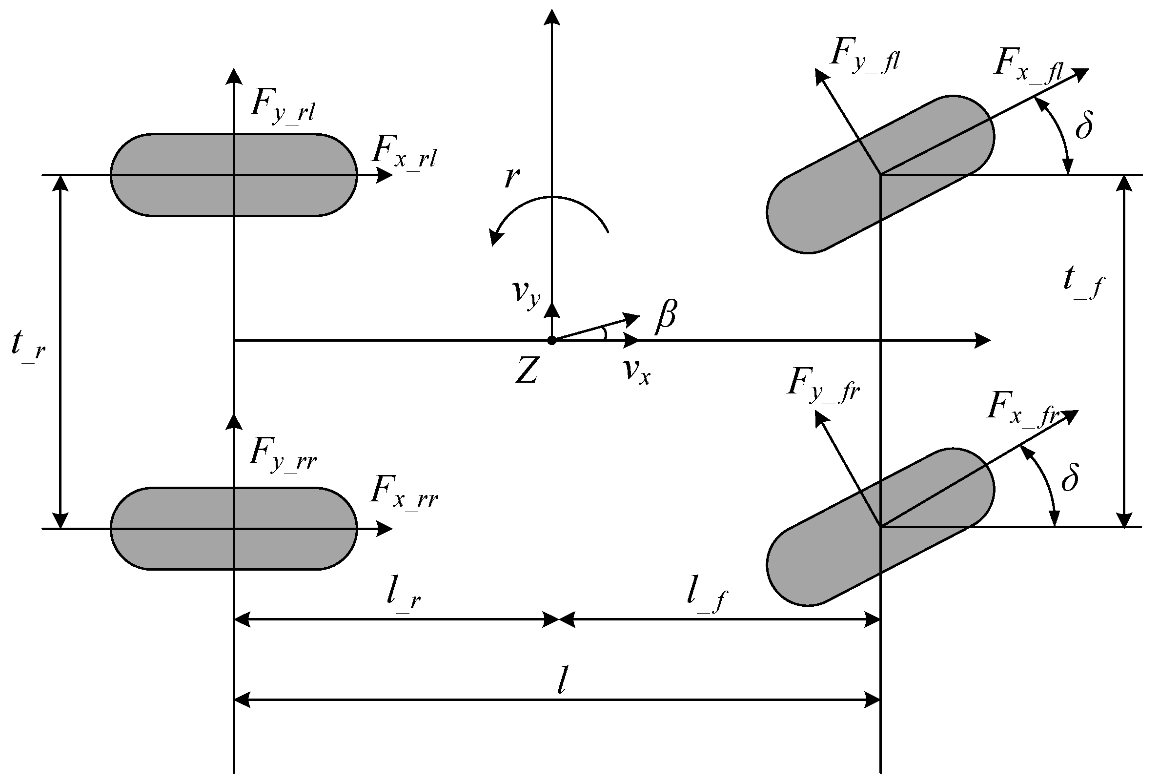
2.1. Seven-Degree-of-Freedom Vehicle Dynamics Model

In this paper, a seven-degree-of-freedom vehicle dynamics model is established, as shown in Figure 1. In order to facilitate the study, the following assumptions are made:

Figure 1. Seven-degree-of-freedom vehicle dynamics model.

a.

Ignore the impact of air resistance and suspension system;

b.

The steering angle of the front wheel is the same, and the rear wheel is not steering;

c.

The center of gravity of the vehicle coincides with the origin of the vehicle coordinate system;

d.

Do not consider the impact of roll motion on vehicle dynamics.

A seven-degree-of-freedom vehicle dynamics model including longitudinal, lateral, and yaw dynamics equations can be described as follows [19]:

Longitudinal:

$$m({\dot{v}}_x-r{v}_y)=(F_{x\_fl}+F_{x\_fr})\cos \delta -(F_{y\_fl}+F_{y\_fr})\sin \delta +F_{x\_rl}+F_{x\_rr}$$

(1)

Lateral:

$$m({\dot{v}}_y+r{v}_x)=(F_{x\_fl}+F_{x\_fr})\sin \delta +(F_{y\_fl}+F_{y\_fr})\cos \delta +F_{y\_rl}+F_{y\_rr}$$

(2)

Yaw:

$$\begin{array}{l}{I}_{zz}\cdot \dot{r}=l_{\_f}(F_{x\_fl}\sin \delta +F_{x\_fr}\sin \delta +F_{y\_fl}\cos \delta +F_{y\_fr}\cos \delta )\\ +\frac{t_{\_f}}{2}(F_{x\_fr}\cos \delta -F_{x\_fl}\cos \delta )+\frac{t_{\_f}}{2}(F_{y\_fl}\sin \delta -F_{y\_fr}\sin \delta )\\ +(F_{x\_rr}-F_{x\_rl})\frac{t_{\_r}}{2}-(F_{y\_rl}+F_{y\_rr})l_{\_r}\end{array}$$

(3)

The variables in the formula are as follows: $m$ denotes the mass of the vehicle, $a_x$ represents the longitudinal acceleration of the vehicle, and $a_y$ signifies the lateral acceleration of the vehicle. The moment of inertia around the z axis is represented by the variable $I_{zz}$. The yaw rate is denoted by the variable $r$, and the steering angle of the front wheel is represented by the variable $\delta$. The distances from the center of gravity (CG) to the front and rear axles are denoted as $l_{\_f}$ and $l_{\_r}$, respectively. The front and rear tread are denoted as $t_{\_f}$ and $t_{\_r}$, respectively. The variable $F_{x\_ij}$ denotes the longitudinal tire force, $F_{y\_ij}$ represents the lateral tire force, and $ij=[fl,fr,rl,rr]$ corresponds to the left front wheel, right front wheel, left rear wheel, and right rear wheel, respectively.

2.2. Dugoff Tire Model

The Dugoff tire model elucidates the correlation between the motion of a tire and the resulting force. The Dugoff tire model is explicated herein to aid in the development of succeeding algorithms [18]:

$$F_{x\_ij}=\mu F_{x\_ij}^0=\mu F_{z\_ij}\cdot C_{x\_ij}\frac{{\lambda }_{\_ij}}{1-{\lambda }_{\_ij}}\cdot f(L_x)$$

(4)

$$F_{y\_ij}=\mu F_{y\_ij}^0=\mu F_{z\_ij}\cdot C_{y\_ij}\frac{\tan ({\alpha }_{\_ij})}{1-{\lambda }_{\_ij}}\cdot f(L_x)$$

(5)

$$f(L_x)=\left\{\begin{array}{c}{L}_x(2-L_x),L_x<1\\ 1,L_x\ge 1\end{array}\right.$$

(6)

$$L_x=\frac{(1-{\lambda }_{\_ij})(1-\epsilon v_x\sqrt{{(C_{x\_ij}{\lambda }_{\_ij})}^2+{(C_{y\_ij}\tan {\alpha }_{\_ij})}^2})}{2\sqrt{C_{x\_ij}^2{\lambda }_{\_ij}^2+C_{y\_ij}^2{\tan }^2{\alpha }_{\_ij}}}$$

(7)

The calculation for determining the vertical tire load is as follows:

$$F_{z\_fl,fr}=mg\frac{l_{\_r}}{2l}-m{a}_x\frac{h_{cg}}{2l}\mp m{a}_y\frac{h_{cg}}{t_{\_f}}\cdot \frac{l_{\_r}}{l}$$

(8)

$$F_{z\_rl,rr}=mg\frac{l_{\_f}}{2l}+m{a}_x\frac{h_{cg}}{2l}\mp m{a}_y\frac{h_{cg}}{t_{\_r}}\cdot \frac{l_{\_f}}{l}$$

(9)

Tire sideslip angle is

$${\alpha }_{\_fl,fr}=\delta -\arctan \left(\frac{v_y+l_{\_f}r}{v_x\mp \frac{t_{\_f}}{2}r}\right)$$

(10)

$${\alpha }_{\_rl,rr}=-\arctan \left(\frac{v_y-l_{\_r}r}{v_x\mp \frac{t_{\_r}}{2}r}\right)$$

(11)

Tire slip ratio can be calculated by the following formula:

$${\lambda }_{\_ij}=\frac{R_m{w}_{ij}-v_{ij}}{\max (R_e{w}_{ij},v_{ij})}$$

(12)

The value of each wheel’s center speed is

$$v_{fl,fr}=\sqrt{{v_x}^2+{v_y}^2}+r\left(\pm \frac{t_{\_f}}{2}-l_{\_f}\beta \right)$$

(13)

$$v_{rl,rr}=\sqrt{{v_x}^2+{v_y}^2}+r\left(\pm \frac{t_{\_r}}{2}-l_{\_r}\beta \right)$$

(14)

where $\mu$ is the TRFC, $C_{x\_ij}$ and $C_{y\_ij}$ are the longitudinal stiffness and turning stiffness of the tire, respectively. $F_{z\_ij}$ is vertical tire load, $F_{x\_ij}^0$ and $F_{y\_ij}^0$ are normalized tire longitudinal force and lateral force, respectively, ${\lambda }_{\_ij}$ is tire slip ratio of four wheels, $h_{cg}$ is the height of CG, $l$ is the distance from the front axle to the rear axle, $l=l_{\_f}+l_{\_r}$, $w_{ij}$ is the wheel angular speed, and $R_m$ is the wheel rolling radius.

2.3. PMSM Mathematical Model

In this paper, a surface-mounted PMSM is selected as the drive motor of vehicle. In order to facilitate the design of speed sensorless control method for permanent magnet synchronous motor, its velocity ring siding model controller adopts the mathematical model in a $d-q$ coordinate system [19], and the rotor position and velocity observer adopts the mathematical model in an $\alpha -\beta$ coordinate system.

The mathematical expression of the PMSM in a $d-q$ coordinate system can be described as

$$\left\{\begin{array}{l}{u}_d=R{i}_d+L_s\frac{d{i}_d}{dt}-p_n{\omega }_m{L}_s{i}_q\\ u_q=R{i}_q+L_s\frac{d{i}_q}{dt}+p_n{\omega }_m{L}_s{i}_d+p_n{\omega }_m{\phi }_f\\ J\frac{d{\omega }_m}{dt}=\frac{3}{2}{p}_n{\phi }_f{i}_q-T_L\end{array}\right.$$

(15)

The mathematical expression model of the PMSM in an $\alpha -\beta$ coordinate system is given by the following formula:

$$\left\{\begin{array}{l}{u}_{\alpha }=R{i}_{\alpha }+L_s\frac{d{i}_{\alpha }}{dt}-p_n{\omega }_m{\phi }_f\sin (p_n{\theta }_m)\\ u_{\beta }=R{i}_{\beta }+L_s\frac{d{i}_{\beta }}{dt}+p_n{\omega }_m{\phi }_f\cos (p_n{\theta }_m)\\ J\frac{d{\omega }_m}{dt}=T_e-T_L-B{\omega }_m\\ {\theta }_m=\int {\omega }_{m}dt\end{array}\right.$$

(16)

where the stator voltages of the d-axis and q-axis are represented by variables $u_d$ and $u_q$, respectively. Similarly, the stator voltages of the α-axis and β-axis are represented by variables $u_{\alpha }$ and $u_{\beta }$, respectively. The stator currents for the d-axis and q-axis are represented by $i_d$ and $i_q$, respectively. Similarly, the stator currents for the α-axis and β-axis are represented by $i_{\alpha }$ and $i_{\beta }$, respectively. $R$ represents the resistance of the stator, while $L_s$ represents the inductance of the stator. The variable $p_n$ represents the number of poles, ${\omega }_m$ represents the mechanical angular speed of the rotor, and ${\theta }_m$ represents the mechanical angular position of the rotor. The variable ${\phi }_f$ represents the flux linkage of the rotor magnet, $J$ represents the moment of inertia of the rotor, $T_e$ represents the electromagnetic torque, $T_L$ represents the load torque, and $B$ represents the viscous damping.

3. MCSVDGHCKF Algorithm

The SVDGHCKF algorithm, which is based on MCC, is developed to address the issue of the HCKF algorithm being prone to divergence and non-positive definite when working with non-Gaussian noise. In a non-Gaussian noise environment, MCC can improve the estimator’s resilience and accuracy. Figure 2 illustrates the MCSVDGHCKF algorithm’s block diagram.

Figure 2. Flowchart of MCSVDGHCKF algorithm.

3.1. Maximum Correntropy Criterion

The similarity between two random variables, $X\in R$ and $Y\in R$, is measured by correlation entropy [20]. Under the assumption that their joint distribution function is $F_{XY}(x,y)$, the standard definition of the correlation entropy is

$$V(X,Y)=E[\kappa (X,Y)]=\int \kappa (x,y)d{F}_{XY}(x,y)$$

(17)

where $E[\cdot ]$ represents the expected value and $\kappa (x,y)$ is a shifted invariant kernel. The correlation entropy of the kernel function is selected to be the Gaussian kernel, i.e.,

$$\kappa (x,y)=G_{\sigma }(e)=\exp \left(-\frac{e^2}{2{\sigma }^2}\right)$$

(18)

where the correlation entropy’s nuclear bandwidth is denoted by $\sigma >0$, and $e=x-y$.

Practically speaking, there are typically only a few data samples available, and the joint distribution $F_{XY}$ is typically unknown. In this situation, we often estimate the correlation entropy using a sample mean estimator:

$$\widehat{V}(X,Y)=\frac{1}{N}{\displaystyle \sum _{i=1}^N{G}_{\sigma }(e(i))}$$

(19)

where N samples were extracted from $F_{XY}$ to form ${\{x(i),y(i)\}}_{i=1}^N$ and $e(i)=x(i)-y(i)$.

The Taylor series expansion with Gaussian nuclei results in

$$V(X,Y)={\displaystyle \sum _{n=0}^{\infty }\frac{{(-1)}^n}{2^n{\sigma }^{2n}n!}E[{(X-Y)}^{2n}]}$$

(20)

The correlation entropy is obviously the weighted sum of all the even order moments of the error variable aa, whereas the kernel bandwidth is utilized as a parameter to weigh the second and higher order moments. The second instant is important in the correlation entropy, especially when the nuclear bandwidth is big.

In heavy tail noise, the use of correlation entropy as a cost function is valid, and the associated criterion is known as MCC. If the error data series ${\{e(i)\}}_{i=1}^N$ is available, the cost function is as follows:

$$J_{MCC}=\frac{1}{N}{\displaystyle \sum _{i=1}^N{G}_{\sigma }(e(i))}$$

(21)

3.2. SVDGHCKF Algorithm Steps

$$\left\{\begin{array}{l}{x}_k=f(x_{k-1},u_{k-1})+v_{k-1}\\ z_k=h(x_k,u_k)+w_k\end{array}\right.$$

(22)

where the state vector of the system is represented by the variable $x_k\in R^n$, while the observation vector is denoted by $z_k\in R^m$. The state function of the system is given by the variable $f(\cdot )$, and the measurement function is represented by $h(\cdot )$. The variables $v_{k-1}$ and $w_k$ represent the noise in the system’s processes and measurements, respectively. Both noises are autonomous. Their covariances are $Q_{k-1}$ and $R_k$, respectively.

3.2.1. Singular Value Decomposition (SVD)

The Cholesky decomposition can yield the error covariance matrix, which is crucial for the filter method. However, if this process is stopped prematurely, it might lead to the collapse of the algorithm. This paper utilizes singular value decomposition (SVD) technology as a substitute for Cholesky decomposition in order to enhance the stability of the state parameter estimation algorithm [21].

The precise derivation is given below:

After several filters, the HCKF linear differential matrix $P_k$ gradually loses negative positive, but is still the n-level symmetric matrix, then there must be the n-level rectangular matrix V making $P_k^T{P}_k$ similar to the diagonal matrix, assuming the rank of $P_k$ is r and $0<r<n$.

$$V^T{P}_k^T{P}_{k}V=diag({\sigma }_1^2,{\sigma }_2^2,\dots ,{\sigma }_r^2,0,\dots ,0)$$

(23)

recorded as

$$S_n^2=\left[\begin{array}{cc}{S}_r^2& 0\\ 0& 0\end{array}\right]$$

(24)

$$V=[V_1,V_2]=[v_1,v_2,\dots ,v_r,v_{r+1},\dots ,v_n]$$

(25)

where ${\sigma }_1^2,{\sigma }_2^2,\dots ,{\sigma }_r^2$ is a set of orthonormal bases, i.e., there is $U_2$ such that $U=[U_1,U_2]$ is an orthonormal matrix of order n. It is calculated that

$$U_T{P}_{k}V=\left[\begin{array}{cc}{U}_1^T{P}_k{V}_1& U_1^T{P}_k{V}_2\\ U_2^T{P}_k{V}_1& U_2^T{P}_k{V}_2\end{array}\right]=\left[\begin{array}{cc}{S}_r^2& 0\\ 0& 0\end{array}\right]$$

(26)

$$P_k=U\left[\begin{array}{cc}{S}_r^2& 0\\ 0& 0\end{array}\right]V^T=U\left[\begin{array}{cc}{S}_r^2& 0\\ 0& 0\end{array}\right]U^T$$

(27)

SVD can decompose any matrix into several relatively simple matrix products, which not only retain the characteristics of the decomposed matrix, but also avoids the root operation, ensuring the numerical robustness in the iterative process.

3.2.2. Generalized Cubature Criteria

Generalized cubature rules are employed to enhance the accuracy of estimating vehicle state parameters. This improvement is achieved by enhancing the selection of cubature points and weights in the HCKF method.

The formula for generalized cubature integration is as follows [22]:

$$I(f)={\displaystyle \int {}_{R^n}f(x)\exp (-x^{T}x)}dx={\widehat{W}}_{0}f[0]+{\widehat{W}}_1{\displaystyle \sum _{i=1}^{2n}f[v]}+{\widehat{W}}_{1,1}{\displaystyle \sum _{i=1}^{2n(n-1)}f[v,v].}$$

(28)

where ${\widehat{W}}_0,{\widehat{W}}_1$ and ${\widehat{W}}_{1,1}$ are weights corresponding to $f[0],f[v],$ and $f[v,v]$ and satisfy the following formula:

$$\left[\begin{array}{c}{I}_0\\ I_2\\ I_4\\ I_{2,2}\end{array}\right]=\left[\begin{array}{c}{\widehat{W}}_0+2n{\widehat{W}}_1+2n(n-1){\widehat{W}}_{1,1}\\ 2v^2{\widehat{W}}_1+4(n-1)v^2{\widehat{W}}_{1,1}\\ 2v^2{\widehat{W}}_1+4(n-1)v^4{\widehat{W}}_{1,1}\\ 4v^4{\widehat{W}}_{1,1}\end{array}\right]$$

(29)

According to Equation (28), it can be solved as follows:

$$\left\{\begin{array}{l}{I}_0={\displaystyle \int {}_{R^n}\exp (-x^{T}x)}dx=\sqrt{{\pi }^n}\\ I_2={\displaystyle \int {}_{R^n}\exp (-x^{T}x)}dx=\sqrt{{\pi }^n}/2\\ I_4={\displaystyle \int {}_{R^n}{x}_1^4\exp (-x^{T}x)}dx=3\sqrt{{\pi }^n}/4\\ I_{2,2}={\displaystyle \int {}_{R^n}{x}_1^2{x}_2^2\exp (-x^{T}x)}dx=\sqrt{{\pi }^n}/4\end{array}\right.$$

(30)

The only solution to Equation (29) is obtained as follows:

$$\begin{array}{l}v=\sqrt{\frac{3}{2}}\\ {\widehat{W}}_0=[1-(7-n)n/18]\sqrt{{\pi }^n}\\ {\widehat{W}}_1=(4-n)\sqrt{{\pi }^n}/18;{\widehat{W}}_2=\sqrt{{\pi }^n}/36.\end{array}$$

(31)

Substituting the result of the above formula into Equation (27), we can get

$$\begin{array}{ll}I(f)& ={\displaystyle \int {}_{R^n}f(x)\exp (-x^{T}x)}\\ & =\left(1-\frac{(7-n)n}{18}\right)f([0])+\frac{4-n}{18}{\displaystyle \sum _{i=1}^{2n}f({[\sqrt{3}]}_i})+\frac{1}{36}{\displaystyle \sum _{i=1}^{2n(n-1)}f({[\sqrt{3},\sqrt{3}]}_i)}.\end{array}$$

(32)

The calculation of the filter weights and cubature points can be performed using Equations (33) and (34).

$$W_i=\left\{\begin{array}{l}1-(7-n)n/18,i=1\\ (4-n)/18,i=2,\dots ,2n+1\\ 1/36,i=2n+2,\dots ,2n^2+1\end{array}\right.$$

(33)

$${\xi }_i=\left\{\begin{array}{l}{[0]}_i,i=1\\ {[\sqrt{3}]}_i,i=2,\dots ,2n+1\\ {[\sqrt{3},\sqrt{3}]}_i,i=2n+2,\dots ,2n^2+1\end{array}\right.$$

(34)

3.2.3. SVDGHCKF Algorithm

Predict:

(1)

Cubature point propagation:

$$x_{i,k-1}=x_{k-1}+U_{k-1}\left[\begin{array}{cc}\sqrt{S_{k-1}}& 0\\ 0& 0\end{array}\right]{\xi }_i,i=1,\dots ,2n^2+1$$

(35)

(2)

Following propagation, the cubature points are as follows:

$$x_{i,k|k-1}^{*}=f(x_{i,k-1},u_{k-1})$$

(36)

(3)

The predicted value of the state is given by the following formula:

$${\widehat{x}}_{k|k-1}={\displaystyle \sum _{i=1}^{2n^2+1}{W}_i{x}_{i,k|k-1}^{*}}$$

(37)

(4)

Calculate the covariance matrix for the state prediction at the k + 1 moment:

$$P_{k|k-1}={\displaystyle \sum _{i=1}^{2n^2+1}{W}_i}(x_{i,k|k-1}^{*}-{\widehat{x}}_{k|k-1}){(x_{i,k|k-1}^{*}-{\widehat{x}}_{k|k-1})}^T+Q_{k-1}$$

(38)

Update:

(1)

Update the status cubature points as follows:

$$x_{i,k|k-1}=U_k\left[\begin{array}{cc}\sqrt{S_k}& 0\\ 0& 0\end{array}\right]{\xi }_i+{\widehat{x}}_{k|k-1},i=1,\dots ,2n^2+1$$

(39)

(2)

The cubature points transmitted by the measuring equation are provided as follows:

$$z_{i,k}=h(x_{i,k},u_k)$$

(40)

(3)

The measured predicted values are as follows:

$${\widehat{z}}_k={\displaystyle \sum _{i=1}^{2n^2+1}{W}_i{z}_{i,k}}$$

(41)

(4)

The measurement error covariance matrix and cross-correlation covariance matrix are provided in the following manner:

$$\begin{array}{l}{P}_k^{zz}=z_k{z}_k^T+R_k\\ P_{k|k-1}^{xz}=x_{k|k-1}{z}_k^T\end{array}$$

(42)

(5)

The expression for the Kalman filter gain is as follows:

$$K_k=P_{k|k-1}^{xz}{(P_k^{zz})}^{-1}$$

(43)

(6)

State estimates are given as follows:

$${\widehat{x}}_k={\widehat{x}}_{k|k-1}+K_k(z_k-{\widehat{z}}_k)$$

(44)

(7)

The matrix representing the covariance of the posterior distribution is given by the following equation:

$$P_k=P_{k|k-1}-K_k(P_k^{zz})K_k^T$$

(45)

3.3. Derivation of the MCSVDGHCKF

MCC is resistant in the presence of non-Gaussian noise because the correlation entropy incorporates the second and higher moments of the error [23]. MCC is used in this section to improve the robustness of the SVDGHCKF.

Then, according to Equation (22), the following nonlinear regression model is constructed:

$$\left[\begin{array}{c}{\widehat{x}}_{k|k-1}\\ z_k\end{array}\right]=\left[\begin{array}{c}{x}_k\\ h(x_k,u_k)\end{array}\right]+{\varphi }_k$$

(46)

where $\varphi (k)=\left[\begin{array}{c}{\widehat{x}}_{k|k-1}-x_k\\ w_k\end{array}\right]$.

According to Equation (38), the covariance of matrix ${\varphi }_k$ can be written as

$$E[{\varphi }_k{\varphi }_k^T]=\left[\begin{array}{cc}{P}_{k|k-1}& 0\\ 0& R_k\end{array}\right]=\left[\begin{array}{cc}{M}_{p,k|k-1}& 0\\ 0& M_{r,k}{M}_{r,k}^T\end{array}\right]=M_k{M}_k^T$$

(47)

where we may obtain $M_{p,k|k-1}$, $M_{r,k}$, and $M_k$ by performing the Cholesky decomposition on $M_{p,k|k-1}$.

Multiply the left side of both sides of the Equation (47) by $M_k^{-1}$ to get

$$D_k=g(x_k,u_k)+e_k$$

(48)

where $D_k=M_k^{-1}\left[\begin{array}{c}{\widehat{x}}_{k|k-1}\\ z_k\end{array}\right]$,$g(x_k,u_k)=M_k^{-1}\left[\begin{array}{c}{x}_k\\ h(x_k,u_k)\end{array}\right]$, and $e_k=M_k^{-1}{\varphi }_k$.

The cost function is given by the following formula using Equation (48) and MCC:

$$J_{MCC}(x_k)={\displaystyle \sum _{i=1}^{n+m}{G}_{\sigma }(e_{i,k})={\displaystyle \sum _{i=1}^{n+m}{G}_{\sigma }(d_{i,k}-g_i(x_k,u_k))}}$$

(49)

Here, $d_{i,k}$ represents the i-th element of $D_k$, and $g_i(x_k,u_k)$ represents the i-th row of $g(x_k,u_k)$.

The solution for $x_k$ under MCC is then expressed as follows:

$${\widehat{x}}_k=\underset{x_k}{\arg \max }{\displaystyle \sum _{i=1}^{n+m}{G}_{\sigma }(e_{i,k})}$$

(50)

If the value of Equation (50) is zero, the optimal solution for $x_k$ can be obtained by

$$\frac{\partial J_{MCC}(x_k)}{\partial x_k}={\displaystyle \sum _{i=1}^{n+m}{G}_{\sigma }(e_{i,k})\cdot }{e}_{i,k}\cdot \frac{\partial e_{i,k}}{\partial x_k}=0$$

(51)

By defining $C_{i,k}=G_{\sigma }(e_{i,k})$, we can get

$$C_k=diag(G_{\sigma }(e_{i,k}),\dots ,G_{\sigma }(e_{n+m,k}))=\left[\begin{array}{cc}{C}_{x,k}& 0\\ 0& C_{y,k}\end{array}\right]$$

(52)

where $C_{x,k}=\left[\begin{array}{ccc}{G}_{\sigma }(e_{1,k})& \cdots & 0\\ ⋮& \ddots & ⋮\\ 0& \cdots & G_{\sigma }(e_{n,k})\end{array}\right],C_{y,k}=\left[\begin{array}{ccc}{G}_{\sigma }(e_{n+1,k})& \cdots & 0\\ ⋮& \ddots & ⋮\\ 0& \cdots & G_{\sigma }(e_{n+m,k})\end{array}\right]$, diag(·) represents the operation of establishing a diagonal matrix.

It can be further expressed using Equations (51) and (52) as follows:

$${\left(\frac{\partial g(x_k,u_k)}{\partial x_k}\right)}^T{C}_k(D_k-g(x_k,u_k))=0$$

(53)

Updating the state covariance and measuring the noise variance through $C_k$ are the two main components of employing MCC to improve the performance of the SVDGHCKF with non-Gaussian noise. As a result, we define ${\tilde{L}}_{k|k}$ as the update covariance matrix of ${\varphi }_k$.

$${\tilde{L}}_{k|k}=\left[\begin{array}{cc}{\tilde{P}}_{k|k-1}& 0\\ 0& {\tilde{R}}_k\end{array}\right]=M_k\cdot C_k^{-1}\cdot M_k^T$$

(54)

In fact, since we have no way of knowing the true state $x_k$, let $x_k={\widehat{x}}_{k|k-1}$. Thus, the prior state covariance and noise covariance can be written as

$${\tilde{P}}_{k|k-1}=M_{p,k|k-1}\cdot I\cdot M_{p,k|k-1}^T$$

(55)

$${\tilde{R}}_k=M_{r,k}{C}_{y,k}^{-1}{M}_{r,k}^T$$

(56)

Finally, we incorporate the prior state covariance and measurement noise covariance updating processes into the SVDGHCKF algorithm to obtain the MCSVDGHCKF algorithm.

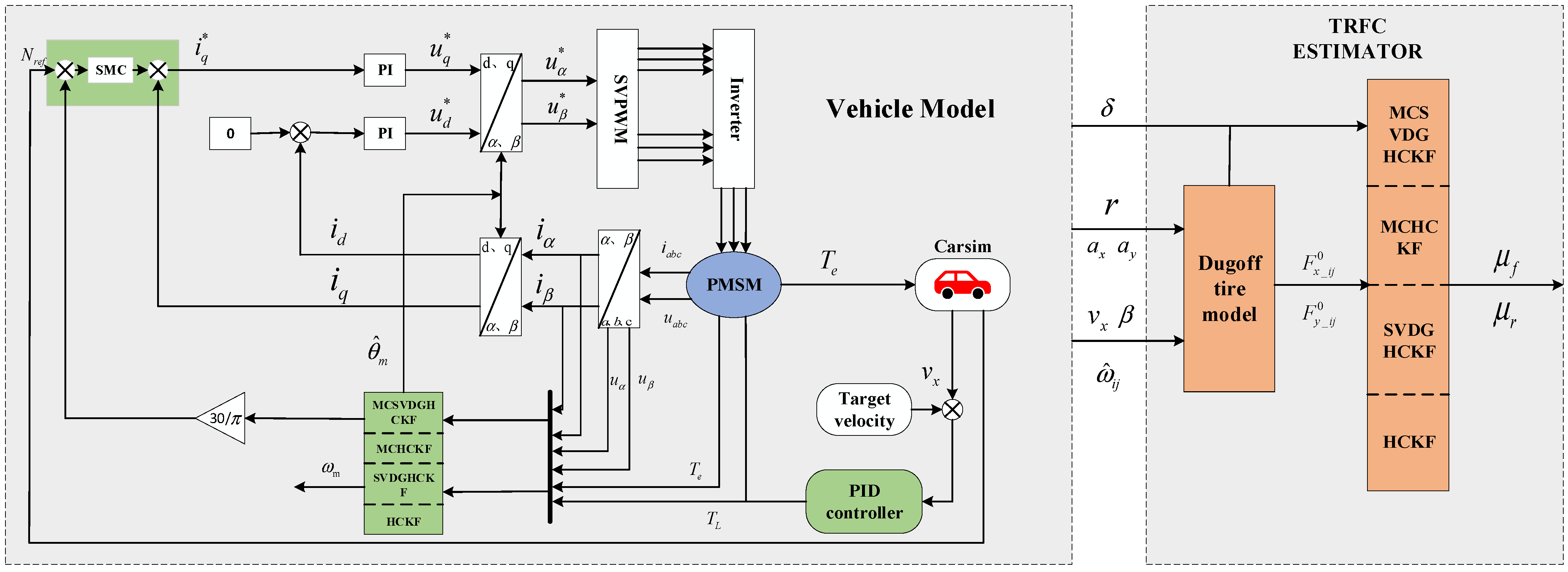
4. TRFC Estimation for Sensorless Control of PMSM

The TRFC estimate technique, which utilizes PMSM sensorless control, is seen in Figure 3. A model of a distributed drive electric vehicle (DDEV) was created using Carsim/Simulink. In Figure 3, a single-wheel motor was chosen to demonstrate the concept. The load torque of the PMSM $T_L$ is determined by calculating the difference between the actual vehicle speed and the target vehicle speed using the SMC controller, with the output speed of Carsim being considered as the actual vehicle speed. The wheel angular speed outputted by Carsim serves as the reference speed $N_{ref}$ for the PMSM. The PMSM generates the electromagnetic torque $T_e$, which serves as the driving force for the wheel. The MCSVDGHCKF technique is utilized to estimate the rotor speed, which is then employed as the input wheel angular speed for the Dugoff tire model. Subsequently, the normalized tire force is incorporated into the TRFC estimator based on the MCSVDGHCKF.

Figure 3. TRFC estimation scheme based on sensorless control of PMSM.

4.1. PMSM Rotor Speed and Position Estimator Based on MCSVDGHCKF

A discrete mathematical model of a PMSM is developed in this study. The MCSVDGHCKF algorithm is employed to accurately determine the speed and position of the PMSM rotor. By converting the mathematical representation of a permanent magnet synchronous motor (PMSM) from the α-β coordinate system to the state space form [19], we obtain

$$\left\{\begin{array}{l}{\dot{x}}_1=A{x}_1+B{u}_1+w_1\\ z_1=C{x}_1+v_1\end{array}\right.$$

(57)

$$x_1=\left[\begin{array}{c}{i}_{\alpha }\\ i_{\beta }\\ {\omega }_m\\ {\theta }_m\end{array}\right],z_1=\left[\begin{array}{c}{i}_{\alpha }\\ i_{\beta }\end{array}\right],u_1=\left[\begin{array}{c}{u}_{\alpha }\\ u_{\beta }\\ T_e\\ T_L\end{array}\right]$$

(58)

where $x_1$ is the state vector, $u_1$ is the control input, and $z_1$ is the direction-finding quantity.

$$A=\left[\begin{array}{cccc}-\frac{R}{L_s}& 0& \frac{p_n{\phi }_f}{L_s}\sin (p_n{\theta }_m)& 0\\ 0& -\frac{R}{L_s}& -\frac{p_n{\phi }_f}{L_s}\cos (p_n{\theta }_m)& 0\\ 0& 0& -\frac{R}{J}& 0\\ 0& 0& 1& 0\end{array}\right]$$

(59)

$$B=\left[\begin{array}{cccc}\frac{1}{L_s}& 0& 0& 0\\ 0& \frac{1}{L_s}& 0& 0\\ 0& 0& \frac{1}{J}& -\frac{1}{J}\\ 0& 0& 0& 0\end{array}\right],C=\left[\begin{array}{cccc}1& 0& 0& 0\\ 0& 1& 0& 0\end{array}\right]$$

(60)

Using the Euler discretization method we discretize a PMSM mathematical model

$$\left\{\begin{array}{l}{x}_{1,k}=F_1{x}_{1,k-1}+G{u}_{1,k-1}+v_{1,k-1}\\ z_{1,k}=H_1{x}_{1,k}+w_{1,k}\end{array}\right.$$

(61)

where

$$\begin{array}{ll}{F}_1& =I+AT\\ & =\left[\begin{array}{cccc}1-\frac{R}{L_s}& 0& \frac{T{p}_n{\phi }_f}{L_s}\sin (p_n{\theta }_m)& 0\\ 0& 1-\frac{R}{L_s}& -\frac{T{p}_n{\phi }_f}{L_s}\cos (p_n{\theta }_m)& 0\\ 0& 0& 1-\frac{R}{J}& 0\\ 0& 0& T& 0\end{array}\right]\end{array}$$

(62)

$$G=BT=\left[\begin{array}{cccc}\frac{T}{L_s}& 0& 0& 0\\ 0& \frac{T}{L_s}& 0& 0\\ 0& 0& \frac{T}{J}& -\frac{T}{J}\\ 0& 0& 0& 0\end{array}\right]$$

(63)

$$H_1=C=\left[\begin{array}{cccc}1& 0& 0& 0\\ 0& 1& 0& 0\end{array}\right]$$

(64)

Based on the MCSVDGHCKF algorithm, the PMSM discrete mathematical model established by Equations (61)–(64) can be used to estimate rotor speed and position.

4.2. TRFC Estimator Based on MCSVDGHCKF

The Carsim software was used to gather data from various sources, including front wheel steering angle, yaw rate, longitudinal acceleration, lateral acceleration, longitudinal speed, vehicle sideslip angle, and estimated rotor speed. This data was then inputted into the Dugoff tire model to calculate the normalized tire force. Additionally, a TRFC estimator was developed using the MCSVDGHCKF algorithm, which utilizes the relationship between TRFC and tire force.

According to the relationship between $F_{x\_ij}$ and $F_{x\_ij}^0$ and between $F_{y\_ij}$ and $F_{y\_ij}^0$ in Equations (4) and (5), the discrete mathematical model can be derived from Equations (1)–(3) in the following manner:

$$x_{2,k}=F_2{x}_{2,k-1}+v_{2,k-1}$$

(65)

$$F_2=\left[\begin{array}{cccc}1+T& 0& 0& 0\\ 0& 1+T& 0& 0\\ 0& 0& 1+T& 0\\ 0& 0& 0& 1+T\end{array}\right]$$

(66)

$$\begin{array}{l}{z}_{2,k}=h(x_{2,k},u_{2,k})+w_{2,k}\\ {\left[\begin{array}{c}{a}_x\\ a_y\\ \dot{r}\end{array}\right]}_k={\left[\begin{array}{cccc}{h}_{1,1}& h_{1,2}& h_{1,3}& h_{1,4}\\ h_{2,1}& h_{2,2}& h_{2,3}& h_{2,4}\\ h_{3,1}& h_{3,2}& h_{3,3}& h_{3,4}\end{array}\right]}_k\left[\begin{array}{c}{\mu }_{fl}\\ {\mu }_{fr}\\ {\mu }_{rl}\\ {\mu }_{rr}\end{array}\right]+w_{2,k}\end{array}$$

(67)

$$\begin{array}{l}{h}_{1,1}=\frac{F_{x\_fl}^0\cos \delta -F_{y\_fl}^0\sin \delta }{m},h_{1,2}=\frac{F_{x\_fr}^0\cos \delta -F_{y\_fr}^0\sin \delta }{m}\\ h_{1,3}=\frac{F_{x\_rl}^0}{m},h_{1,4}=\frac{F_{x\_rr}^0}{m}\end{array}$$

(68)

$$\begin{array}{l}{h}_{2,1}=\frac{F_{x\_fl}^0\sin \delta +F_{y\_fl}^0\cos \delta }{m},h_{2,2}=\frac{F_{x\_fr}^0\sin \delta -F_{y\_fr}^0\cos \delta }{m}\\ h_{2,3}=\frac{F_{y\_rl}^0}{m},h_{2,4}=\frac{F_{y\_rr}^0}{m}\end{array}$$

(69)

$$\begin{array}{l}{h}_{3,1}=\frac{l_{\_f}(F_{x\_fl}^0\sin \delta +F_{y\_fl}^0\cos \delta )-\frac{t_{\_f}}{2}(F_{x\_fl}^{0}cos\delta -F_{y\_fl}^0\sin \delta )}{I_{zz}}\\ h_{3,2}=\frac{l_{\_f}(F_{x\_fr}^0\sin \delta +F_{y\_fr}^0\cos \delta )+\frac{t_{\_f}}{2}(F_{x\_fr}^{0}cos\delta -F_{y\_fr}^0\sin \delta )}{I_{zz}}\\ h_{3,3}=\frac{-\frac{t_{\_r}}{2}{F}_{x\_rl}^0-l_{\_r}{F}_{y\_rl}^0}{I_{zz}},h_{3,4}=\frac{\frac{t_{\_r}}{2}{F}_{x\_rr}^0-l_{\_r}{F}_{y\_rr}^0}{I_{zz}}\end{array}$$

(70)

where the state vector $x_2={[{\mu }_{fl},{\mu }_{fr},{\mu }_{rl},{\mu }_{rr}]}^T$, the control input $u_2={[\delta ,F_{x\_ij}^0,F_{y\_ij}^0]}^T$, and the measurement vector $z_2={[a_x,a_y,\dot{r}]}^T$. The estimation of the TRFC can be derived by the utilization of a discrete mathematical model constructed from Equations (65)–(70), employing the MCSVDGHCKF algorithm.

4.3. Design of PMSM Speed Loop Controller Based on Sliding Mode

The vector control of the permanent magnet synchronous motor is achieved by employing the rotor magnetic field directional control method with id = 0. Therefore, Equation (15) can be rephrased as follows:

$$\left\{\begin{array}{l}\frac{d{i}_q}{dt}=\frac{1}{L_s}(-R{i}_q-p_n{\phi }_f{\omega }_m+u_q)\\ \frac{d{\omega }_m}{dt}=\frac{1}{J}(\frac{3}{2}{p}_n{\phi }_f{i}_q-T_L)\end{array}\right.$$

(71)

The PMSM system state vector is defined as

$$\left\{\begin{array}{l}{x}_1={\omega }_{ref}-{\omega }_m\\ x_2={\dot{x}}_1=-{\dot{\omega }}_m\end{array}\right.$$

(72)

where ${\omega }_{ref}$ is the motor reference angular speed.

$$\left\{\begin{array}{l}{\dot{x}}_1=\frac{1}{J}(T_L-\frac{3}{2}{p}_n{\phi }_f{i}_q)\\ {\dot{x}}_2=\frac{3p_n{\phi }_f}{2J}{\dot{i}}_q\end{array}\right.$$

(73)

Set $u={\dot{i}}_q,D=\frac{3p_n{\psi }_f}{2J}$; Equation (73) can be transformed into

$$\left[\begin{array}{l}{\dot{x}}_1\\ {\dot{x}}_2\end{array}\right]=\left[\begin{array}{cc}0& 1\\ 0& 0\end{array}\right]\left[\begin{array}{l}{x}_1\\ x_2\end{array}\right]+\left[\begin{array}{c}0\\ -D\end{array}\right]u$$

(74)

Set the sliding mode surface function and derive it:

$$\begin{array}{l}s=c{x}_1+x_2\\ \dot{s}=c{\dot{x}}_1+{\dot{x}}_2=c{x}_2-Du\end{array}$$

(75)

The expression of the sliding mode controller based on exponential reach rate is as follows:

$$u=\frac{1}{D}[c{x}_2+\epsilon \mathrm{sgn}(s)+qs]$$

(76)

Thus, the reference current of the q-axis is

$$i_q=\frac{2J}{3p_n{\psi }_f}{\displaystyle {\int }_0^t[c{x}_2+\epsilon \mathrm{sgn}(s)+qs]}d\tau$$

(77)

The Lyapunov function is chosen to prove the stability of the system as follows:

$$V(t)=\frac{1}{2}{s}^2$$

(78)

A further derivation of the above formula is

$$\dot{V}(t)=s\dot{s}=-\epsilon \left|s\right|-q{s}^2\le 0$$

(79)

It can be seen from Equation (79) that the system satisfies the stability condition.

5. Simulation Analysis

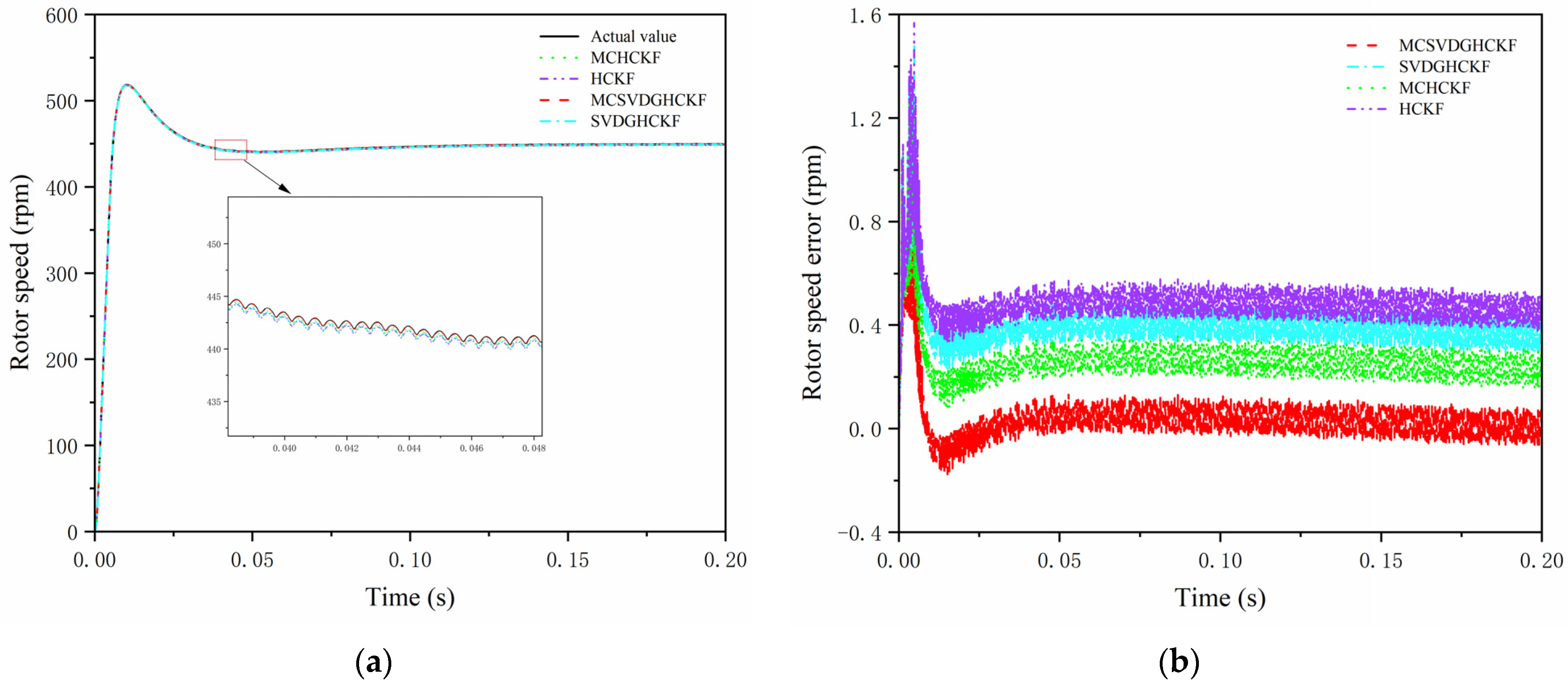
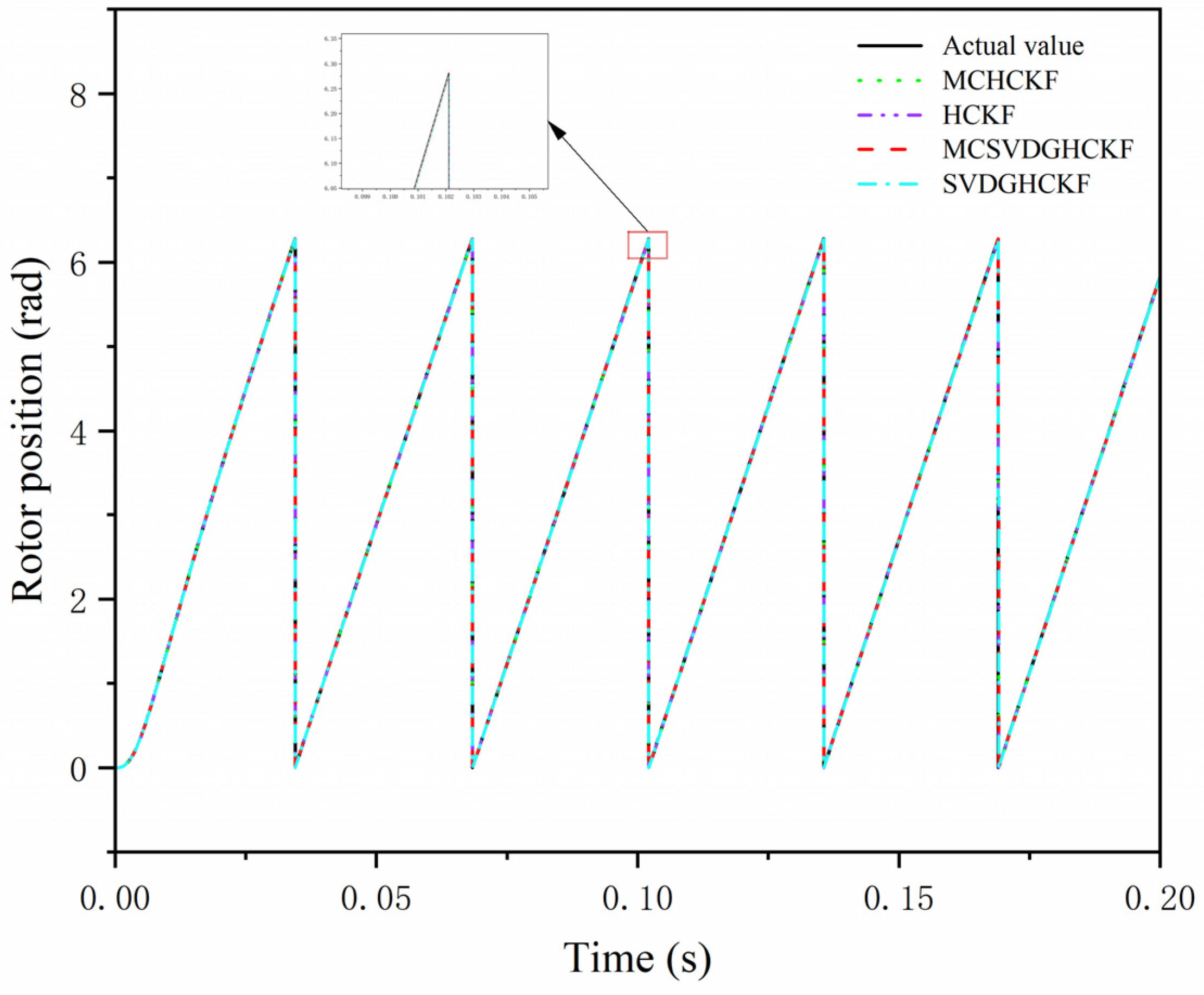
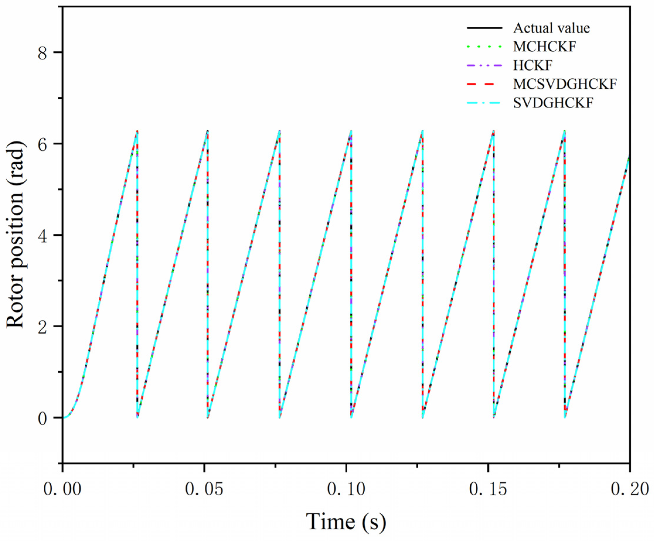
5.1. PMSM Sensorless Control Simulation and Analysis

A combined simulation was conducted in Simulink/Carsim software to validate the efficacy of the sensorless control approach for a PMSM using the MCSVDGHCKF algorithm. In this paper, the kernel width of the MCSVDGHCKF algorithm is set to $\sigma =8$. Figure 4 shows the setting of DDEV in the Carsim powertrain. The Carsim output wheel angular speed is used as a reference rotor speed. The main parameters of PMSM in simulation are shown in Table 1.

Figure 4. Carsim drivetrain setup.

Table 1. Basic parameters of PMSM.

Parameter	Value	Unit
Pole pairs (Pn)	4
Stator inductance (Ls)	0.00525	mH
Stator resistance (R)	0.958	$\Omega$
Flux linkage (${\phi }_f$)	0.1827	Wb
Rotor’s moment of inertia (J)	0.003	Kgm2
Viscous damping (B)	0.008	Nms

Figure 5 and Figure 6 display the comparison curves of rotor speed and position estimated by several comparison algorithms and the MCSVDGHCKF method at a speed of 60 km/h under serpentine conditions. The speed loop is regulated by the SMC controller. During the transition from zero rotor speed to the reference speed phase, both the rotor speed and position error experience an increase, followed by rapid stabilization. This behavior demonstrates the algorithms’ ability to respond quickly and accurately track the desired speed. The velocity estimation error comparison curve in Figure 5b demonstrates that the MCSVDGHCKF algorithm has a notably superior estimate accuracy compared to other algorithms. This is due to its ability to overcome the challenges of non-local sampling and divergence in high-dimensional systems.

Figure 5. PMSM velocity estimation and estimated error curve under serpentine conditions. (a) Rotor speed estimate; (b) rotor speed estimate error.

Figure 6. PMSM rotor position estimation under serpentine conditions.

Figure 7 and Figure 8 show the comparison curves of rotor speed and position estimated by different comparison algorithms and the MCSVDGHCKF algorithm under a step condition of 80 km/h. Under the step condition of a higher speed and faster steering wheel change, the MCSVDGHCKF has better estimation accuracy and robustness than MCHCKF, SVDGHCKF, and HCKF. The MCSVDGHCKF shows good performance in non-local sampling and divergence of high dimensional systems for PMSM state estimation.

Figure 7. PMSM velocity estimation and estimated error curve under step conditions. (a) Rotor speed estimate; (b) rotor speed estimate error.

Figure 8. PMSM rotor position estimation under step conditions.

5.2. Simulation of TRFC Estimation Using PMSM Sensorless Control

The TRFC value set in Carsim is used as the true value to test the efficacy of the algorithm for predicting the TRFC of DDEV utilizing sensorless control of a PMSM. The MCSVDGHCKF algorithm, which is based on sensorless PMSM control, is compared to the TRFC estimation algorithms MCHCKF, SVDGHCKF, and HCKF. Table 2 shows the major parameters of the Carsim car model utilized in the simulation. In this paper, the RMSE is selected as the evaluation index, and the evaluation formula is shown as follows (80):

$$RMSE=\sqrt{\frac{1}{n}{\displaystyle \sum _{k=1}^n{(x_k-{\widehat{x}}_k)}^2}}$$

(80)

Table 2. Basic parameters of DDEV.

Parameter	Value	Unit
Vehicle mass (m)	1765	kg
Yaw moment of inertia (Izz)	2700	Kgm2
Distance from the front axle to the CG (l_f)	1.2	m
Distance from the rear axle to the CG (l_r)	1.4	m
Front wheel tread (t_f)	1.6	m
Rear wheel tread (t_r)	1.6	m
Effective rolling radius of the tire (Rm)	0.354	m
Height of CG (hcg)	0.5	m

As the sensor noise is strongly influenced by the noise covariance matrix of the estimator, it is crucial to modify the estimator’s covariance prior to conducting the simulation experiment. This work examines the performance of the filter by incorporating non-Gaussian noise, aiming to simulate a real sensor data acquisition system more accurately. The covariance matrix of the process function and measurement function of the TRFC estimator is shown in Equation (81) below:

$$\left\{\begin{array}{l}{Q}_{{\mu }_{fl}}={10}^{-1}\\ Q_{{\mu }_{fr}}={10}^{-1}\\ Q_{{\mu }_{rl}}={10}^{-1}\\ Q_{{\mu }_{rr}}={10}^{-1}\\ R_{a_x}=0.0028v_k\sim 0.08N(0,0.01)+0.02N(0,0.1)\\ R_{\dot{\gamma }}=0.0028v_k\sim 0.08N(0,0.01)+0.02N(0,0.1)\\ R_{a_y}=0.0028v_k\sim 0.08N(0,0.01)+0.02N(0,0.1)\end{array}\right.$$

(81)

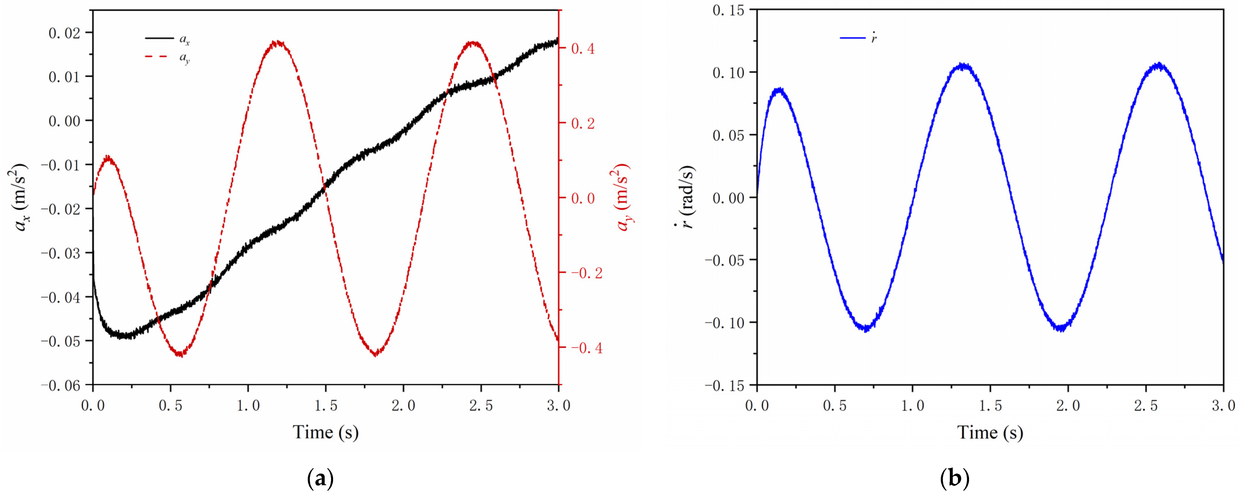
5.2.1. Serpentine Conditions

Simulation verification of serpentine steering driving with constant TRFC: Under the serpentine steering driving conditions, the TRFC in Carsim is set to 0.85, and the longitudinal speed of the vehicle is stable at 60 km/h. The measured values of the sensor are shown in Figure 9. This paper takes the right front wheel and the left rear wheel as an example to compare and analyze the TRFC estimation results under the four algorithms, and the results are shown in Figure 10 and Figure 11 and in Table 3.

Figure 9. The measured value of the sensor under serpentine conditions. (a) Longitudinal and lateral acceleration measurements; (b) yaw rate measurements.

Figure 10. Estimated TRFC of the right front wheel and estimated error curve under serpentine conditions. (a) Right front wheel TRFC estimate; (b) right front wheel TRFC estimate error.

Figure 11. Estimated TRFC of the left rear wheel and estimated error curve under serpentine conditions. (a) Left rear wheel TRFC estimate; (b) left rear wheel TRFC estimate error.

Table 3. Comparison of RMSE of vehicle parameter estimation under serpentine conditions.

Estimated Objects	Algorithm
	MCSVDGHCKF	MCHCKF	SVDGHCKF	HCKF
${\mu }_{fr}$	0.0129	0.0220	0.0246	0.0263
${\mu }_{rl}$	0.0228	0.0384	0.0410	0.0425

Figure 10 and Figure 11 show the simulation results of steering drive conditions with a constant friction coefficient. As can be seen from Figure 10a and Figure 11a, although there is a certain overshoot in the initial stage, all four algorithms can converge to the set value within 0.5 s, and the error after stabilization is less than 0.015. When a PMSM is used for sensorless control, MCHCKF has higher accuracy and faster response than SVDGHCKF and HCKF, reflecting the advantages of MCC in non-Gaussian noise environments, while MCSVDGHCKF has the smallest overshoot at the beginning and the fastest convergence to the true value. As can be seen from Figure 10b and Figure 11b and Table 3, the overall accuracy of MCSVDGHCKF estimation is higher than that of MCHCKF, SVDGHCKF and HCKF; the RMSE of TRFC estimates for the right front wheel and the left rear wheel reduced by at least 41.36% and 40.63%, indicating that MCSVDGHCKF has higher estimation accuracy and stronger robustness in non-Gaussian heavy-tail noise environment, and can adapt to harsh high-dimensional systems.

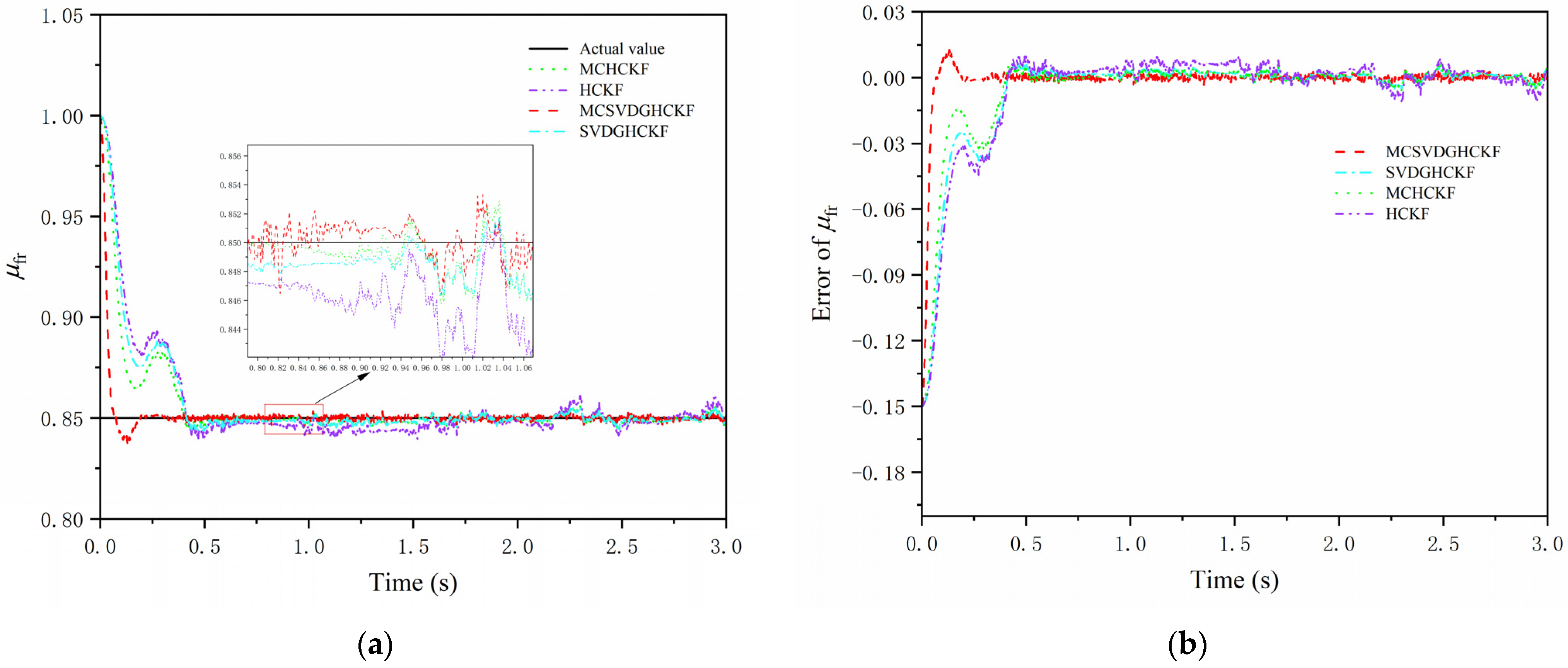
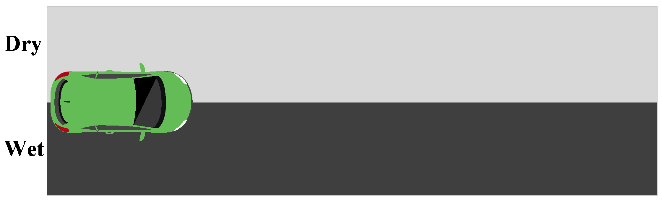
5.2.2. Step Conditions

Simulation verification of step-steering driving with a constant TRFC steering wheel angle: Under the driving conditions of step-steering at a 45° steering wheel angle, the TRFC in Carsim is set to the bisectional road surface of 0.65 and 0.3. The situation of the opposite road surface is shown in Figure 12, the vehicle speed is stable at 80 km/h, and the measured values of the sensor are shown in Figure 13. This paper takes the right front wheel and the left rear wheel as an example to compare and analyze the TRFC estimation results under the four algorithms, and the results are shown in Figure 14 and Figure 15 and Table 4.

Figure 12. Schematic diagram of the bisectional test path.

Figure 13. Sensor measurement under step conditions. (a) Longitudinal and lateral acceleration measurements; (b) yaw rate measurements.

Figure 14. Estimated TRFC of the right front wheel and estimated error curve under step conditions. (a) Right front wheel TRFC estimate; (b) right front wheel TRFC estimate error.

Figure 15. Estimated TRFC of the left rear wheel and estimated error curve under step conditions. (a) Left rear wheel TRFC estimate; (b) left rear wheel TRFC estimate error.

Table 4. Comparison of RMSE of vehicle parameter estimation under step conditions.

Estimated Objects	Algorithm
	MCSVDGHCKF	MCHCKF	SVDGHCKF	HCKF
${\mu }_{fr}$	0.0344	0.0623	0.0708	0.0730
${\mu }_{rl}$	0.0893	0.1928	0.2111	0.2166

Figure 12 and Figure 13 show the simulation results of the TRFC on the open road. As can be seen from Figure 14a, when the vehicle is driving on the right side of the low-friction road surface, the four algorithms all have a certain overshoot at the beginning stage, but the MCSVDGHCKF algorithm has a small adjustment range and a faster response to stabilization. As can be seen from Figure 15a, when the left side of the vehicle is driving on a road surface with a high friction coefficient, the four algorithms all respond quickly to sudden state changes, but after the sudden change stage, the accuracy of the MCSVDGHCKF algorithm is higher than that of the other three algorithms. As can be seen from Figure 14b and Figure 15b and Table 4, compared with SVDGHCKF, HCKF, and MCHCKF, the RMSE of the TRFC estimates for the right front wheel and the left rear wheel reduced by at least 44.78% and 53.68%, respectively. The MCSVDGHCKF algorithm has a higher estimation accuracy and stronger robustness in non-Gaussian heavy-tail noise environments, which can significantly improve the performance of the estimator in harsh high-dimensional systems.

6. Conclusions and Future Work

(1)

Aiming at the problem of low accuracy and poor robustness of TRFC estimation in non-Gaussian heavy-tail noise environments, this paper proposes a MCSVDGHCKF algorithm, which can solve the problems of HCKF divergence and non-positive definite in high-dimensional systems, and improve the accuracy and robustness of the estimator.

(2)

A sensorless control system for PMSMs is developed, employing the SMC control strategy. The utilization of the estimated rotor speed is employed in lieu of the information from the wheel angular speed sensor, and a TRFC estimation algorithm is formulated based on sensorless control of a PMSM. The efficacy of the suggested algorithm is validated by simulation studies.

(3)

In subsequent investigations, the authors intend to extend the scope of the proposed algorithm by including the roll and pitch motions of the vehicle.

References

- Shi, Y.; Li, B.; Luo, J.; Yu, F. A practical identifier design of road variations for anti-lock brake system. Veh. Syst. Dyn. 2019, 57, 336–368. [Google Scholar] [CrossRef]
- Zhang, R.; Shi, P.; Zhao, L.; Gao, Z. Research on coordinated control of electronic stability program and active suspension system based on function allocation and multi-objective fuzzy decision. Proc. Inst. Mech. Eng. Part. I J. Syst. Control Eng. 2018, 232, 1155–1169. [Google Scholar]
- Wu, X.; Zhou, B.; Wu, T.; Pan, Q. Research on intervention criterion and stability coordinated control of AFS and DYC. Int. J. Veh. Des. 2023, 90, 116–141. [Google Scholar] [CrossRef]
- Wang, Y.; Geng, K.; Xu, L.; Ren, Y.; Dong, H.; Yin, G. Estimation of sideslip angle and tire cornering stiffness using fuzzy adaptive robust cubature kalman filter. IEEE Trans. Syst. Man. Cybern. Syst. 2022, 52, 1451–1462. [Google Scholar] [CrossRef]
- Zhang, Y.; Zhang, Y.; Ai, Z.; Feng, Y.; Zhang, J.; Murphey, Y. Estimation of electric mining haul trucks’ mass and road slope using dual level reinforcement estimator. IEEE Trans. Veh. Technol. 2019, 68, 10627–10638. [Google Scholar] [CrossRef]
- Leng, B.; Jin, D.; Xiong, L.; Ying, X.; Yu, Z. Estimation of tire-road peak adhesion coefficient for intelligent electric vehicles based on camera and tire dynamics information fusion. Mech. Syst. Signal Process. 2021, 150, 107275. [Google Scholar] [CrossRef]
- Liu, F.; Wu, Y.; Yang, X.; Mo, Y.; Liao, Y. Identification of winter road friction coefficient based on multi-task distillation attention network. Pattern Anal. Appl. 2022, 25, 441–449. [Google Scholar] [CrossRef]
- Wu, Y.; Li, G.; Fan, D. Joint Estimation of Driving State and Road Adhesion Coefficient for Distributed Drive Electric Vehicle. IEEE Access 2021, 9, 75460–75469. [Google Scholar] [CrossRef]
- Xiao, F.; Hu, J.; Jia, M.; Zhu, P.; Cheng, C. A novel estimation scheme of tyre-road friction characteristics based on parameter constraints on varied-mu roads. Measurement 2022, 194, 111077. [Google Scholar] [CrossRef]
- Wang, G.; Li, S.; Feng, G.; Yang, Z. Road adhesion coefficient estimation by multi-sensors with LM-MMSOFNN algorithm. Adv. Mech. Eng. 2023, 15, 16878132231183232. [Google Scholar] [CrossRef]
- Liu, F.; Wu, Y.; Yang, X.; Mo, Y.; Liao, Y.; He, Y. Road Friction Coefficient Estimation Via Weakly Supervised Semantic Segmentation and Uncertainty Estimation. Intern. J. Pattern Recognit. Artif. Intell. 2022, 36, 2258009. [Google Scholar] [CrossRef]
- Enisz, K.; Szalay, I.; Kohlrusz, G.; Fodor, D. Tyre-road friction coefficient estimation based on the discrete-time extended Kalman filter. Proc. Inst. Mech. Eng. D J. Automob. Eng. 2015, 229, 1158–1168. [Google Scholar] [CrossRef]
- Quan, L.; Chang, R.; Guo, C. Vehicle State and Road Adhesion Coefficient Joint Estimation Based on High-Order Cubature Kalman Algorithm. Appl. Sci. 2023, 13, 10734. [Google Scholar] [CrossRef]
- Zhang, Z.; Ling, Z.; Wu, H.; Zhang, Z.; Li, Y.; Liang, Y. An estimation scheme of road friction coefficient based on novel tyre model and improved SCKF. Veh. Syst. Dyn. 2021, 60, 2775–2804. [Google Scholar] [CrossRef]
- Saadaoui, O.; Khlaief, A.; Abassi, M.; Chaari, A.; Boussak, M. A rotor initial position estimation method for sensorless field-oriented control of permanent magnet synchronous motor. Trans. Inst. Meas. Control 2018, 40, 4198–4207. [Google Scholar] [CrossRef]
- Kung, Y.-S.; Risfendra, R.; Lin, Y.; Huang, L.-C. FPGA-realization of a sensorless speed controller for PMSM drives using novel sliding mode observer. Microsyst. Technol. 2018, 24, 79–93. [Google Scholar] [CrossRef]
- Zhang, R.; Gong, C.; Shi, P.; Zhao, L.; Zheng, C.; Wang, C. The Permanent Magnet Synchronous Motor Sensorless Control of Electric Power Steering Based on Iterative Fifth-Order Cubature Kalman Filter. J. Dyn. Syst. Meas. Control 2020, 142, 081004. [Google Scholar]
- Zhang, R.; Zhang, B.; Shi, P.; Zhao, L.; Feng, Y.; Liu, Y. Estimation of state parameters and road adhesion coefficients for distributed drive electric vehicles based on a strong tracking SCKF. Proc. Inst. Mech. Eng. D J. Automob. Eng. 2024, 238, 1571–1588. [Google Scholar] [CrossRef]
- Zhang, R.; Feng, Y.; Shi, P.; Zhao, L.; Du, Y.; Liu, Y. Tire-Road Friction Coefficient Estimation for Distributed Drive Electric Vehicles Using PMSM Sensorless Control. IEEE Trans. Veh. Technol. 2023, 72, 8672–8685. [Google Scholar] [CrossRef]
- Liu, X.; Qu, H.; Zhao, J.; Yue, P.; Wang, M. Maximum Correntropy Unscented Kalman Filter for Spacecraft Relative State Estimation. Sensors 2016, 16, 1530. [Google Scholar] [CrossRef]
- You, D.; Liu, P.; Shang, W.; Zhang, Y.; Kang, Y.; Xiong, J. An Improved Unscented Kalman Filter Algorithm for Radar Azimuth Mutation. Int. J. Aerosp. Eng. 2020, 2020, 8863286. [Google Scholar] [CrossRef]
- Liu, Y.; Zhang, R.; Shi, P.; Zhao, L.; Feng, Y.; Du, Y. Distributed Electric Vehicle State Parameter Estimation Based on the ASO-SRGHCKF Algorithm. IEEE Sens. J. 2022, 22, 18780–18792. [Google Scholar]
- Liu, D.; Chen, X.; Xu, Y.; Liu, X.; Shi, C. Maximum correntropy generalized high-degree cubature Kalman filter with application to the attitude determination system of missile. Aerosp. Sci. Technol. 2019, 95, 105441. [Google Scholar] [CrossRef]
Disclaimer/Publisher’s Note: The statements, opinions and data contained in all publications are solely those of the individual author(s) and contributor(s) and not of MDPI and/or the editor(s). MDPI and/or the editor(s) disclaim responsibility for any injury to people or property resulting from any ideas, methods, instructions or products referred to in the content. |
© 2024 by the authors. Licensee MDPI, Basel, Switzerland. This article is an open access article distributed under the terms and conditions of the Creative Commons Attribution (CC BY) license (https://creativecommons.org/licenses/by/4.0/).