Article

New Parametric 2D Curves for Modeling Prostate Shape in Magnetic Resonance Images

1
Dipartimento di Matematica e Informatica, Università degli Studi di Palermo, 90123 Palermo, Italy
2
Ri.MED Foundation, 90133 Palermo, Italy
3
Department of Biomedicine, Neuroscience and Advanced Diagnostics, Section of Radiology, University Hospital “Paolo Giaccone”, 90127 Palermo, Italy
4
Istituto di Biofisica, Consiglio Nazionale Delle Ricerche, 90145 Palermo, Italy
*
Author to whom correspondence should be addressed.
Symmetry 2024, 16(6), 755; https://doi.org/10.3390/sym16060755
Submission received: 9 May 2024 / Revised: 3 June 2024 / Accepted: 11 June 2024 / Published: 17 June 2024
(This article belongs to the Special Issue Feature Papers in Mathematics Section)

Abstract

:
Geometric shape models often help to extract specific contours in digital images (the segmentation process) with major precision. Motivated by this idea, we introduce two models for the representation of prostate shape in the axial plane of magnetic resonance images. In more detail, the models are two parametric closed curves of the plane. The analytic study of the models includes the geometric role of the parameters describing the curves, symmetries, invariants, special cases, elliptic Fourier descriptors, conditions for simple curves and area of the enclosed surfaces. The models were validated for prostate shapes by fitting the curves to prostate contours delineated by a radiologist and measuring the errors with the mean distance, the Hausdorff distance and the Dice similarity coefficient. Validation was also conducted by comparing our models with the deformed superellipse model used in literature. Our models are equivalent in fitting metrics to the deformed superellipse model; however, they have the advantage of a more straightforward formulation and they depend on fewer parameters, implying a reduced computational time for the fitting process. Due to the validation, our models may be applied for developing innovative and performing segmentation methods or improving existing ones.

1. Introduction

Motivated by the possibility to geometrically describe prostate shapes in magnetic resonance (MR) images, this paper presents a study, under several mathematical aspects, of two parametric closed curves of the plane defined by Equations (6) and (7). Making use of these curves, we introduce new 2D models (Equation (8)) for prostate shapes in the axial plane of MR images, which we validate by comparing their shapes with prostate contours (ground truths) delineated by a radiologist with more than 10 years of experience.
Geometric shape models of prostates can be helpful in low-level image analysis, like the segmentation phase, i.e., the process of extraction of prostate contours in digital images like MR, transrectal ultrasound (TRUS) or computed tomography (CT) images. Image segmentation is necessary for prostate volume estimation, which has a crucial role in evaluating and managing prostate disorders, both malignant and benign [1,2]. For example, in benign prostatic hyperplasia (BHP), the knowledge of total prostatic volume, in conjunction with serum prostatic specific antigen, is necessary in the calculation of prostate specific antigen density, a clinically relevant parameter for decision making [3]. Moreover, prostate volume has an essential role in prostate cancer (PCa) (several studies showed a relationship between BHP and incidence of PCa [4,5,6]), and it is also routinely calculated for prognostic factors and treatment purposes. It is crucial for biopsy or surgical planning, focal ablative treatments, radiation therapy or new minimally invasive therapies like high-intensity focused ultrasound and cryotherapy [7,8].
Prostate volume is usually estimated on TRUS, CT or MR images using the ellipsoid formula [9]. However, ellipsoid formula volume estimation is often inaccurate due to the shape variability of the prostate gland (especially in the case of BHP with median lobe enlargement [10]). Manual image segmentation is the best way to obtain a correct prostate volume estimation; however, this method is time-consuming, requires experience and is strongly operator-dependent [11]. Semiautomatic and automatic segmentation techniques in MR, TRUS and CT images have been developed (see, for instance [7,12,13,14,15,16,17,18,19,20,21,22,23,24,25,26,27]). Recently, deep learning methods for semiautomatic or automatic segmentation of the prostate gland on magnetic resonance images have shown good performance [10,28]. Besides medical applications, deep learning segmentation is employed in various other fields like agriculture [29,30], biology [31,32], robotics [33,34] and autonomous driving [35,36]. Popular methods for deep learning segmentation are based on convolutional neural networks, encoder–decoder and autoencoder models or generative adversarial networks [37]. More generally, artificial intelligence techniques are used in the medical field not only for segmentation but also for classification and prediction (radiomics) [38,39,40,41,42].
The prostate shape in the axial plane of an MR image may change because the prostate consists of more parts or because it is affected by BHP, see [43]. Figure 1 displays examples of the standard shapes (manually extracted by the radiologist).
Curves are often used in computer-aided geometric design to model specific objects (see [32,44,45,46,47]). Furthermore, for the specific case of prostate shape, some models are proposed in the literature. Ladak et al. [16] employed a model made of points which are connected with anatomic data and cubic interpolation. Jeong and Radke [48] resampled the contours by interpolating elliptic Fourier descriptor coefficients. Ellipses have been used in [13,27] for segmentation in TRUS images and in [17,18] for MR images. Makni et al. [19] modeled a zone of the prostate with catenary curves between two points. Catenary curves have equations y = a 2 ( e x a + e x a ) + c and have an appearance similar to the parabolas.
Ellipses and catenary curves are not suitable for certain prostate shapes like those shapes with a concavity (see Figure 1). A geometric curve that can assume a concavity is the deformed superellipse, which has been employed to describe prostate shapes and for segmentation in TRUS images by Gong et al. [12] with very good results. Superellipses have found applications in several other fields [49,50,51,52,53,54,55,56,57,58]), and the following equation defines them:
x a x 2 ϵ + y a y 2 ϵ = 1
where a x , a y , ϵ > 0 . The parametric form of (1) is
{ x ( t ) = a x | cos ( t π ) | ϵ sgn ( cos ( t π ) ) y ( t ) = a y | sin ( t π ) | ϵ sgn ( sin ( t π ) ) 0 t 2 ,
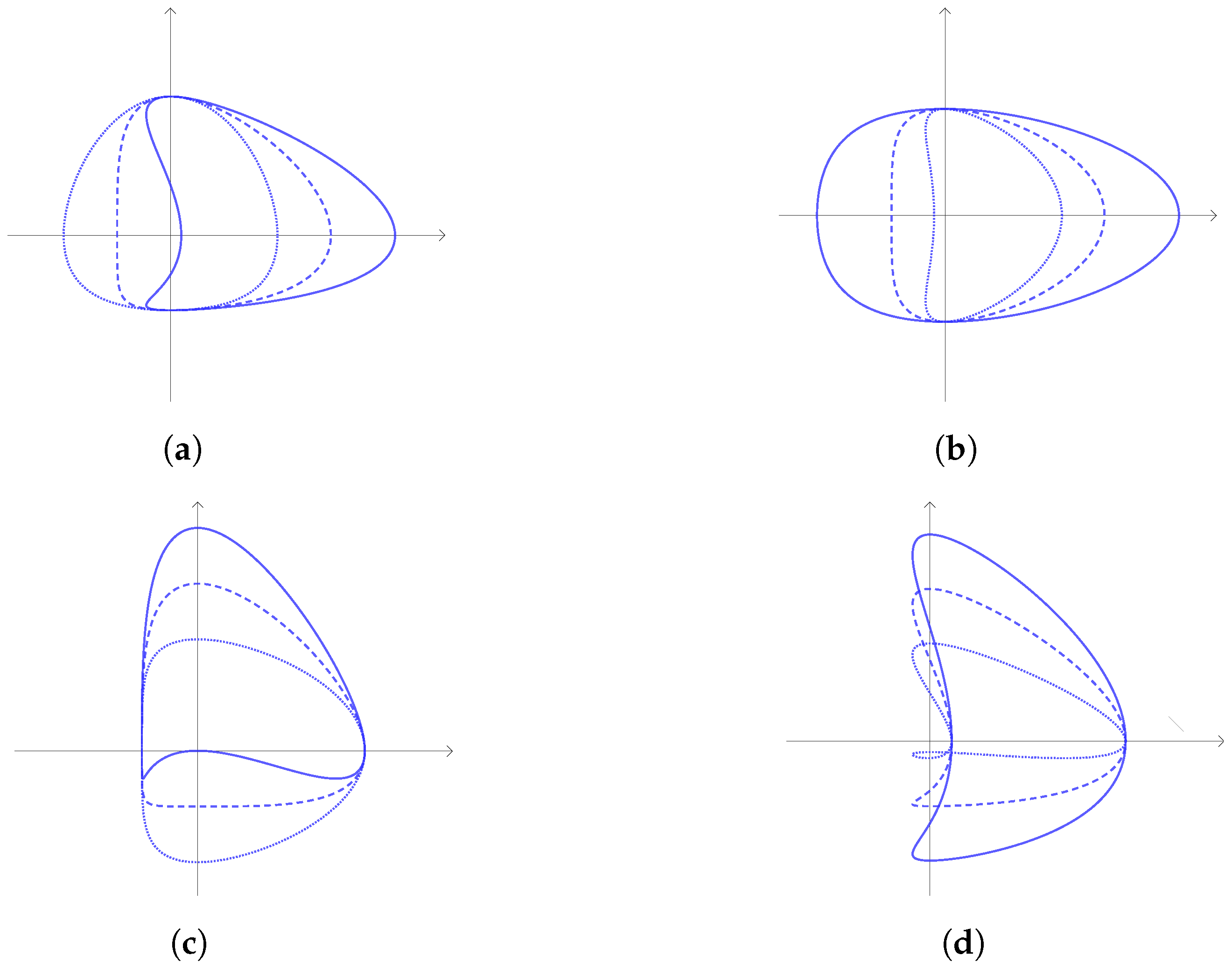
where sgn is the sign function. In Figure 2a, some superellipses with different choices of ϵ are shown. A superellipse can be deformed with the following transformations [59]:
  • Linear tapering along y axis
    { x = T a y y + 1 x y = y
    where 1 T 1 . The effect of this transformation is shown in Figure 2b.
  • Circular bending along the y axis
    { x = a y β y sin x a y β y y = a y β a y β y cos x a y β y
    where 1 β 1 , β 0 . The effect of this transformation is shown in Figure 2c.
  • Rotation and translation
    { x = x cos α y sin α + x 0 y = x sin α + y cos α + y 0
    where α [ 0 , 2 π [ , x 0 , y 0 R .
Figure 2. In each subfigure, a parameter changes and a x = a y = 1 . The dotted, dashed and solid curves correspond to the first, second and third value of the variable parameter, respectively. (a) ϵ = 0.7 ,   1 and 1.3 . (b) T = 0 ,   0.2 and 0.5 ( ϵ = 1 ). (c) β = 0.01 ,   0.6 and 0.8 ( ϵ = 1 ).
Symmetry 16 00755 g002
The model defined by composing Equations (1) and (3)–(5) is the deformed superellipse [12], and we used it as an object of comparison for the validation of our models. The proof of goodness was obtained by fitting all of our models to the 1227 prostate contours delineated by the radiologist. Moreover, the fitting performance was measured in terms of mean distance, Hausdorff distance and Dice similarity coefficient. The results show that our models are comparable to the deformed superellipse model from the point of view of error fitting. However, the main quality of our models is the simpler formulation; indeed, it can see in Section 2 that the models are defined by few and not complex equations. In addition, our models depend on a smaller number of parameters, and this implies a reduced cost in their implementation.
Other geometric descriptions of prostate shapes can be found in the literature. Saroul et al. [20] considered the model defined by only (1), (3) and (5). Tutar et al. [24] employed superquadrics, which are a 3D version of superellipses. Remaining in the 3D setting, prostate shape was modeled by Tutar [23] with spherical harmonics.
This paper is organized as follows. In Section 2, we present our models based on two parametric closed curves of the real plane (that we call CS and CC curves), and we study their main characteristics. In Section 3, we describe the validation process on our dataset of prostate shapes in the axial plane of MR images. The results of the validation are shown and discussed in Section 4 along with a comparison with the deformed superellipse model. Concluding remarks are in Section 5. Furthermore, in Appendix A, we report more mathematical studies of the curves, like special cases, elliptic Fourier descriptors, conditions for simple curves and area of the enclosed surfaces.

2. Our Models

To describe the contour of the prostate in the axial plane, we propose two types of curves as base models. We then formulate our general models considering any possible rotations and translations in the plane.
The first curve we present is defined in terms of parameters a , b , c , d R with b , d > 0 as follows:
{ x ( t ) = ( a cos ( t π ) + b ) cos ( t π ) y ( t ) = ( c sin ( t π ) + d ) sin ( t π ) 0 t 2 .
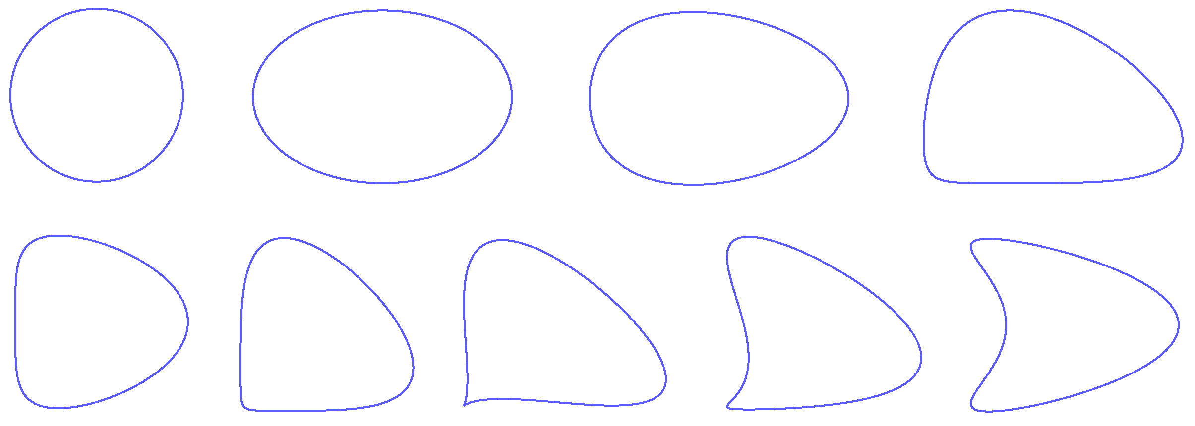
The parameters b and d are chosen to be positive because of symmetry reasons (see Section 2.2) and because for b = 0 or d = 0 , the curve is degenerate. In Figure 3, representative examples of simple curves as defined by (6) are provided. A curve is simple if it does not intersect itself (see also Appendix A.3); we show a picture of simple curves since they are the only cases of interest for the application we deal with in this paper. We named Equation (6) the CS curve (the term CS is an abbreviation to indicate the cosine function in the brackets of the expression of x and the sine function in the brackets of the expression of y).
The second curve is defined for a , b , c , d R and b , d 0 as follows:
{ x ( t ) = ( a cos ( t π ) + b ) cos ( t π ) y ( t ) = ( c cos ( t π ) + d ) sin ( t π ) 0 t 2 .
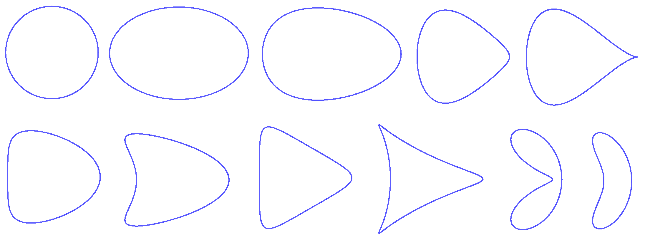
We are actually interested in the cases where none of the conditions a = b = 0 or b = c = 0 or c = d = 0 are satisfied, because each of them corresponds to a degenerate case. In Figure 4, representative examples of simple curves defined by (7) are depicted. With a meaning similar to the previous curve, we thus named Equation (7) the CC curve.
To the best of our knowledge, curves (6) and (7) have not been previously studied. Moreover, they include ellipses in the particular case a = c = 0 and other known curves, which are listed in Appendix A.1.
The models for prostate shapes which we propose in this paper are defined starting from (6) and (7) and considering any possible rotations and translations. The models are formulated more accurately in the following way:
{ x ˜ ( t ) = x ( t ) cos α y ( t ) sin α + x 0 y ˜ ( t ) = x ( t ) sin α + y ( t ) cos α + y 0 0 t 2 .
where α [ 0 , 2 π [ , x 0 , y 0 R and x ( t ) , y ( t ) are as in (6) or as in (7). These general models are then obtained by the rotation of angle α followed by a shift of x 0 along the x axis and a shift of y 0 along the y axis of a CS or a CC curve. They depend on seven parameters (a, b, c, d, α , x 0 , y 0 ). The value of α can be confined in the interval [ 0 , π [ since, as observed in Section 2.2, by changing the sign of the parameters a and b, one obtains the curve rotated by a straight angle around the origin.
In the next subsections, we describe various aspects of the two types of curves, dedicating a different paragraph to each one. Further analyses are reported in Appendix A.

2.1. Role of the Parameters

We start by discussing geometric meanings of the parameters a , b , c and d of the models. We refer to Figure 5, Figure 6 and Figure 7 for the considerations about CS curves and to Figure 8 and Figure 9 for the considerations about CC curves. The first observations we make are the following particular points of the curves determined by t = 0 , 1 2 , 1 and 3 2 .
CS curve:
x ( 0 ) = a + b y ( 0 ) = 0 , x ( 1 2 ) = 0 y ( 1 2 ) = c + d , x ( 1 ) = a b y ( 1 ) = 0 , x ( 3 2 ) = 0 y ( 3 2 ) = c d .
CC curve:
x ( 0 ) = a + b y ( 0 ) = 0 , x ( 1 2 ) = 0 y ( 1 2 ) = d , x ( 1 ) = a b y ( 1 ) = 0 , x ( 3 2 ) = 0 y ( 3 2 ) = d .
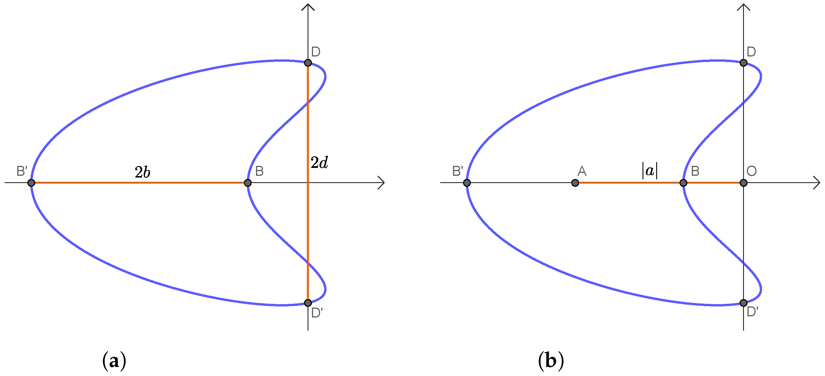
Taking into account (9) and (10), we can state that for every type of curve, b represents the half distance of the points determined by t = 0 and t = 1 (i.e., the points B and B in Figure 5 and Figure 8, respectively) and d represents the half distance of the points determined by t = 1 2 and t = 3 2 (i.e., the points D and D in Figure 5 and Figure 8, respectively). Hence, b and d play a role as indicators of thickness along the two axes, as it is also shown in Figure 6b,d and Figure 9b,d.
More rigorously, looking to (6) and (7), we note that if b increases, then x ( t ) for 0 t < 1 2 or for 3 2 < t 2 increases, and this means that the part of the curve from D to D (taken in an anticlockwise way) moves to the right if b increases. Conversely, x ( t ) for 1 2 < t < 3 2 decreases if b increases, and this means that the part of the curve from D to D (taken in an anticlockwise way) moves to the left if b increases. A similar argumentation can be applied to the parameter d. Concerning the parameters a and c, the geometric meanings vary between the two types of curves, so we make the related considerations separately below.

2.1.1. CS Curve

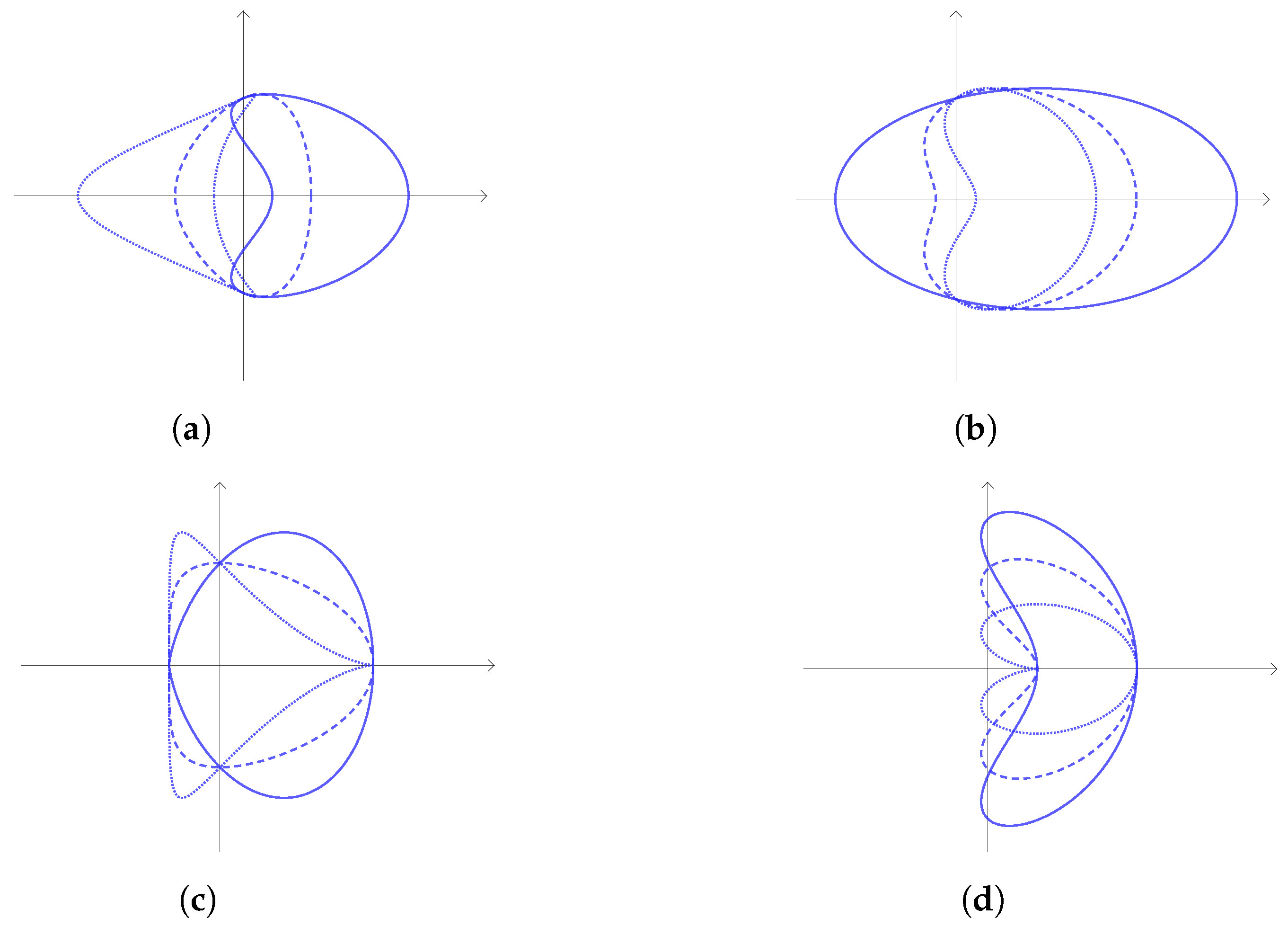
From Equation (9) we note that the middle point of the segment B B , labeled A in Figure 5, has an abscissa equal to a. This suggests that the parameter a regulates the stretching along the x axis (it can also be seen in Figure 6a). For the rigorous proof of the statement, we use Equation (6) and, in particular, that x ( t ) = a cos 2 ( t π ) + b cos ( t π ) : for a fixed 0 t 2 except for t = 1 2 and t = 3 2 , if a increases, then x ( t ) increases too. This means that if a increases, the curve stretches to the right of the plane.
A similar observation can be made for the parameter c. The middle point of the segment D D , labeled C in Figure 5b, has an ordinate equal to c, and furthermore, the parameter c regulates the stretching along the y axis, as shown in Figure 6c.
Figure 5. Geometric meaning of the parameters a ,   b ,   c and d of a CS curve. B ( a + b   , 0 ) and B ( a b ,   0 ) are the points determined by t = 0 and t = 1 , respectively; D ( 0 ,   c + d ) and D ( 0 ,   c d ) are the points determined by t = 1 2 and t = 3 2 , respectively; A ( a ,   0 ) is the middle point of the segment B B ; C ( 0 ,   c ) is the middle point of the segment D D . (a) The length of the segment B B is 2 b . The length of the segment D D is 2 d . (b) The length of the segment O A is | a | . The length of the segment O C is | c | .
Symmetry 16 00755 g005
Figure 6. Some examples of CS curves. In each subfigure, three parameters are fixed and the remaining one changes. The dotted, dashed and solid curves correspond to the first, second and third value of the variable parameter, respectively. (a) Fixed parameters: b = 1 , c = 0.3 , d = 1 . Variable parameter: a = 0 ,   0.5 and 1.1 . (b) Fixed parameters: a = 0.5 , c = 0 , d = 1 . Variable parameter: b = 0.6 ,   1 and 2. (c) Fixed parameters: a = 0.5 , b = 1 , d = 1 . Variable parameter: c = 0 ,   0.5 and 1. (d) Fixed parameters: a = 1 , b = 0.8 , c = 0.4 . Variable parameter: d = 0.5 ,   1 and 1.5 .
Symmetry 16 00755 g006
Other parameters of particular interest are a b and c d . The first value indicates if the curve has a concavity (like in Figure 7a,d) or a ‘flat side’ on the right/left part (like in Figure 7b), while the second value specifies the presence of a concavity (like in Figure 7c) or a ‘flat side’ on the top/bottom part. More precisely, see the following:
  • The curve has a concavity around B if and only if a b < 1 2 ;
  • The curve has a ‘flat side’ around B if and only if a b = 1 2 ;
  • The curve has a ‘flat side’ around B if and only if a b = 1 2 ;
  • The curve has a concavity around B if and only if a b > 1 2 ;
  • The curve has a concavity around D if and only if c d < 1 2 ;
  • The curve has a ‘flat side’ around D if and only if c d = 1 2 ;
  • The curve has a ‘flat side’ around D if and only if c d = 1 2 ;
  • The curve has a concavity around D if and only if c d > 1 2 .
Furthermore, the concavity is more accentuated for greater values of | a b | (respectively, | c d | ). The statements above can be proved by studying the signed curvature k ( t ) = x ( t ) y ( t ) x ( t ) y ( t ) ( x ( t ) 2 + y ( t ) 2 ) 3 2 for t = 0 , 1 2 , 1 , 3 2 [60]. For instance, k ( 0 ) = 2 a + b d 2 , so k ( 0 ) < 0 , i.e., there is a concavity around B if a b < 1 2 .
Figure 7. Some examples of CS curves with the values of the indicators a b and c d of concavity. (a) a b = 1.2 and c d = 0.3 . (b) a b = 0.5 and c d = 0 . (c) a b = 0.3 and c d = 2 . (d) a b = 0.7 and c d = 0.7 .
Symmetry 16 00755 g007

2.1.2. CC Curve

For the parameter a, we can make the same remarks for the previous curve, i.e., a is the abscissa of the middle point of the segment B B , and moreover, it regulates the stretching along the x axis. The reference figures are Figure 8 and Figure 9a.
The parameter c plays a different role in the case of CS curves. To visualize the effect of this parameter on the curve, we refer to Figure 8 for the points and to Figure 9c. Increasing the value of c, the part of the curve from B to D moves up, the part of the curve from D to B moves down, the part of the curve from B to D moves up and the part of the curve from D to B moves down (each part is taken in an anticlockwise way from the first to the second point excluding the two points).
To prove this statement, we use (7): for example, the part of the curve from B to D (excluding these two points) corresponds to the values of t from 0 and 1 2 ; therefore, cos ( t π ) > 0 and sin ( t π ) > 0 . Thus, for a fixed 0 < t < 1 2 , we have cos ( t π ) sin ( t π ) > 0 , so if c increases, then y ( t ) increases. For the other parts of the curve, the cos ( t π ) and sin ( t π ) may have a different sign, so the argument must be consequently modified.
Moreover, as for CS curves, the parameter a b is an indicator of concavity:
  • The curve has a concavity around B if and only if a b < 1 2 ;
  • The curve has a ‘flat side’ around B if and only if a b = 1 2 ;
  • The curve has a ‘flat side’ around B if and only if a b = 1 2 ;
  • The curve has a concavity around B if and only if a b > 1 2 .
Figure 8. Geometric meaning of the parameters a ,   b and d of a CC curve. B ( a + b ,   0 ) and B ( a b ,   0 ) are the points determined by t = 0 and t = 1 , respectively; D ( 0 ,   d ) and D ( 0 ,   d ) are the points determined by t = 1 2 and t = 3 2 , respectively; A ( a ,   0 ) is the middle point of the segment B B . (a) The length of the segment B B is 2 b . The length of the segment D D is 2 d . (b) The length of the segment O A is | a | .
Symmetry 16 00755 g008
Figure 9. Some examples of CC curves. In each subfigure, three parameters are fixed and the remaining one changes. The dotted, dashed and solid curves correspond to the first, second and third value of the variable parameter, respectively. (a) Fixed parameters: b = 0.7 , c = 0.3 , d = 1 . Variable parameter: a = 1 ,   0 and 1. (b) Fixed parameters: a = 0.8 , c = 0.5 , d = 1 . Variable parameter: b = 0.6 ,   1 and 2. (c) Fixed parameters: a = 0.5 , b = 1 , d = 1 . Variable parameter: c = 1 ,   0 and 1. (d) Fixed parameters: a = 1 , b = 0.5 , c = 0.5 . Variable parameter: d = 0.5 ,   1 and 1.5 .
Symmetry 16 00755 g009

2.2. Symmetries and Invariants

Here we discuss the actions of some transformations on the parameters and general symmetries of the curves. Parts of the transformations constitute invariants, which can limit the variability of some parameters. The statements below can be easily proved directly from the expressions (6) and (7) and taking into account basic properties of the sine and cosine functions.

2.2.1. CS Curve

  • The transformation a a gives the symmetric curve with respect to the y axis. Thus, if a = 0 , the curve is symmetric with respect to the y axis.
  • The transformation c c gives the symmetric curve with respect to the x axis. Thus, if c = 0 , the curve is symmetric with respect to the x axis.
  • Each one of the transformations b b and d d leaves the curve invariant. This reason, together with the degenerate cases b = 0 or d = 0 , justifies our choice to consider b and d as positive numbers made in (6).
  • The transformation ( a , c ) ( a , c ) gives the symmetric curve with respect to the origin (or, equivalently, the curve rotated by a straight angle with its center as the origin).
  • The transformation ( a , b , c , d ) ( c , d , a , b ) gives the symmetric curve with respect to the line y = x . Thus, if a = c and b = d , the curve is symmetric with respect to the line y = x .

2.2.2. CC Curve

  • The curve is always symmetric with respect to the x axis.
  • Each one of the transformations ( a , b ) ( a , b ) , ( a , c ) ( a , c ) and ( a , d ) ( a , d ) gives the symmetric curve with respect to the y axis (or, equivalently, the curve rotated by a straight angle with its center at the origin, as in the previous remark).
  • Each one of the transformations ( b , c ) ( b , c ) , ( b , d ) ( b , d ) and ( c , d ) ( c , d ) leaves the curve invariant. For this reason, we assume that b and d are non-negative numbers in (6).

3. Validation of the Models

This section is devoted to the assessment of the models for the representation of prostate shape in the axial plane of MR images. Thanks to the results we obtained (see Section 4), we believe that these models may be useful in specific fields of image analysis (such as segmentation, classification, recognition).
Our dataset is made of 1227 slices of prostate MR images coming from a total of 50 patients. The slices have a resolution of 672 × 672 and a pixel size of 0.27 mm × 0.27 mm, and the distance between two consecutive slices is 2.5 mm. Figure 10 shows an example of an MR image on the left, a cropped and enlarged version of it in the center and the prostate contour (ground truth) delineated by the radiologist on the right.
As one can see, the prostate contours in Figure 1 are very similar, with eventual rotations, to the examples of model curves in Figure 3 and Figure 4. Of course, visual correspondence is not sufficient to check if a model well represents an object. Therefore, we proceeded to a numerical validation of the model (8). We point out that here we only take care of the validation of the models. Future works will be oriented to their service in a segmentation process.
The validation consisted of three parts: the extraction of the prostate contours in MR images made by a radiologist with more than 10 years of experience, the model fitting and its performance valuation.
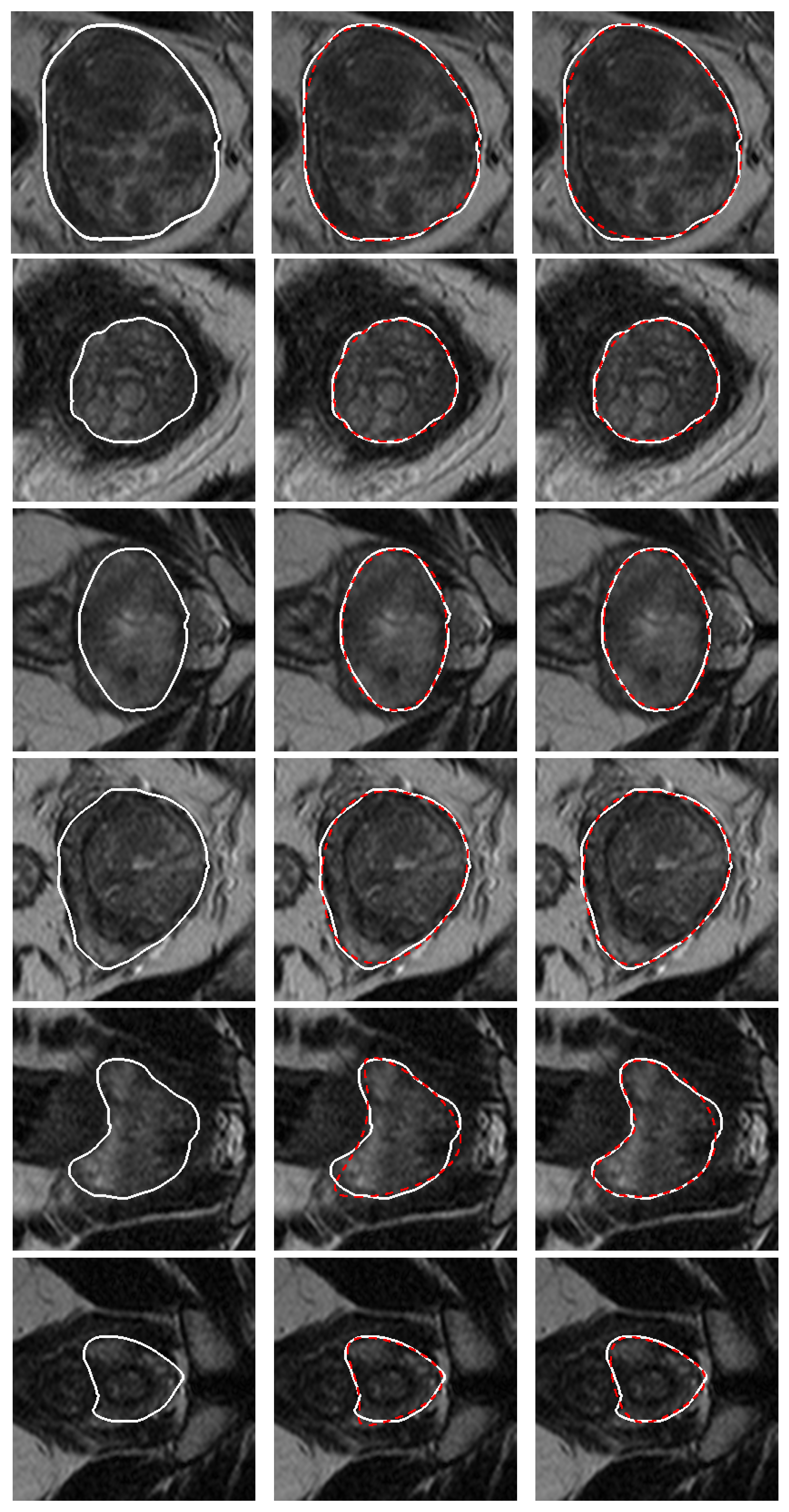
First of all, the expert manually extracted the prostate contours in each of the 1227 slice images in our database. Then, the model (8) was validated on the ground truths one time for each of curves (6) and (7). In other words, following the method described below, we found the best CS and CC curves that approximate the given contour. Finally, we selected the best one of the two results for the given contour. Figure 11 shows some ground truths and the relative fittings with CS and CC curves.
In detail, the approximation process was set as follows. We denote by C p a prostate contour as a set of points ( x ˜ , y ˜ ) in a 2D digital image and by C m = C m ( a , b , c , d , α , x 0 , y 0 ) the model curve given by (8) (and (6) or (7), depending on the type of curve). For a given contour C p and each of the two types of curve (CS and CC), we searched the parameters a , b , c , d , α , x 0 , y 0 of the model C m = C m ( a , b , c , d , α , x 0 , y 0 ) to find which best fits the prostate contour, in the sense that it minimizes the following metric:
d m ( C p , C m ( a , b , c , d , α , x 0 , y 0 ) ) = mean ( x ˜ , y ˜ ) C p min t [ 0 , 2 ] d ( ( x ˜ , y ˜ ) , ( x ( t ) , y ( t ) ) )
that is, the mean distance between the generic point of C p and the closest point of the model C m ( a , b , c , d , α , x 0 , y 0 ) [12]. To further evaluate the fitting of the curve found by the minimization above, we also considered the Hausdorff distance [12,61] and the Dice similarity coefficient [62,63]. The Hausdorff distance
d H ( C p , C m ( a , b , c , d , α , x 0 , y 0 ) ) = max ( x ˜ , y ˜ ) C p min t [ 0 , 2 ] d ( ( x ˜ , y ˜ ) , ( x ( t ) , y ( t ) ) )
is the maximum distance between the generic point of C p and the closest point of the model C m ( a , b , c , d , α , x 0 , y 0 ) . The Dice similarity coefficient is
D S C = 2 | S p S m | | S p | + | S m | ,
where | · | denotes the area of a surface, S p is the prostate surface (i.e., the surface enclosed by the contour C p ) and S m is the surface enclosed by the curve C m .
The local minima for (11) were searched using the gradient descent method, iterating the process until the variation in (11) becomes negligible. In the procedure, all the curves were discretized, with 160 points individuated by uniformly distributed points { t i } in the interval [ 0 , 2 ] . The initialization of the process set the ellipse with axes of axial sizes l x and l y of the prostate contour and centered in the center of the prostate (see Figure 12a). In particular, this corresponds to the following parameters: a = c = 0 , b = l x 2 and d = l y 2 . When the prostate has a concavity and the process starts with this ellipse, the gradient descent method may find a local minimum which does not give a perfect approximation (for example, this is the case in Figure 12b). For a better result, the method was repeated, and the initial curve taken was one with a concavity if the mean distance was higher than a fixed value at the end of the process (see Figure 12c). This way, a better fitting was usually found, as shown in Figure 12d. More precisely, for the second initialization, we set a = b = l x 2 , c = 0 and d = l y 2 for both the CC and the CS fitting.
Finally, we compared our models with the deformed superellipse model employed in [12], which we described in the Introduction. In particular, to fit the deformed superellipse model to the prostate contours, we followed an approach similar to the one explained for our models. Namely, employing the gradient descent method, for each of the 1227 ground truths, we searched the parameters a x , a y , ϵ , T, β , α , x 0 , y 0 of the deformed superellipse that best fit the given contour, i.e., that minimized the mean distance (11). The base curve (1) was implemented by (2) taking, as before, 160 points { t i } uniformly distributed in the interval [ 0 , 2 ] . Then the transformations (3)–(5) were applied. The initial choice of parameters was set corresponding to the initial curve in our models’ validation.

4. Results and Discussion

The results of the validation are reported in Table 1, where in each entry, the first and the second numbers represent the mean and the standard deviation of the corresponding metric over all the 1227 contours, respectively. Table 2 shows the time employed (on an Intel Core i5-9500 CPU running at 3 GHz) for fitting a given contour.
In the first row are the performance metrics when the best model between CS and CC is selected for a given contour. The model selected is the one that gives the lowest mean distance value (11). In Figure 13, two ground truths with the fittings of each model are shown. In particular, we chose two contour examples in which a different model provides the best approximation.
The performance of a single model (CS or CC) is detailed in the second and third rows of Table 1. Finally, the performance metrics of the deformed superellipse model are reported in the last row of Table 1.
The performance metrics of our models are comparable to ones of the deformed superellipse model (a slightly better result is obtained when the best curve between CS and CC is selected as the model). However, concerning the time employed for the fitting process, there is a significant difference. Finding a deformed superellipse that best fits a contour requires about 15 times the cost necessary for fitting a CS or CC model curve.
Furthermore, the deformed superellipse model depends on eight parameters ( a x , a y , ϵ , T, β , α , x 0 and y 0 ); in contrast, each of our models (CS or CC) (8) depends on seven parameters (a, b, c, d, α , x 0 and y 0 ). Hence, this represents an important benefit of our models because it provides a more straightforward definition and it is also the reason for the reduced computational cost in the fitting. Indeed, to obtain a more precise fitting of deformed superellipses, the method was repeated for different fixed values of b, and this caused a greater time of execution. Moreover, CS and CC curves have a detailed description in Section 2 and in Appendix A. This could help to make specific and quantitative analyses of the prostate shape.
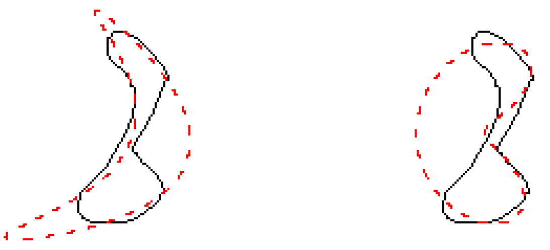
As a limitation, we remark that in some, but few, cases, the prostate has an atypical contour, different to the ones represented in Figure 1, which is not well approximated by the CS and CC curves. One of these outlier cases is shown in Figure 14 with its fittings.
Our goal in this paper was to present and validate two models for prostate shape. Due to the assessment of our models, we believe they can be adopted in prostate segmentation processes. A possible scheme for an automatic segmentation may be the following. A first and approximative prostate contour is searched with elementary image analysis techniques like texture evaluations or morphological operators or with more sophisticated methods like machine/deep learning [28]. Then the CS and CC models are fitted to the first contour to reproduce a more real shape. Alternatively, a second approach may be the definition of an active contour [64] whose shape is restricted to CS and CC curves.

5. Conclusions

We proposed two geometric 2D models for prostate shape in MR images. Each model is defined starting from a parametric curve and depends on a total of seven parameters. We described the parametric curves and validated the models on a database of prostate contours (ground truths) extracted by a radiologist. As part of the validation, we also compared to the deformed superellipse model employed for prostate segmentation in TRUS images in [12]. The results show that our models are comparable with the deformed superellipse model in terms of distance and overlapping errors. We highlight values for the mean distance equal to 0.56 ± 0.32 mm and 0.61 ± 0.32 mm and DSC values equal to 96.7 % ± 3.1 % and 96.5 % ± 2.7 % for the best of our models and the deformed superellipse model, respectively. However, our models have a more compact mathematical expression, depend on fewer parameters and require less time for contour fitting.

Author Contributions

Conceptualization, R.C.; methodology, R.C. and D.T.; software, R.C.; validation, R.C.; formal analysis, R.C.; investigation, R.C.; resources, A.C., G.S. and D.T.; data curation, A.C. and G.S.; writing—original draft preparation, R.C.; writing—review and editing, R.C., A.C., G.S. and D.T.; visualization, R.C.; supervision, A.C. and D.T.; project administration, A.C. and D.T.; funding acquisition, R.C. and D.T. All authors have read and agreed to the published version of the manuscript.

Funding

R.C. acknowledges partial financial supports by the European Union through the Italian Ministry of University and Research (FSE - REACT EU, PON Ricerca e Innovazione 2014-2020, CUP B75F21002310001), by the Università degli Studi di Palermo (FFR2024 “Corso”) and by the “Gruppo Nazionale per l’Analisi Matematica, la Probabilità e le loro Applicazioni” (GNAMPA—INdAM) (CUP E53C23001670001). The research leading to these results was also supported by the European Union- NextGenerationEU through the Italian Ministry of University and Research under PNRR–M4C2–I1.3 Project PE_00000019 “HEAL ITALIA” to D.T. (CUP B73C22001250006).

Institutional Review Board Statement

This study is a retrospective study and written informed consent was waived by the ethical committee of our hospital. All the patients who underwent MRI examination provided written informed consent for the use of their anonymized MRI studies for research purposes.

Informed Consent Statement

Informed consent was obtained from all subjects involved in the study.

Data Availability Statement

The datasets presented in this article are not readily available.

Conflicts of Interest

The authors declare no conflicts of interest.

Appendix A. Further Analysis of CS and CC Curves

In Section 2, we gave geometric meanings to the parameters and studied symmetries and invariants. In addition, we investigated the curves (6) and (7) also under other aspects (special cases, elliptic Fourier descriptors, conditions for the curves to be simple and formulas for the enclosed area), and we collected the results in this Appendix. We also remark that the curves (6) and (7) are, in particular, algebraic curves with degrees equal to four or lower in some cases. The implicit (Cartesian form) equations, which are omitted for their complicated expressions, can be obtained by eliminating the sine and cosine functions in (6) and (7) or by Sylvester’s matrix elimination method [65] (see also [66]).

Appendix A.1. Special Cases

For some particular values of the parameters, we can recover some known curves [67].

Appendix A.1.1. CS Curve

  • For a = c = 0 and b = d = r , the curve is the circle centered in the origin with radius r.
  • For a = c = 0 , the curve is the ellipse centered in the origin with semiaxes b and d.

Appendix A.1.2. CC Curve

  • For a = c = 0 and b = d = r , the curve is the circle centered in the origin with radius r.
  • For a = c = 0 , the curve is the ellipse centered in the origin with semiaxes b and d.
  • For a = d = 0 , the curve is a Lissajous curve.
  • For a = d = 0 and b = c = 1 , the curve is the lemniscate of Gerono.
  • For a = b = c = d , the curve is a cardioid.
  • For a = c and b = d , the curve is a limaçon.
  • For a = c = 2 b = 2 d , the curve is a limaçon trisectrix.
  • For a = 0 and c = d , the curve is a translation of a piriform quartic.
  • For a = b = c = d , the curve is a translation of a deltoid.
  • For a = c and b = d , the curve is a translation of a hypotrochoid.
  • For a = 1 , b = 1 2 , c = 1 and d = 1 2 , the curve is a translation of a regular trifolium.

Appendix A.2. Elliptic Fourier Descriptors

Taking into account the formulas cos 2 ( t π ) = 1 + cos ( 2 t π ) 2 , sin 2 ( t π ) = 1 cos ( 2 t π ) 2 and sin ( t π ) cos ( t π ) = 1 2 sin ( 2 t π ) , the curves have the following Fourier basis representations [68,69] with a number of harmonics equal to 2.

Appendix A.2.1. CS Curve

x ( t ) y ( t ) = a 2 c 2 + b 0 0 d cos ( t π ) sin ( t π ) + a 2 0 c 2 0 cos ( 2 t π ) sin ( 2 t π )

Appendix A.2.2. CC Curve

x ( t ) y ( t ) = a 2 0 + b 0 0 d cos ( t π ) sin ( t π ) + a 2 0 0 c 2 cos ( 2 t π ) sin ( 2 t π )

Appendix A.3. Simple Curves

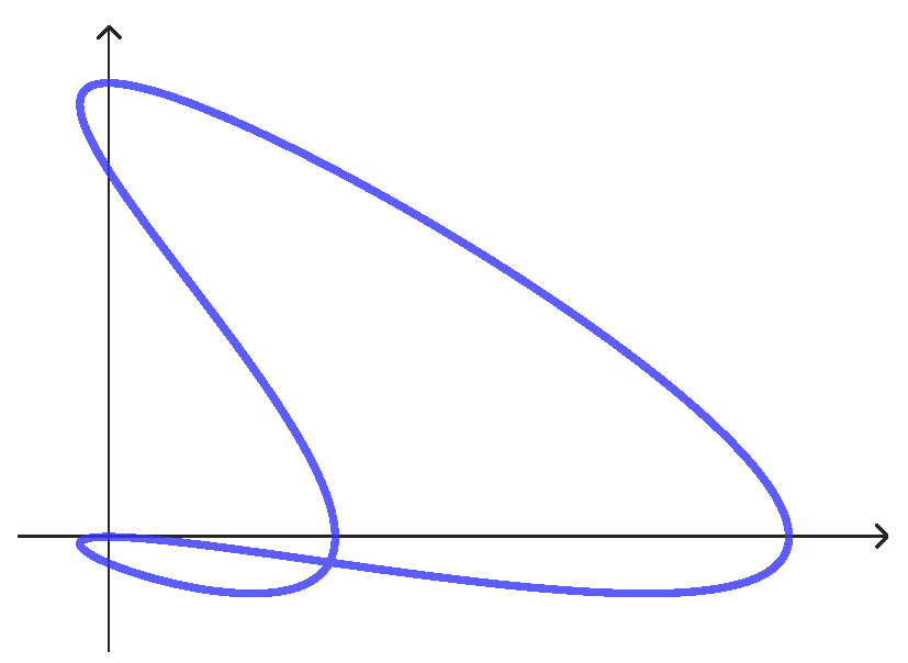
For some choices of parameters, the curves turn out to be nonsimple, i.e., each intersects itself (see as an example Figure A1). A nonsimple curve is characterized by the existence of 0 t 1 , t 2 < 2 such that t 1 t 2 and x ( t 1 ) = x ( t 2 ) and y ( t 1 ) = y ( t 2 ) (the value t = 2 is not taken into consideration because of the periodicity of the sine and cosine functions). In relation to the application that we discussed in Section 4, it is interesting to have necessary and sufficient conditions on the parameters in order for the curves to be simple. We give the conditions, along with their proofs, for each type of curve below.
Figure A1. A nonsimple CS curve. The parameters are a = 2 , b = 1 , c = 1 , d = 1 .
Symmetry 16 00755 g0a1

Appendix A.3.1. CS Curve

Theorem A1. 
Let b , d > 0 . The CS curve (6) is simple if and only if
a 2 d 2 + b 2 c 2 4 a 2 c 2 .
Proof. 
First, we assume that (A1) holds and prove that the curve is simple. So let t 1 , t 2 [ 0 , 2 [ with t 1 t 2 such that x ( t 1 ) = x ( t 2 ) and y ( t 1 ) = y ( t 2 ) , i.e.,
( a cos ( t 1 π ) + b ) cos ( t 1 π ) = ( a cos ( t 2 π ) + b ) cos ( t 2 π ) ( c sin ( t 1 π ) + d ) sin ( t 1 π ) = ( c sin ( t 2 π ) + d ) sin ( t 2 π ) .
The equations yield
( cos ( t 1 π ) cos ( t 2 π ) ) ( a ( cos ( t 1 π ) + cos ( t 2 π ) ) + b ) = 0 ( sin ( t 1 π ) sin ( t 2 π ) ) ( c ( sin ( t 1 π ) + sin ( t 2 π ) ) + d ) = 0 .
Therefore, since t 1 t 2 , we have
a ( cos ( t 1 π ) + cos ( t 2 π ) ) = b c ( sin ( t 1 π ) + sin ( t 2 π ) ) = d .
Clearly, (A3) has no solution if a = 0 or c = 0 . So, in the following, we assume that a , c 0 and rewrite (A3) as
sin ( t 1 + t 2 2 π ) sin ( t 1 t 2 2 π ) = b 2 a cos ( t 1 + t 2 2 π ) sin ( t 1 t 2 2 π ) = d 2 c ,
which implies that
sin 2 t 1 t 2 2 π = b 2 4 a 2 + d 2 4 c 2 .
We now analyze three cases:
  • If a 2 d 2 + b 2 c 2 > 4 a 2 c 2 holds, Equation (A5), and then the system (A2) has no solutions, i.e., the curve is simple.
  • If a 2 d 2 + b 2 c 2 = 4 a 2 c 2 holds, Equation (A5) means sin ( t 1 t 2 2 π ) = ± 1 . Interchanging, eventually, t 1 with t 2 , we can suppose that sin ( t 1 t 2 2 π ) = 1 , and then, taking into account that t 1 , t 2 [ 0 , 2 [ , we have t 1 t 2 = 1 . We write s : = t 1 + t 2 . So we have that t 1 = s + 1 2 and t 2 = s 1 2 . Imposing that t 1 , t 2 [ 0 , 2 [ , we find that
    s [ 1 , 3 [ [ 1 , 5 [ = [ 1 , 3 [ .
    For symmetry reasons (see Section 2.2), we can confine ourselves to the case a > 0 and c < 0 ; therefore, by (A4), s ] 0 , 1 [ , which is in contradiction to (A6).
    To summarize, in the case a 2 d 2 + b 2 c 2 = 4 a 2 c 2 , the system (A2) has no solutions, i.e., the curve is simple.
Now we assume that (A1) does not hold, i.e., a 2 d 2 + b 2 c 2 < 4 a 2 c 2 , and prove that the curve is not simple. Hence, there exist r ] 0 , 1 [ such that sin ( r π ) = b 2 4 a 2 + d 2 4 c 2 and s ] 0 , 2 [ such that
sin ( s π ) = b 2 a b 2 4 a 2 + d 2 4 c 2 cos ( s π ) = d 2 c b 2 4 a 2 + d 2 4 c 2 .
Let t 1 = r + s + 2 m and t 2 = s r + 2 n with m , n Z chosen in such a way so that t 1 , t 2 [ 0 , 2 [ . In particular, we have t 1 t 2 because r cannot be an integer. We have that t 1 t 2 2 = r + m n and t 1 + t 2 2 = s + m + n , so (A4) and (A5) are satisfied. This means that (A2) is satisfied and the proof is completed.  □

Appendix A.3.2. CC Curve

We assume that not one of the conditions a = b = 0 or b = c = 0 or c = d = 0 holds since these are the cases of a degenerate curve.
Theorem A2. 
Let us assume that b , d 0 and that not one of the conditions a = b = 0 or b = c = 0 or c = d = 0 holds. The CC curve (7) is simple if and only if one of the following conditions is satisfied:
(i) 
c = 0 ;
(ii) 
a = 0 and d | c | ;
(iii) 
a , b , c 0 , d | c | and b 2 a b a d c 0 ;
(iv) 
a , b , c 0 , d | c | and b 2 a b a d c 1 ;
(v) 
a , b , c 0 , d | c | , 0 < b 2 a b a d c < 1 and b 2 | a | b a d c .
Proof. 
The proof is divided into two parts: in the first part, we assume that one of the statements ((i)–(v)) is satisfied and prove that the curve is simple. Let t 1 , t 2 [ 0 , 2 [ with t 1 t 2 such that x ( t 1 ) = x ( t 2 ) and y ( t 1 ) = y ( t 2 ) , i.e.,
( a cos ( t 1 π ) + b ) cos ( t 1 π ) = ( a cos ( t 2 π ) + b ) cos ( t 2 π ) ( c cos ( t 1 π ) + d ) sin ( t 1 π ) = ( c cos ( t 2 π ) + d ) sin ( t 2 π ) .
The equations can be rewritten as
( cos ( t 1 π ) cos ( t 2 π ) ) ( a ( cos ( t 1 π ) + cos ( t 2 π ) ) + b ) = 0 ( c cos ( t 1 π ) + d ) sin ( t 1 π ) = ( c cos ( t 2 π ) + d ) sin ( t 2 π ) .
We now analyze the different cases.
Case (i). If c = 0 , then d 0 ; so by the second line of (A8) and the fact that t 1 t 2 , we have cos ( t 1 π ) = cos ( t 2 π ) . Assuming that the latter condition is true, then 2 b cos ( t 1 π ) = 0 for the first line of (A8), which gives that t 1 = 1 2 = t 2 or t 1 = 3 2 = t 2 since we can exclude that b = 0 . Hence, the curve is simple.
Case (ii). If a = 0 and d | c | , then b 0 and the first line of (A8), together with t 2 t 1 , implies that t 2 = 2 t 1 . Assuming that the latter condition is true, we have that ( c cos ( t 1 π ) + d ) sin ( t 1 π ) = 0 by the second line of (A7). So we can say sin ( t 1 π ) = 0 or c cos ( t 1 π ) + d = 0 . Taking into account that t 1 , t 2 [ 0 , 2 [ , if sin ( t 1 π ) = 0 then t 1 = t 2 , which is not allowed. On the other hand, the equation
c cos ( t 1 π ) + d = 0 .
has no solutions if d > | c | . If c 0 and d = c , Equation (A9) has solution t 1 = 1 , so t 2 = 1 = t 1 , which contradicts the assumption of t 1 and t 2 . If c 0 and d = c , Equation (A9) has solutions t 1 = 0 and t 2 = 2 t 1 = 2 [ 0 , 2 [ . We conclude that the curve is simple.
Before we move on to cases (iii)–(v), we make some observations. Since all the cases impose d | c | , for the considerations we have made about (A9), we can exclude that cos ( t 1 π ) cos ( t 2 π ) = 0 . So, by the first line of (A8), we can assume that
a ( cos ( t 1 π ) + cos ( t 2 π ) ) + b = 0 ,
which we will be able to be rewritten as
cos t 1 + t 2 2 π cos t 1 t 2 2 π = b 2 a
because we assume that a 0 . On the other hand, the second equation in (A7) is equivalent to
d ( sin ( t 1 π ) sin ( t 2 π ) ) = c 2 ( sin ( 2 t 2 π ) sin ( 2 t 1 π ) )
and also to
d cos t 1 + t 2 2 π sin t 1 t 2 2 π = c 2 cos ( t 1 + t 2 ) π sin ( t 2 t 1 ) π = c cos ( t 1 + t 2 ) π sin t 1 t 2 2 π cos t 1 t 2 2 π .
Since sin t 1 t 2 2 π 0 , because t 1 t 2 , we derive that
d cos t 1 + t 2 2 π = c cos ( t 1 + t 2 ) π cos t 1 t 2 2 π = c 2 cos 2 t 1 + t 2 2 π 1 cos t 1 t 2 2 π .
Multiplying by cos t 1 t 2 2 π in (A13), we obtain
d cos t 1 + t 2 2 π cos t 1 t 2 2 π = c cos ( t 1 + t 2 ) π cos t 1 t 2 2 π = c 2 cos 2 t 1 + t 2 2 π 1 cos 2 t 1 t 2 2 π .
By (A11), the previous equation becomes
b d 2 a = b 2 c 2 a 2 + c cos 2 t 1 t 2 2 π ,
and since c 0 is assumed, it is equivalent to
cos 2 t 1 t 2 2 π = b 2 2 a 2 b d 2 a c = b 2 a b a d c .
We now continue to examine the cases in the statement.
Cases (iii)–(iv). Let a , b , c 0 . Equation (A14) has no solutions if
b 2 a b a d c < 0 or b 2 a b a d c > 1 .
If b 2 a b a d c = 0 , then there are no solutions by (A14) and (A11). If b 2 a b a d c = 1 , then by (A14), we have that t 1 t 2 is an even number, but this cannot be true if t 1 , t 2 [ 0 , 2 [ . In conclusion, (A13) cannot be realized, i.e., the curve is simple.
Case (v). Let a , b , c 0 , d | c | , 0 < b 2 a b a d c < 1 . By (A11) and (A14), we have
cos 2 t 1 + t 2 2 π = b 2 a b a d c .
If b 2 | a | > b a d c , then (A15) has no solutions. If b 2 | a | = b a d c , then t 1 + t 2 is an even number by (A15); taking into account that t 1 + t 2 [ 0 , 4 [ , we necessarily have t 1 + t 2 = 0 , meaning that t 1 = t 2 = 0 , which is not allowed by the assumption, or t 1 + t 2 = 2 , which implies the contradiction that b = 0 by (A10). In conclusion, the curve is simple.
We now prove that the curve is not simple if not one of the statements (i–v) is satisfied; in other words, we assume that one the following statements holds:
  • c 0 , d < | c | ;
  • a , c 0 , 0 < b 2 a ( b a d c ) < 1 and b 2 | a | < b a d c ;
  • b = 0 .
If 1. holds, then there exists t 1 ] 0 , 2 [ such that c cos ( t 1 π ) + d = 0 and t 1 1 . Thus, the pair ( t 1 , t 2 ) with t 2 = 1 t 1 is a solution of (A8), i.e., x ( t 1 ) = x ( t 2 ) and y ( t 1 ) = y ( t 2 ) . Since t 1 1 , we have that t 1 t 2 ; hence, the curve is not simple.
If 2. holds, then there exist r , s [ 0 , 2 [ such that
cos r π = b 2 a b a d c , cos s π = b 2 a b 2 a b a d c .
Let t 1 = r + s + 2 m and t 2 = s r + 2 n with m , n Z chosen in such a way so that t 1 , t 2 [ 0 , 2 [ . We have that t 1 t 2 2 = r + m n and t 1 + t 2 2 = s + m + n , so (A11) and (A12) are satisfied, i.e., (A7) holds. Taking into account that t 1 t 2 because r cannot be an integer, the curve is not simple.
If 3. holds, then ( t 1 , t 2 ) = ( 0 , 1 ) is a solution of (A7), so the curve is not simple.  □
Note that by Theorem A2, if a CC curve is simple then b , d 0 .
Figure A2. Some examples of nonsimple CC curves. (a) a = 1 , b = 0.5 , c = 1.5 , d = 1 . (b) a = 0.5 , b = 1.5 , c = 1.5 , d = 1 . (c) a = 1 , b = 0 , c = 1 , d = 1 . (d) a = 1.5 , b = 1 , c = 1 , d = 1 . (e) a = 1.5 , b = 1 , c = 1.5 , d = 1 .
Symmetry 16 00755 g0a2

Appendix A.4. Area of the Enclosed Surface

Under the condition of a simple curve, a unique surface enclosed by the curve is formed. Note that with the assumption about b and d that we made in the Introduction, the curves (6) and (7) are positively orientated, i.e., in the anticlockwise way. The area of the surface enclosed by the curve is as follows:
  • A = π b d for CS curves (so it does not depend on the parameters a , c and it is the same as the area of the surface inside an ellipse with semiaxes b and d);
  • A = π a c 2 + b d for CC curves.
The area of the surface can be calculated by the Gauss–Green formulas. Here we give, as an example, the proof of the formula for simple CS curves. By (6) and the Gauss–Green formula,
A = 0 2 y ( t ) x ( t ) d t = π 0 2 ( c sin ( t π ) + d ) sin ( t π ) ( 2 a cos ( t π ) + b ) sin ( t π ) d t = π 0 2 ( 2 a c sin 3 ( t π ) cos ( t π ) + 2 a d sin 2 ( t π ) cos ( t π ) + b c sin 3 ( t π ) + b d sin 2 ( t π ) ) d t = π b d .

References

  1. Mitterberger, M.; Horninger, W.; Aigner, F.; Pinggera, G.M.; Steppan, I.; Rehder, P.; Frauscher, F. Ultrasound of the prostate. Cancer Imaging 2010, 10, 40–48. [Google Scholar] [CrossRef] [PubMed]
  2. Mobley, D.; Feibus, A.; Baum, N. Benign prostatic hyperplasia and urinary symptoms: Evaluation and treatment. Postgrad. Med. 2015, 127, 301–307. [Google Scholar] [CrossRef] [PubMed]
  3. Jue, J.S.; Barboza, M.P.; Prakash, N.S.; Venkatramani, V.; Sinha, V.R.; Pavan, N.; Nahar, B.; Kanabur, P.; Ahdoot, M.; Dong, Y.; et al. Re-examining prostate-specific antigen (PSA) density: Defining the optimal PSA range and patients for using PSA density to predict prostate cancer using extended template biopsy. Urology 2017, 105, 123–128. [Google Scholar] [CrossRef] [PubMed]
  4. Al-Khalil, S.; Boothe, D.; Durdin, T.; Sunkara, S.; Watkins, P.; Yang, S.; Haynes, A.; de Reise, W. Interactions between benign prostatic hyperplasia (BPH) and prostate cancer in large prostates: A retrospective data review. Int. Urol. Nephrol. 2016, 48, 91–97. [Google Scholar] [CrossRef] [PubMed]
  5. Chen, M.E.; Troncoso, P.; Johnston, D.; Tang, K.; Babaian, R.J. Prostate cancer detection: Relationship to prostate size. Urology 1999, 53, 764–768. [Google Scholar] [CrossRef] [PubMed]
  6. Zhang, L.; Wang, Y.; Qin, Z.; Gao, X.; Xing, Q.; Li, R.; Wang, W.; Song, N.; Zhang, W. Correlation between prostatitis, benign prostatic hyperplasia and prostate cancer: A systematic review and meta-analysis. J. Cancer 2020, 11, 177–189. [Google Scholar] [CrossRef] [PubMed]
  7. Ghose, S.; Oliver, A.; Lladó, R.M.X.; Vilanova, J.C.; Freixenet, J.; Mitra, J.; Sidibé, D.; Meriaudeau, F. A survey of prostate segmentation methodologies in ultrasound, magnetic resonance and computed tomography images. Comput. Methods Programs Biomed. 2012, 108, 262–287. [Google Scholar] [CrossRef] [PubMed]
  8. Giubilei, G.; Ponchietti, R.; Biscioni, S.; Fanfani, A.; Ciatto, S.; Di Loro, F.; Gavazzi, A.; Mondaini, N. Accuracy of prostate volume measurements using transrectal multiplanar three-dimensional sonography. Int. J. Urol. 2005, 12, 936–938. [Google Scholar] [CrossRef] [PubMed]
  9. Terris, M.K.; Stamey, T.A. Determination of prostate volume by transrectal ultrasound. J. Urol. 1991, 145, 984–987. [Google Scholar] [CrossRef]
  10. Salvaggio, G.; Comelli, A.; Portoghese, M.; Cutaia, G.; Cannella, R.; Vernuccio, F.; Stefano, A.; Dispensa, N.; La Tona, G.; Salvaggio, L.; et al. Deep Learning Network for Segmentation of the Prostate Gland With Median Lobe Enlargement in T2-weighted MR Images: Comparison With Manual Segmentation Method. Curr. Probl. Diagn. Radiol. 2022, 51, 328–333. [Google Scholar] [CrossRef]
  11. Turkbey, B.; Fotin, S.V.; Huang, R.J.; Yin, Y.; Daar, D.; Aras, O.; Bernardo, M.; Garvey, B.E.; Weaver, J.; Haldankar, H.; et al. Fully automated prostate segmentation on MRI: Comparison with manual segmentation methods and specimen volumes. AJR Am. J. Roentgenol. 2013, 201, 720–729. [Google Scholar] [CrossRef] [PubMed]
  12. Gong, L.; Pathak, S.D.; Haynor, D.R.; Cho, P.S.; Kim, Y. Parametric Shape Modeling Using deformable Superellipses for Prostate Segmentation. IEEE Trans. Med. Imaging 2004, 23, 340–349. [Google Scholar] [CrossRef] [PubMed]
  13. Kachouie, N.N.; Fieguth, P.; Rahnamayan, S. An Elliptical Level Set Method for Automatic TRUS Prostate Image Segmentation; IEEE Computer Society Press: Vancouver, BV, Canada, 2006; pp. 91–196. [Google Scholar]
  14. Klein, S.; Van Der Heide, U.A.; Lips, I.M.; Van Vulpen, M.; Staring, M.; Pluim, J.P. Automatic segmentation of the prostate in 3D MR images by atlas matching using localized mutual information. Med. Phys. 2008, 35, 1407–1417. [Google Scholar] [CrossRef] [PubMed]
  15. Knoll, C.; Alcañiz, M.; Monserrat, C.; Grau, V.; Juan, M.C. Outlining of the prostate using snakes with shape restrictions based on the wavelet transform (doctoral thesis: Dissertation). Pattern Recognit. 1999, 32, 1767–1781. [Google Scholar] [CrossRef]
  16. Ladak, H.M.; Mao, F.; Wang, Y.; Downey, D.B.; Steinman, D.A.; Fenster, A. Prostate boundary segmentation from 2D ultrasound images. Med. Phys. 2000, 27, 1777–1788. [Google Scholar] [CrossRef] [PubMed]
  17. Liu, X.; Haider, M.A.; Yetik, I.S. Unsupervised 3D prostate segmentation based on diffusion-weighted imaging MRI using active contour models with a shape prior. J. Electr. Comput. Eng. 2011, 2011, 410912. [Google Scholar] [CrossRef]
  18. Liu, X.; Langer, D.; Haider, M.; Van der Kwast, T.; Evans, A.; Wernick, M.; Yetik, I. Unsupervised segmentation of the prostate using MR images based on level set with a shape prior. In Proceedings of the 31st Annual International Conference of the IEEE Engineering in Medicine and Biology Society, (EMBC’09), Minneapolis, MN, USA, 3–6 September 2009. [Google Scholar]
  19. Makni, N.; Iancu, A.; Colot, O.; Puech, P.; Mordon, S.; Betrouni, N. Zonal segmentation of prostate using multispectral magnetic resonance images. Med. Phys. 2011, 38, 6093–6105. [Google Scholar] [CrossRef] [PubMed]
  20. Saroul, L.; Bernard, O.; Vray, D.; Friboulet, D. Prostate Segmentation in Echographic Images: A Variational Approach Using Deformable Super-Ellipse and Rayleigh Distribution; IEEE Computer Society Press: Paris, France, 2008; pp. 29–132. [Google Scholar]
  21. Tian, Z.; Liu, L.; Zhang, Z.; Fei, B. Superpixel-based segmentation for 3D prostate MR images. IEEE Trans. Med. Imaging 2016, 35, 791–801. [Google Scholar] [CrossRef]
  22. Tsai, A.; Yezzi, A.; Wells, W.; Tempany, C.; Tucker, D.; Fan, A.; Grimson, W.E.; Willsky, A. A shape-based approach to the segmentation of medical imagery using level sets. IEEE Trans. Med. Imaging 2003, 22, 137–154. [Google Scholar] [CrossRef]
  23. Tutar, I.B.; Pathak, S.D.; Gong, L.; Cho, P.S.; Wallner, K.; Kim, Y. Semiautomatic 3D prostate segmentation from TRUS images using spherical harmonics. IEEE Trans. Med. Imaging 2006, 25, 1645–1654. [Google Scholar] [CrossRef]
  24. Tutar, I.B.; Pathak, S.D.; Kim, Y. 3D prostate shape modeling from sparsely acquired 2D images using deformable models. In Visualization, Image-Guided Procedures, and Display; Proc. 5367, Medical Imaging 2004; SPIE: San Diego, CA, USA, 2004. [Google Scholar]
  25. Yan, P.; Xu, S.; Turkbey, B.; Kruecker, J. Discrete Deformable Model Guided by Partial Active Shape Model for TRUS Image Segmentation. IEEE Trans. Biomed. Eng. 2010, 57, 1158–1166. [Google Scholar] [PubMed]
  26. Zhan, Y.; Shen, D. Deformable segmentation of 3-D ultrasound prostate images using statistical texture matching method. IEEE Trans. Med. Imaging 2006, 25, 256–272. [Google Scholar] [CrossRef]
  27. Badiei, S.; Salcudean, S.E.; Varah, J.; Morris, W.J. Prostate segmentation in 2D ultrasound images using image warping and ellipse fitting. In Proceedings of the Medical Image Computing and Computer-Assisted Intervention—MICCAI 2006, Copenhagen, Denmark, 1–6 October 2006; Volume 9, pp. 7–24. [Google Scholar]
  28. Comelli, A.; Dahiya, N.; Stefano, A.; Vernuccio, F.; Portoghese, M.; Cutaia, G.; Bruno, A.; Salvaggio, G.; Yezzi, A. Deep Learning-Based Methods for Prostate Segmentation in Magnetic Resonance Imaging. Appl. Sci. 2021, 11, 782. [Google Scholar] [CrossRef]
  29. Kamilaris, A.; Prenafeta-Boldú, F. Deep learning in agriculture: A survey. Comput. Electron. Agric. 2018, 147, 70–90. [Google Scholar] [CrossRef]
  30. Kussul, N.; Lavreniuk, M.; Skakun, S.; Shelestov, A. Deep Learning Classification of Land Cover and Crop Types Using Remote Sensing Data. IEEE Geosci. Remote Sens. Lett. 2017, 14, 778–782. [Google Scholar] [CrossRef]
  31. Alipanahi, B.; Delong, A.; Weirauch, M.T.; Frey, B.J. Predicting the sequence specificities of DNA- and RNA-binding proteins by deep learning. Nat. Biotechnol. 2015, 33, 831–838. [Google Scholar] [CrossRef]
  32. Hirling, D.; Horvath, P. Cell segmentation and representation with shape priors. Comput. Struct. Biotechnol. J. 2023, 21, 742–750. [Google Scholar] [CrossRef] [PubMed]
  33. Levine, S.; Pastor, P.; Krizhevsky, A.; Ibarz, J.; Quillen, D. Learning hand-eye coordination for robotic grasping with deep learning and large-scale data collection. Int. J. Robot. Res. 2018, 37, 421–436. [Google Scholar] [CrossRef]
  34. Cong, P.; Li, J.; Liu, J.; Xiao, Y.; Zhang, X. SEG-SLAM: Dynamic Indoor RGB-D Visual SLAM Integrating Geometric and YOLOv5-Based Semantic Information. Sensors 2024, 24, 2102. [Google Scholar] [CrossRef]
  35. Chen, C.; Seff, A.; Kornhauser, A.; Xiao, J. DeepDriving: Learning affordance for direct perception in autonomous driving. In Proceedings of the IEEE International Conference on Computer Vision, 2015 International Conference on Computer Vision, ICCV 2015, Santiago, Chile, 7–13 December 2015; Volume 7410669, pp. 2722–2730. [Google Scholar]
  36. Fang, N.; Qiu, L.; Zhang, S.; Wang, Z.; Hu, K.; Wang, K. A Cross-Scale Hierarchical Transformer with Correspondence-Augmented Attention for Inferring Bird’s-Eye-View Semantic Segmentation. IEEE Trans. Intell. Transp. Syst. 2024, 1–12. [Google Scholar] [CrossRef]
  37. Minaee, S.; Boykov, Y.; Porikli, F.; Plaza, A.; Kehtarnavaz, N.; Terzopoulos, D. Image Segmentation Using Deep Learning: A Survey. IEEE Trans. Pattern Anal. Mach. Intell. 2022, 44, 3523–3542. [Google Scholar] [CrossRef]
  38. Gillies, R.J.; Kinahan, P.E.; Hricak, H. Radiomics: Images are more than pictures, they are data. Radiology 2016, 278, 563–577. [Google Scholar] [CrossRef]
  39. Corso, R.; Stefano, A.; Salvaggio, G.; Comelli, A. Shearlet Transform Applied to a Prostate Cancer Radiomics Analysis on MR Images. Mathematics 2024, 12, 1296. [Google Scholar] [CrossRef]
  40. Fooladi, M.; Soleymani, Y.; Rahmim, A.; Farzanefar, S.; Aghahosseini, F.; Seyyedi, N. Impact of different reconstruction algorithms and setting parameters on radiomics features of PSMA PET images: A preliminary study. Eur. J. Radiol. 2024, 172, 111349. [Google Scholar] [CrossRef] [PubMed]
  41. Gumus, K.Z.; Contreras, S.S.; Al-Toubat, M.; Harmon, I.; Hernandez, M.; Ozdemir, S.; Kumar, S.; Yuruk, N.; Mete, M.; Balaji, K.C.; et al. MRI-based radiomic features for identifying recurrent prostate cancer after proton radiation therapy. J. Appl. Clin. Med. Phys. 2024, 25, e14293. [Google Scholar] [CrossRef]
  42. Ali, M.; Benfante, V.; Cutaia, G.; Salvaggio, L.; Rubino, S.; Portoghese, M.; Ferraro, M.; Corso, R.; Piraino, G.; Ingrassia, T.; et al. Prostate Cancer Detection: Performance of Radiomics Analysis in Multiparametric MRI. In Image Analysis and Processing—ICIAP 2023 Workshops; Lecture Notes in Computer Science; Foresti, G.L., Fusiello, A., Hancock, E., Eds.; Springer: Cham, Swizterland, 2024; Volume 14366, pp. 83–92. [Google Scholar]
  43. McNeal, J.E. The zonal anatomy of the prostate. Prostate 1981, 2, 35–49. [Google Scholar] [CrossRef]
  44. Hughes, J.; van Dam, A.; McGuire, M.; Sklar, D.; Foley, J.; Feiner, S.; Akeley, K. Computer Graphics: Principles and Practice, 3rd ed.; Addison-Wesley Professional: Boston, MA, USA, 2013. [Google Scholar]
  45. Shi, P.; Yu, K.; Niklas, K.J.; Schrader, J.; Song, Y.; Zhu, R.; Li, Y.; Wei, H.; Ratkowsky, D.A. A General Model for Describing the Ovate Leaf Shape. Symmetry 2021, 13, 1524. [Google Scholar] [CrossRef]
  46. Arce, A.M.; Caroni, G.G.; Vázquez Noguera, J.L.; Pinto-Roa, D.P.; Legal-Ayala, H.; Grillo, S.A. A New Objective Function for the Recovery of Gielis Curves. Symmetry 2020, 12, 1016. [Google Scholar] [CrossRef]
  47. Chen, Q.; Wang, G. A class of Bézier-like curves. Comput. Aided Geom. Des. 2003, 20, 29–39. [Google Scholar] [CrossRef]
  48. Jeong, Y.; Radke, R. Reslicing axially sampled 3D shapes using elliptic Fourier descriptors. Med. Image Anal. 2007, 11, 197–206. [Google Scholar] [CrossRef]
  49. Dura, E.; Bell, J.; Lane, D. Superellipse Fitting for the Recovery and Classification of Mine-Like Shapes in Sidescan Sonar Images. IEEE J. Ocean. Eng. 2008, 33, 434–444. [Google Scholar] [CrossRef]
  50. Huang, W.; Li, Y.; Niklas, K.J.; Gielis, J.; Ding, Y.; Cao, L.; Shi, P. A Superellipse with Deformation and Its Application in Describing the Cross-Sectional Shapes of a Square Bamboo. Symmetry 2020, 12, 2073. [Google Scholar] [CrossRef]
  51. Kurmi, Y.; Chaurasia, V.; Goel, A.; Joshi, D.; Kapoor, N. Tuberculosis bacteria analysis in acid fast stained images of sputum smear. Signal Image Video Process. 2021, 15, 175–183. [Google Scholar] [CrossRef]
  52. Méndez, I.; Casar, B. A novel approach for the definition of small-field sizes using the concept of superellipse. Radiat. Phys. Chem. 2021, 189, 109775. [Google Scholar] [CrossRef]
  53. Mizani, S.; Gurin, P.; Aliabadi, R.; Salehi, H.; Varga, S. Demixing and tetratic ordering in some binary mixtures of hard superellipses. J. Chem. Phys. 2020, 153, 034501. [Google Scholar] [CrossRef] [PubMed]
  54. Nodargi, N.A.; Bisegna, P. A new computational framework for the minimum thrust analysis of axisymmetric masonry domes. Eng. Struct. 2021, 234, 111962. [Google Scholar] [CrossRef]
  55. Rai, R.K.; Balmer, M.; Rieser, M.; Vaze, V.S.; Schönfelder, S.; Axhausen, K.W. Capturing Human Activity Spaces: New Geometries. Transp. Res. Rec. 2007, 2021, 70–80. [Google Scholar] [CrossRef]
  56. Rudek, M.; Canciglieri, J.O.; Greboge, T. A PSO Application in Skull Prosthesis Modelling by Superellipse. Electron. Lett. Comput. Vis. Image Anal. 2013, 12, 1–12. [Google Scholar] [CrossRef]
  57. Yajima, T.; Nagahama, H. Finsler geometry of seismic ray path in anisotropic media. Proc. R. Soc. Math. Phys. Eng. Sci. 2009, 465, 1763–1777. [Google Scholar] [CrossRef]
  58. Saviot, L. Free Vibrations of Anisotropic Nano-Objects with Rounded or Sharp Corners. Nanomaterials 2021, 11, 1838. [Google Scholar] [CrossRef]
  59. Barr, A.H. Global and local deformations of solid primitives. Comput. Graphic. 1984, 18, 21–30. [Google Scholar] [CrossRef]
  60. Gray, A. Modern Differential Geometry of Curves and Surfaces with Mathematica, 2nd ed.; CRC Press: Boca Raton, FL, USA, 1997. [Google Scholar]
  61. Huttenlocher, D.P.; Klanderman, G.A.; Rucklidge, W.J. Comparing images using the Hausdorff distance. IEEE Trans. Pattern Anal. Machine Intell. 1993, 15, 850–863. [Google Scholar] [CrossRef]
  62. Dice, L.R. Measures of the Amount of Ecologic Association Between Species. Ecology 1945, 26, 297–302. [Google Scholar] [CrossRef]
  63. Sorensen, T. A method of establishing groups of equal amplitude in plant sociology based on similarity of species and its application to analyses of the vegetation on Danish commons. K. Dan. Vidensk. Selsk. 1948, 5, 1–34. [Google Scholar]
  64. Chan, T.F.; Vese, L.A. Active contours without edges. IEEE Trans. Image Process. 2001, 10, 266–277. [Google Scholar] [CrossRef] [PubMed]
  65. Hoffmann, C. Geometric and Solid Modeling: An Introduction; Morgan Kaufmann Publishers Inc.: Cambridge, MA, USA, 1989. [Google Scholar]
  66. Yalcin, H.; Unel, M.; Wolovich, W. Implicitization of parametric curves by matrix annihilation. Int. J. Comput. Vis. 2003, 54, 105–111. [Google Scholar] [CrossRef]
  67. Lawrence, J.D. A Catalog of Special Plane Curves; Courier Corporation: Dover, NY, USA, 1972. [Google Scholar]
  68. Granlund, G.H. Fourier preprocessing for hand print character recognition. IEEE Trans. Comp. 1972, 21, 195–201. [Google Scholar] [CrossRef]
  69. Kuhl, F.P.; Giardina, C.R. Elliptic Fourier descriptors of a closed contour. Comput. Graph. Image Process. 1982, 18, 236–258. [Google Scholar] [CrossRef]
Figure 1. Some contours (in white) of prostates (internal regions) in the axial plane delineated by the radiologist representing the most common shapes (the images are rotated clockwise 90 degrees with respect the usual radiologist’s visualization because of a software setting).
Symmetry 16 00755 g001
Figure 3. Representative examples of simple CS curves.
Symmetry 16 00755 g003
Figure 4. Representative examples of simple CC curves.
Symmetry 16 00755 g004
Figure 10. From left to right: one of the MR images, the same image cropped and enlarged containing the prostate and finally the contour (in white) extracted by the radiologist.
Symmetry 16 00755 g010
Figure 11. In each row, from the left to the right: a ground truth (in white) and the CS and CC curves (in dashed red) obtained by the fitting process, respectively. For the best view of the figure, please refer to the original version.
Symmetry 16 00755 g011
Figure 12. In each picture, the solid black curve is the ground truth. The dashed red curves are CC curves and represent the following: (a) the first initialization (ellipse); (b) the final curve obtained with the first initialization ( d m = 1.34 mm, d H = 4.69 mm, D S C = 92.0 % ); (c) the second initialization; (d) the final curve obtained with the second initialization ( d m = 0.48 mm, d H = 2.45 mm, D S C = 96.8 % ).
Symmetry 16 00755 g012
Figure 13. The solid black curves are ground truths and the dashed red curves are the model curves found by the method (in each figure from the left to the right: CS and CC model). The two comparisons show some cases in which a different model gives a result better than the other one. (a) CS model ( d m = 0.39 mm, d H = 2.45 mm, D S C = 97.2 % ) and CC model ( d m = 0.66 mm, d H = 4.06 mm, D S C = 93.3 % ). (b) CS model ( d m = 0.68 mm, d H = 2.92 mm, D S C = 93.8 % ) and CC model ( d m = 0.26 mm, d H = 1.45 mm, D S C = 98.0 % ).
Symmetry 16 00755 g013
Figure 14. An example of atypical prostate contour (in solid black curve) and the model fittings (from the left to the right: CS model and CC model) in dashed red curves.
Symmetry 16 00755 g014
Table 1. Mean and standard deviation of the three metrics, mean distance d m , Hausdorff distance d H and Dice similarity coefficient D S C , of the fitting of the different models.
Model d m d H DSC
Best CS-CC 0.56 ± 0.32 mm 2.36 ± 1.67 mm 96.7 % ± 3.1 %
CS 0.58 ± 0.34 mm 2.42 ± 1.71 mm 96.6 % ± 3.3 %
CC 0.62 ± 0.35 mm 2.51 ± 1.71 mm 96.4 % ± 3.4 %
Deformed superellipse 0.61 ± 0.32 mm 2.44 ± 1.63 mm 96.5 % ± 2.7 %
The models concerning the curves we have introduced are in bold text.
Table 2. The computational cost of the fitting process of our models and the deformed superellipse model.
ModelTime Required by the Fitting Process
CS or CC (a single model) 2.5 ± 1.8 s
Best between CS and CC models 5.0 ± 3.5 s
Deformed superellipse 36.5 ± 17.3 s
The models concerning the curves we have introduced are in bold text.
Disclaimer/Publisher’s Note: The statements, opinions and data contained in all publications are solely those of the individual author(s) and contributor(s) and not of MDPI and/or the editor(s). MDPI and/or the editor(s) disclaim responsibility for any injury to people or property resulting from any ideas, methods, instructions or products referred to in the content.