Community-Detection Method of Complex Network Based on Node Influence Analysis

Abstract

Community detection can help analyze the structural features and functions of complex networks, and plays important roles in many aspects such as project recommendation and network evolution analysis. Therefore, community detection has always been a hot topic in the field of complex networks. Although various community-detection methods have been proposed, how to improve their accuracy and efficiency is still an ambition pursued by researchers. In view of this, this paper proposes a community-detection method for complex networks based on node influence analysis. First, the influence of nodes is represented as a vector composed by neighborhood degree centrality, betweennes centrality and clustering coefficient. Then, Pareto dominance is used to rank the influence of nodes. After that, the community centers are selected by comprehensively considering the node influence and crowding degree. Finally, the remaining nodes are allocated to different communities using a labeling algorithm. The proposed method in this paper is applied to several actual networks. The comparison results with other methods demonstrate the effectiveness of the proposed method.

1. Introduction

Many complex systems in reality can be modeled as a complex network, such as power networks, aviation networks, transportation networks, social networks, etc. [1,2]. For undirected networks, this relationship satisfies transitivity and symmetry. Complex networks often exhibit obvious structural properties, such as small-world properties, scale-free properties and community structure properties [3]. Detecting the community structure of the network is important to help study its organizational functions and uncover the hidden inner connections between nodes [4].

Community detection is to partite the entire network into some sub-networks such that each sub-network is tightly connected to the others internally and sparsely connected between different sub-networks [5]. Community detection has very important applications in many fields, such as identifying criminal gangs [6] and product recommendation [7]. Although the community-detection problem of complex networks has been widely studied and a variety of classical algorithms have emerged [8,9], the quality of community detection of many existing methods largely depends on the selection of seed nodes, i.e., community centers. The search for more efficient and accurate community-detection methods is still a hot issue of research.

Generally speaking, the central nodes of communities should be individuals with high influence in the community. If influential nodes of the network can be identified, then the community centers can be determined based on these influential nodes, which is expected to greatly improve the efficiency and accuracy of community detection.

In view of this, this paper proposes a community-detection method of complex networks based on node influence analysis. Firstly, the influence of a node is represented by a vector consisting of three indicators. Then, Pareto dominance is used to divide the nodes into several levels. After that, the community centers are selected taking into account the node influence and the crowding degree. Finally, a labeling algorithm is proposed to partition nodes into various communities. The comparison results with other methods have verified the effectiveness of our method.

This paper has the following three-fold innovations and contributions:

• A node impact-ranking method based on Pareto dominance is proposed, which comprehensively considers multiple node influence indicators. We also propose a concept of neighborhood degree centrality, which is more suitable for detecting community centers than conventional degree centrality.
• A community-detection method based on node influence and crowding degree is presented. The algorithm first comprehensively considers node influence and crowding degree to determine community centers, and then assigns nodes to different communities by a label method.
• The proposed method is applied to different types of actual networks, and the experimental results demonstrate the superiority of the proposed method.

The remainder of this paper is organized as follows: Section 2 gives the related work; the node influence-ranking method based on Pareto dominance is presented in Section 3; Based on the node influence analysis, Section 4 proposes the community-detection method. The experiment to validate the proposed method is put forward in Section 5. Finally, Section 6 shortly summarizes the work of this paper.

2. Related Work

Since Girven and Newman introduced the concept of community in 2002 [8], many community-detection methods have been proposed [10]. Among them, the community-detection methods for undirected complex networks have been widely studied, which can be broadly classified into graph-partitioning methods [11,12], clustering methods [13,14] and methods based on heuristic algorithms [15,16]. Some of these methods require early identification of community centers, while others do not. In general, people mainly use the influence of nodes to determine the community centers  [17]. Therefore, we will elaborate on the related work for both general community-detection methods and node influence-based community-detection methods.

2.1. Graph-Partitioning Method

The graph-partitioning method divides the nodes of a network into groups of subgraphs with the rule that the number of connected edges between the subgraphs is minimal, the most famous of which is the GN (Girvan–Newman) algorithm proposed by Girven and Newman [8]. This type of algorithm requires the number of communities to be specified in advance and is not applicable to community detection in general networks. Belim and Larionov [18] used a modularity function to evaluate the quality of community-partitioning and proposed a greedy algorithm to find communities. Mourchid et al. [19] proposed a new community-partitioning algorithm by maximizing a new centrality metric, local Fiedler vector centrality (LFVC), at each stage. Most graph-partitioning problems are NP-hard, and therefore, efforts have been devoted to finding algorithmic designs that are closer to the optimal solution. Zhang et al. [20] proposed a large-scale community-detection method based on core node and layer-by-layer label propagation (CNLP).

2.2. Clustering Method

The clustering method mainly clusters nodes based on some kind of metric that measures the result of community partition. The most commonly used metric is the modularity function proposed by Newman and Girvan [21]. Newman [22] first proposed a community-detection algorithm based on modularity optimization, i.e., fast Newman. Blondel et al. [23] proposed the Louvain algorithm based on hierarchical clustering, which is divided into two stages: the first stage forms the initial community by merging nodes, and the second stage obtains the final community-detection result by merging the initial community. Both stages use modularity as the optimization function. Besides modularity, some scholars also use other improved similarity functions for node clustering. Lv et al. [24] proposed a community-detection algorithm based on proximity ranking and signal transmission, which ranks nodes by proximity centrality, calculates the similarity between nodes based on the idea of signal transmission and then assigns each node to a candidate community.

2.3. Heuristic Algorithm-Based Method

The heuristic algorithm-based approach regards the community-detection problem as an optimization one and then solves it using some heuristic algorithm. The classical heuristic algorithms are genetic algorithm [25], particle swarm algorithm [26], simulated annealing algorithm [27], label propagation algorithm (CIDLPA) [28], etc. In terms of objective function construction, there is no widely accepted criterion for community quality evaluation, and most optimization objectives are to minimize or maximize some structural metrics, such as modularity, triangle participation ratio or conductivity of the community [29].

2.4. Node Influence-Based Method

In actual complex networks, the influences of different individuals varies. The nodes with high influence are often the leaders of various communities. Therefore, it is natural to first determine the community centers based on the influence of nodes, and then assign other nodes to the community centers.

Zhao et al. [30] introduced an algorithm for detecting overlapping communities by utilizing node influence propagation. Node influence refers to a node’s capacity to impact other nodes, which is determined by both the node’s location and its activity behavior. Liu et al. [31] proposed an algorithm for discovering communities that integrates the influence of seed nodes and the similarity of neighborhoods. Xu et al. [32] introduced a community-detection algorithm that utilizes node influence and node similarity for clustering. The algorithm comprises three fundamental steps: identification of the central nodes based on node influence, selection of candidate neighbors based on node similarity to expand the community and merging of small communities based on community similarity. Ma et al. [33] put forward a new method to identify the most influential nodes which are considered as cores of communities and achieve the initial communities. Subsequently, through an expansion strategy, unassigned nodes are incorporated into the initial communities to facilitate their growth and enlargement. In order to maximize modularity, Boroujeni and Soleimani [34] attempted to identify influential nodes, and then detect communities by estimating their influence domains.

The above research results have provided various ideas and methods for the community-detection problem of complex networks, which greatly enriched the theory of complex networks and effectively improved the accuracy of community detection. However, the search for more efficient and accurate community-detection methods is still the focus of attention in the field of complex network, and the in-depth research in this popular direction will continue to be promoted on the basis of the existing research results.

3. Analysis of Node Influence Based on Pareto Dominance

We first provide some basic knowledge on networks that need to be used. Then, the node’s influence vector is constructed. Finally, the node influence-ranking method based on Pareto dominance is presented.

3.1. Basic Concepts on Network

Generally, a network can be represented by a graph $G=(V,E)$, where $V=\{v_1,\cdots ,v_n\}$ is the node set of the network, and n is the number of nodes in the network; E is called the edge set of the network, and $m=\left|E\right|$ represents the number of edges in the network.

If there is an edge between $v_i$ and $v_i$, then one of them is called a neighbor of the other one. The edge $e=(v_i,v_j)$ is said to be incident with $v_i$ and $v_j$. The neighbor set of $v_i$ is denoted as $N\left(v_i\right)$. The degree of $v_i$ refers to the number of edges of G incident with $v_i$, denoted as $d\left(v_i\right)$. For a graph without loops, $d\left(v_i\right)=\left|N\left(v_i\right)\right|$.

A path P in G is a non-null sequence $v_1,\cdots ,v_k$, in which all nodes are distinct. k is called the length of P. Nodes $v_i$ and $v_j$ are said to be connected if there is a $(v_i,v_j)$ path in G. Distance $dis(u_i,v_j)$ of $v_i$ and $v_j$ in G is the smallest length of the $(v_i,v_j)$ path. If there is no path between $v_i$ and $v_j$, then it is specified that $dis(v_i,v_j)=\infty$. The distance between all nodes can form a matrix called the distance matrix $D=\left(d_{ij}\right)$, where $d_{ij}=dis(v_i,v_j)$. We can use the Dijkstra’ algorithm to find the shortest path from any node to all other nodes in a network [35].

3.2. Node’s Influence Vector

Some nodes play a vital role in the complex network. The influential and important nodes have a great impact on the structure and function of the network. Therefore, it has important theoretical significance and application value to evaluate the node influence of complex networks, and then explore the key nodes.

This paper synthesizes three commonly used indicators to evaluate the node influence of complex networks. In fact, there are many indicators that can measure the centrality of nodes. We have comprehensively considered the focus and computational cost of different indicators and selected three measurement methods, i.e., neighborhood degree centrality, closeness centrality and clustering coefficient.

3.2.1. Neighborhood Degree Centrality

Generally speaking, in social networks, the greater the influence of an individual, the stronger his social relationships, and therefore the greater its degree will be. So, people measure the influence of nodes based on degrees. The degree centrality of node $v_i$ is defined as [36]:

$$DC\left(v_i\right)=\frac{d\left(v_i\right)}{n}$$

(1)

Degree centrality measures the degree of connection between a node and all other nodes in the network. However, some communities contain large number of nodes, and the degrees of core nodes are relatively high. But some communities have fewer nodes, and the degrees of core nodes are relatively small. Therefore, it is unreasonable to analyze the influence of nodes using traditional degree centrality. To address this issue, we propose the concept of neighborhood degree centrality, which is defined as follows:

$$D{C}_R\left(v_i\right)=\frac{d\left(v_i\right)}{ma{x}_{v_j\in N^{*}\left(v_i\right)}\left\{d\left(v_j\right)\right\}}$$

(2)

where $N^{*}\left(v_i\right)=N\left(v_i\right)\bigcup \left\{v_i\right\}$, and $N\left(v_i\right)$ is the neighbor set of $v_i$. Relative degree centrality measures the relative size of a node’s degree within its neighborhood. If a node has significant influence, its relative degree centrality tends to be closer to 1; conversely, the relative degree centrality approaches 0 if its influence is small.

3.2.2. Betweenness Centrality

Betweenness centrality quantifies the number of times a node acts as a bridge along the shortest path between two other nodes. The betweenness centrality of node $v_i$ is defined as [36]:

$$BC\left(v_i\right)=\sum _{v_j\ne v_i,v_k\ne v_i}\frac{{\delta }_{jk}\left(v_i\right)}{{\delta }_{jk}}$$

(3)

where ${\delta }_{jk}\left(v_i\right)$ represents the number of shortest paths between _i and $v_j$ that pass $v_i$, and ${\delta }_{jk}$ refers to the number of all shortest paths between _i and $v_j$.

Nodes with high betweenness centrality have significant influence over the flow of information in the network, as many shortest paths pass through them.

3.2.3. Clustering Coefficient

Clustering coefficient is the quantity that represents the aggregation degree of nodes in the network. Let ${\gamma }_i=\left|N\left(v_i\right)\right|$, which refers to the number of neighbors of $v_i$. Let ${\epsilon }_i$ be the number of edges between all nodes of $N\left(v_i\right)$. Then, the clustering coefficient of $v_i$ is defined as [36]:

$$CC\left(v_i\right)=\frac{2{\epsilon }_i}{{\gamma }_i({\gamma }_i-1)}$$

(4)

The clustering coefficient can quantitatively describe the probability that any two neighbors of a node in a network are also neighbors with each other. The larger the clustering coefficient, the higher the degree of aggregation between the neighbors of the node.

3.2.4. Influence Vector

The above three indicators of node influence can be regarded as a three-dimensional vector, called the influence vector, denoted as $IV\left(v_i\right)$, i.e., $I{V}_1\left(v_i\right)=D{C}_R\left(v_i\right)$, $I{V}_2\left(v_i\right)=BC\left(v_i\right)$ and $I{V}_3\left(v_i\right)=CC\left(v_i\right)$.

3.3. Node Influence Ranking Based on Pareto Dominance

The above three indicators can reflect the influence of nodes from different aspects, and each have its own advantages and disadvantages. Some works combine different indicators into one indicator by weighting [37]. Although this kind of method can integrate the advantages of each indicator, the weights of different indicators has a great impact on the evaluation results. In addition, it is easy to ignore which nodes are particularly prominent in some aspects. Therefore, this paper uses Pareto dominance to sort the influence of different nodes.

Definition 1 

([38]). For nodes $v_i$ and $v_j$, if the following two relationships are satisfied:

1. 

$\forall k\in \{1,2,3\}$, $I{V}_k\left(v_i\right)\ge I{V}_k\left(v_j\right)$;

2. 

$\exists k\in \{1,2,3\}$, $I{V}_k\left(v_i\right)>I{V}_k\left(v_j\right)$.

it is said that node $v_i$ dominates $v_j$, denoted as $v_i\succ v_j$, which means that node $v_i$ has greater influence than node $v_j$. If a node is not dominated by any node, it is called a non-dominated node. We can sort all nodes based on their dominance relationship.

The set consisting of all non-dominated nodes in V is recorded as $F_1$. The nodes in set $F_1$ have the highest level of influence.

Then, let $V_1=V\setminus F_1$. The set consisting of all non-dominated nodes in $V_1$ is recorded as $F_2$. The nodes in set $F_1$ have the second level of influence.

This process continues, and we can divide all nodes into several layers. Assuming that a total of l layers are obtained in the end, then $V=F_1\bigcup \cdots \bigcup F_l$. We can also set the number of layers l in advance as needed. After obtaining the first $l-1$ layers, assign the remaining nodes to l-layer.

The process for sorting all nodes is shown as Algorithm 1. From line 1 to 2, the relativity degree centrality, closeness centrality and clustering coefficient of each node are calculated, respectively. In line 4, these three indicators are stitched together to form a matrix of size $n\times 3$. Each row of this matrix represents the influence vector of a node. Lines 5–22 are to sort all nodes into several layers. To obtain the final set of non-dominant nodes, add an attribute called “WND” to each node in Line 8. First assume that all nodes are not dominated, i.e., WND = true. From line 9 to 16, the algorithm traverses all nodes $v_i$ in V and compares its influence vector with all other nodes. If there exists another node $v_j$ that dominates $v_i$, then set WND[$v_i$] = false. If the attribute WND of node $v_i$ does not change after the loop, then it belongs to the set $F_l$. In this way, all nodes can be divided into l layers.

Algorithm 1 Influence Ranking

Input: $G=(V,E)$. Output: $F_1,\cdots ,F_l$. 1: for node $v_i\in V$ do 2:     Calculate $D{C}_R\left(v_i\right),BC\left(v_i\right),CC\left(v_i\right)$; 3: end for 4: $IV\leftarrow$ append($D{C}_R,BC,CC$); 5: let $l=0$; 6: if $V\ne \varnothing$ then 7:     let $l=l+1$ 8:     WND$\left[v_i\right]\leftarrow$true, $\forall v_i\in V$; 9:     for $v_i\in V$ do 10:         for $v_j\in V$ do 11:            if $v_j\succ v_i$ then 12:                WND$[v_i$] ← false; 13:                break; 14:            end if 15:         end for 16:     end for 17:     $F_l\leftarrow$[]; 18:     for $v_i\in V$ do 19:         if WND$\left[v_i\right]$ == true then 20:            $F_l$.append($v_i$) 21:         end if 22:     end for 23:     $V=V\setminus F_l$ 24: end if 25: Output $F_1,\cdots ,F_l$.

4. Community-Detection Method Based on Node Influence and Crowding Degree

This section provides specific community division, including the determination of community centers, process of community detection, algorithm refinement and time complexity.

4.1. Determination of Community Center

In the real world, community centers are generally individuals with high influence. Therefore, it is reasonable to detect the communities of the network with influential nodes as the centers. However, there may also be more than one influential node within the same community, and in general, these two nodes are closely connected. Additionally, it is also possible that some community center has the highest influence in its own community, but is relatively weak compared to the centers of other communities. In view of this, we consider both node influence and crowding degree to determine the community center.

The crowding degree of nodes $v_i$ and $v_j$ is defined as follows:

$$Cr(v_i,v_j)=\frac{|N\left(v_i\right)\bigcap N\left(v_j\right)|}{|N\left(v_i\right)\bigcup N\left(v_j\right)|}$$

(5)

The crowding degree is only between 0 and 1. The greater the crowding degree, the more likely two nodes are to be in the same community; otherwise, they are more likely to belong to different communities.

We first consider the nodes in the first layer $F_1$. Each node in $F_1$ has the highest influence. First, a node is randomly selected in $F_1$ as the first community center, recorded as $c_1$. Then, $c_1$ and the nodes whose crowding degree with $c_1$ is less than a given threshold $\lambda$ are removed from $F_1$. The above process repeats until $F_1$ is empty.

We then consider the nodes in the second layer $F_2$. The selection process of the center nodes is similar to $F_1$.

In order to ensure that the community center has a high level of influence, this paper only selects nodes from the first or second layers as community centers.

The value of threshold $\lambda$ will have a certain impact on the selection of community centers. Generally speaking, the smaller the threshold, the larger the number of community centers; conversely, the larger the threshold, the smaller the number of community centers. Because the influence of the first layer individuals is higher than that of the first layer individuals, the threshold should be set lower than that of the second layer, which is conducive to selecting more individuals from the second layer as community centers.

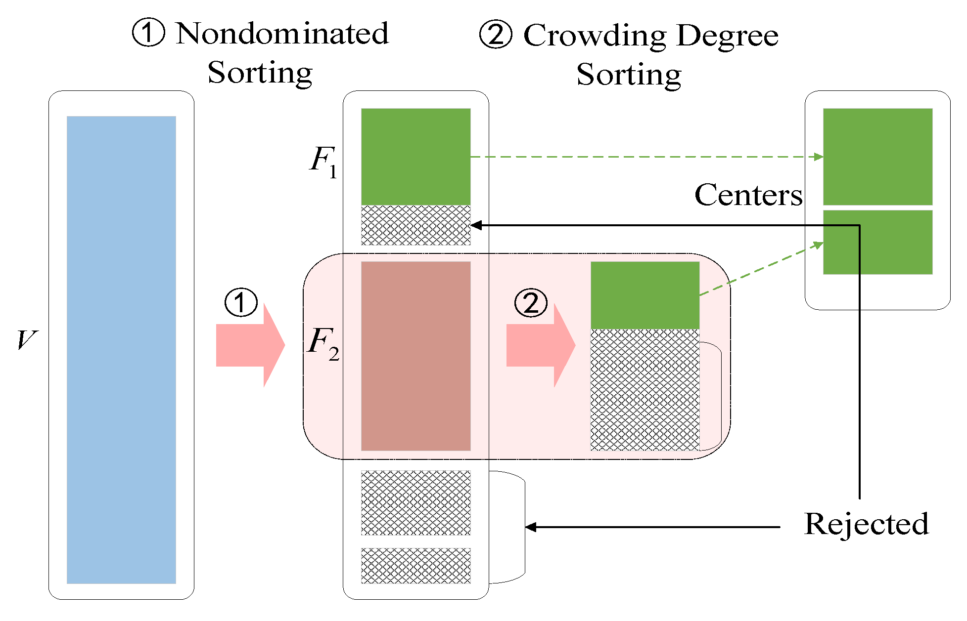
The specific selection process is shown in Figure 1. Firstly, based on non-dominated sorting, non-dominated sets for different layers are obtained. Then, when screening community centers, crowding non-dominated sorting method is used. Through two different sorting processes, all community centers are ultimately obtained.

Figure 1. Selection Process of Community Centers.

4.2. Process of Community Detection

After the community centers are determined, other nodes will be allocated to the center node a labeling algorithm. The community with center $c_i$ is denoted as ${\mathcal{C}}_i$, $i=1,2,\cdots ,s$. To achieve this, two parameters are defined to determine which set would be most suitable for a node to add in among ${\mathcal{C}}_1,{\mathcal{C}}_2,\cdots ,{\mathcal{C}}_s$.

Suppose that v is a node, H is a subset of V. The distance between v and H is defined as $dis(v,H)=\underset{w\in H}{min}\left\{dis(v,w)\right\}$. If $dis(v,H)=1$, then v has at least one neighbor node in H. Also note that for $v^{\prime }\in H$, $dis(v^{\prime },H)=0$.

If $dis(v,H)=1$, let $A(v,H)=N\left(v\right)\cap H$, which is called the attachment of v at H. $a(v,H)=\left|A\right(v,H\left)\right|$ is called the fitness of node v to set H, indicating the number of neighbors of node v in H. The greater the fitness, the tighter the connection between node v and set H.

The process of generating ${\mathcal{C}}_i$ is shown as Algorithm 2, which is mainly implemented through a labeling process. The input of the algorithm is graph G and the set of community centers $C=\{c_1,\cdots ,c_s\}$.

The label $p\left(v\right)$ represents the minimum distance from v to all communities. First, lines 1–8 regard each central node as a community and set the label values of the center nodes as 1, and that of other nodes as ∞.

Lines 9–24 assign all other nodes to the community with the highest fitness. $Belong$ records the community code with the highest fitness for each node. Lines 20–22 update the label values of the neighbor nodes.

Theorem 1. 

Suppose that G is a connected network. In Algorithm 1, if $R\ne \varnothing$, there is at least one $v\in R$ and ${\mathcal{C}}_i$, so that $dis(v,{\mathcal{C}}_i)=2$.

Proof. 

Assume that the theorem does not hold. For any $v\in R$, let $d=dis(v,{\mathcal{C}}_i)=\underset{1\le k\le s}{min}\left\{d(v,{\mathcal{C}}_k)\right\}$. According to the assumption, $2\le d<\infty$. So there is a path of length d, denoted as $v_1,\cdots ,v_d$, such that $v_1\in R,\cdots ,v_{d-1}\in R,v_d\in {\mathcal{C}}_i$. Then, $dis(v_{d-1},v_d)=1$ contradicts the hypothesis.    □

Algorithm 2 Community Detection

Input: $G=(V,E)$, C Output: Community division result ${\mathcal{C}}_1,\cdots ,{\mathcal{C}}_s$. 1: $p\left(v\right)=\infty$, $\forall v\in V$; 2: for $i=1$ to s do 3:     ${\mathcal{C}}_i$ = {$c_i\}$; 4:     $p\left(c_i\right)=0$; 5:     for $v\in N\left(c_i\right)\&p\left(v\right)\ne 0$ do 6:         $p\left(c_i\right)=1$; 7:     end for 8: end for 9: $R\leftarrow V\setminus \{c_1,\cdots ,c_s\}$; 10: while $R\ne \varnothing$ do 11:     for $v\in R\&p\left(v\right)=1$ do 12:         $Belong\left(v\right)=0$; 13:         for $i=1$ to s do 14:            if $a(v,{\mathcal{C}}_i)>Belong\left(v\right)$ then 15:                $Belong\left(v\right)=i$; 16:            end if 17:            ${\mathcal{C}}_{Belong\left(v\right)}={\mathcal{C}}_{Belong\left(v\right)}\bigcup \left\{v\right\}$; 18:         end for 19:         $R=R-v$; 20:         for $u\in N\left(v\right)\&p\left(u\right)\ne 0$ do 21:            $p\left(u\right)=1$; 22:         end for 23:     end for 24: end while 25: Output ${\mathcal{C}}_1,\cdots ,{\mathcal{C}}_s$.

Theorem 1 guarantees that the algorithm will not fall into a dead cycle for a connected graph. After the algorithm, all nodes are divided into s sets, that is, s communities are obtained. But when the network is disconnected, it is difficult to guarantee. In general, determining whether a network is connected also requires a lot of computation. So, we proposed a refinement for the algorithm.

4.3. Algorithm Refinement

In many cases, community-detection algorithms deal with networks that are not connected. If none of the nodes in a certain connected component is selected as the center of community, the nodes in that connected component cannot be classified into any community. At the same time, the algorithm will be stuck in a dead loop because there are always nodes that have not been classified into communities. In response to this scenario, algorithm augmentation and refinement have been undertaken. The fundamental idea involves recursively decomposing subgraphs not assigned to communities using the same method.

Firstly, the initial graph is subjected to community detection using Algorithm 2. After the number of iterations in Algorithm 2 exceeds the number of nodes, which means the algorithm enters a dead cycle, the algorithm terminates and outputs the set of undivided nodes, denoted as R. Take the nodes in R and edges between nodes to form a subgraph and apply Algorithm 2 for community detection within this subgraph. This process will continue recursively until all nodes are assigned to communities.

4.4. Overall Process

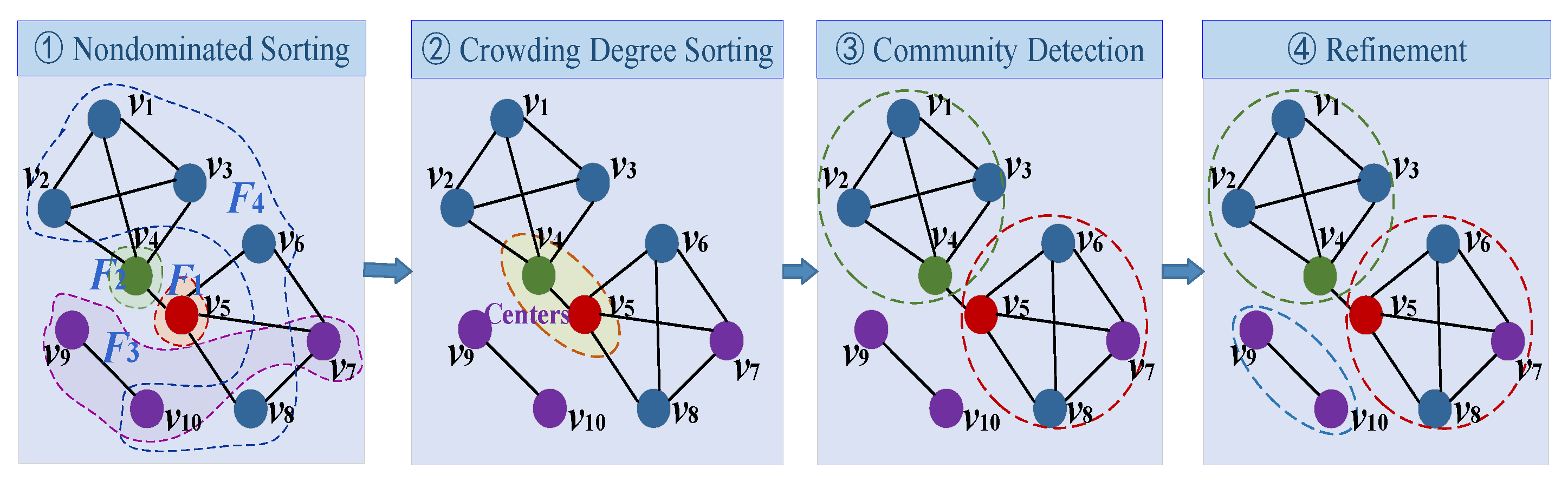
At this point, all the steps of this community-detection algorithm have been designed. The entire algorithm process includes four steps: node influence ranking, community center determination, community division and algorithm refinement. Given this, we denote the method proposed in this paper as the ICDR. The overall process of the proposed method is shown in Figure 2.

Figure 2. Overall process of the proposed method.

Step 1 divides the nodes in V into several layers according the influence vector. The influence matrix of the 10 nodes in the mini network shown in Figure 1 is as follows:

$$IV=\left(\begin{array}{ccc}0.75& 0.00& 0.39\\ 0.75& 0.00& 0.39\\ 0.75& 0.00& 0.39\\ 1.00& 0.33& 0.54\\ 1.00& 0.35& 0.54\\ 0.67& 0.00& 0.36\\ 0.75& 0.01& 0.39\\ 0.67& 0.00& 0.36\\ 1.00& 0.00& 0.11\\ 1.00& 0.00& 0.11\end{array}\right)$$

As can be seen from matrix $IV$, $v_5$ is a non-dominated node in V. So $F_1=\left\{v_5\right\}$. After removing $v_5$ from V, the non-dominated node in $V\setminus \left\{v_5\right\}$ is $v_4$. So $F_2=\left\{v_4\right\}$. Similarly, $F_3=\{v_7,v_9,v_{10}\}$. If we intend to divide all nodes into four layers, then $F_4=\{v_1,v_2,v_3,v_6,v_8\}$.

Step 2 determines the community centers by simultaneously considering node influence and crowding degree. First, $v_5$ is selected as the first center from $F_1$. Because $F_1$ only has one node, then we will consider $F_2$. Thus, $v_4$ is selected as the second center. If we only consider the non-dominated nodes in the first two layers, the selection process of community centers is over. If we consider the third layer of non-dominated nodes, $v_9$ or $v_{10}$ will be selected as the third center. The result in Figure 1 only considers the first two layers.

Step 3 divides the remaining nodes into various communities in sequence using the labeling algorithm. From Figure 1, we can see that ${\mathcal{C}}_1=\{v_5,v_6,v_7,v_8\}$ and ${\mathcal{C}}_2=\{v_1,v_2,v_3,v_4\}$. However, because nodes $v_9$ and $v_{10}$ are not connected to the other nodes, they will not be assigned to the above two communities.

Step 4 will modify the results if there are nodes that have not been divided into any community. We can see from Figure 1 that nodes $v_9$ and $v_{10}$ form a subgraph. Applying the same method, these two nodes will be divided into the same community.

In the above example, if we use the first three layers of nodes to determine the community centers, the refinement process will not be used, because we can run the algorithm to partition all nodes at one time.

4.5. Case Study

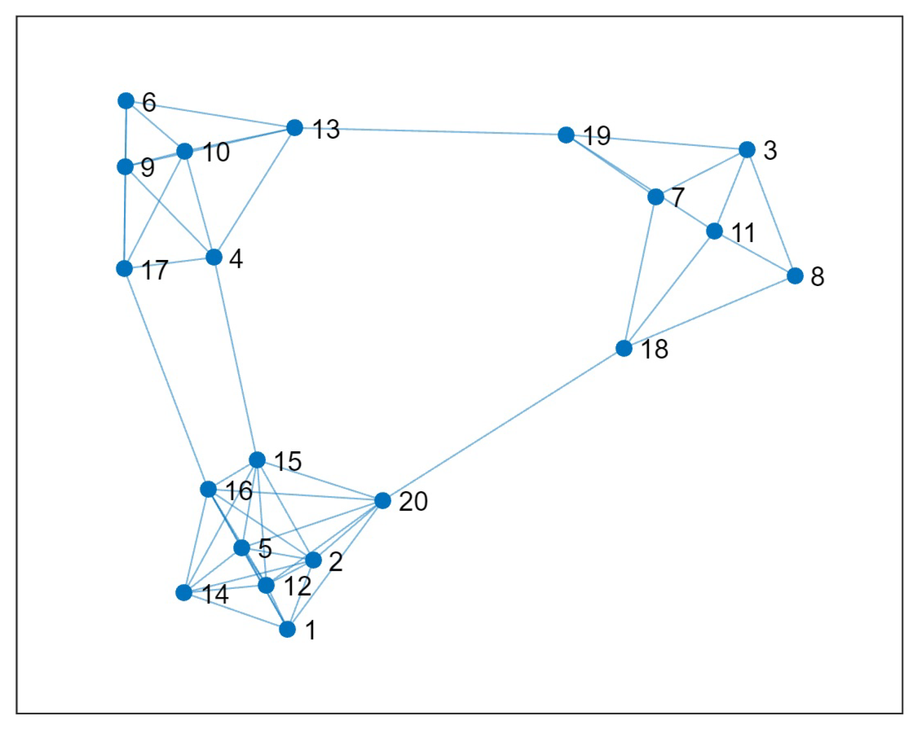
Random networks are also commonly used as test objects to evaluate algorithm performance [10]. We used a random network to illustrate the implementation process of our method and preliminarily verified its effectiveness. The network is shown in Figure 3, which contains 20 vertices and has three distinct community structures.

Figure 3. Example network.

Firstly, using node influence analysis, we can obtain the first layer of non-dominated nodes as $F_1=\{13,16,20\}$. From Figure 3, we can see that these three nodes do occupy important positions in the network. Similarly, the second layer of non-dominated nodes is $F_2=\{2,3,4,9,10,11,12,15,18,19\}$. The remaining nodes form the third layer $F_3$.

Using the selection method of community centers in this paper, we first select node 13 from $F_1$ as the community center. Since the crowding degree of nodes 16 and 20 is 0.5, we chose one of them as the community center. Suppose that we chose node 20. Next, we will make the selection in the second layer $F_2$. Taking into account both node influence and crowding degrees, we ultimately chose node 11 as the third community center. We can see from Figure 3 that these three nodes are exactly located in different communities, so the selected result is reasonable.

Then, we use labeling algorithms to sequentially partition all vertices into different communities.

Through this example, we can see that using only the nodes in the first layer to select community centers may result in biased results. Neglecting crowded degree can also lead to the consequences of having too many community centers.

5. Experiment

5.1. Experimental Subjects

To verify the effectiveness of our method, we selected seven classic real world networks for experiments, whose information is listed in detail in Table 1. Except for Dolphin amd Polbboks, all the data about these networks can be downloaded from the website http://snap.stanford.edu/data/ (accessed on 15 April 2024). Four of these networks have ground-truth community structures, but the remaining ones do not.

Table 1. Information of real world networks.

Network	Node Number	Edge Number	Community Number
Dolphin [39]	62	159	2
Polbooks [8]	105	441	3
Facebook	4039	88,234	/
Ca-GrQc	5242	14,496	/
Feather-lastfm-social	7624	27,806	/
DBLP	317,080	1,049,866	13,477
Amazon	334,863	925,872	75,149

5.2. Evaluation Indicator

Since four networks have ground-truth community structures, we adopt generalized Normalized Mutual Information ($NMI$) and $F1$ score to evaluate the performance of the proposed algorithm.

$NMI$: This indicator is used to measure the similarity between the detected community structures and the ground-truth community structures, whose definition is given as follows [40]:

$$NMT\left(\mathcal{C}\right|{\mathcal{C}}^{\prime })=\frac{1}{2}(H\left(\mathcal{C}\right|{\mathcal{C}}^{\prime })+H\left(\mathcal{C}\right|{\mathcal{C}}^{\prime }))$$

(6)

where $\mathcal{C}$ and ${\mathcal{C}}^{\prime }$ are two matrices that represent the detected community structures and the ground-truth community structures, respectively. The k-th rows ${\mathcal{C}}_k$ and ${\mathcal{C}}_k^{\prime }$ represent the node distribution of community $\mathcal{C}$ and ${\mathcal{C}}^{\prime }$, respectively. $H\left(\mathcal{C}\right)$ and $H\left(\mathcal{C}\right|{\mathcal{C}}^{\prime })$ are, respectively, the entropy of $\mathcal{C}$ and the conditional entropy of $\mathcal{C}$ with respect to ${\mathcal{C}}^{\prime }$.

The value of $NMT$ is between 0 and 1, and the higher the value, the better the performance of the algorithm.

F1 score: This indicator measures the closeness between the community structures discovered by the algorithm and the ground-truth community structures, which is given by the following formula [41]:

$$F1=\frac{1}{2}\left(\frac{1}{\left|\mathcal{C}\right|}\sum _{{\mathcal{C}}_i\in \mathcal{C}}Fit({\mathcal{C}}_i,{\mathcal{C}}_{\rho \left(i\right)}^{\prime })+\frac{1}{|{\mathcal{C}}^{\prime }|}\sum _{{\mathcal{C}}_j^{\prime }\in {\mathcal{C}}^{\prime }}Fit({\mathcal{C}}_{{\rho }^{\prime }\left(j\right)},{\mathcal{C}}_j^{\prime })\right)$$

(7)

where $\mathcal{C}$ and ${\mathcal{C}}^{\prime }$ are the detected and ground-truth communities, respectively. $\rho \left(i\right)=argma{x}_{j}Fit({\mathcal{C}}_i,{\mathcal{C}}_j^{\prime })$, ${\rho }^{\prime }\left(j\right)=argma{x}_{i}Fit({\mathcal{C}}_i,{\mathcal{C}}_j^{\prime })$ and $Fit({\mathcal{C}}_i,{\mathcal{C}}_j^{\prime })$ is the harmonic mean of Precision and Recall, i.e.,

$$F1({\mathcal{C}}_i,{\mathcal{C}}_j^{\prime })=2·\frac{precision({\mathcal{C}}_i,{{\mathcal{C}}^{\prime }}_j)·recall({\mathcal{C}}_i,{{\mathcal{C}}^{\prime }}_j)}{precision({\mathcal{C}}_i,{{\mathcal{C}}^{\prime }}_j)+recall({\mathcal{C}}_i,{{\mathcal{C}}^{\prime }}_j)}$$

where

$$precision({\mathcal{C}}_i,{\mathcal{C}}_j^{\prime })=\frac{\left|{\mathcal{C}}_i\cap {{\mathcal{C}}^{\prime }}_j\right|}{\left|{\mathcal{C}}_i\right|}$$

and

$$recall({\mathcal{C}}_i,{\mathcal{C}}_j^{\prime })=\frac{\left|{\mathcal{C}}_i\cap {{\mathcal{C}}^{\prime }}_j\right|}{\left|{{\mathcal{C}}^{\prime }}_j\right|}$$

Modularity is an indicator used to measure the degree of modularity in a network structure, which can help us evaluate the quality of community partitioning. The calculation formula for modularity is as follows [20]:

$$Q=\frac{1}{2m}\sum _{i,j}[a_{ij}-\frac{d\left(v_i\right)d\left(v_j\right)}{2m}]\delta ({\mathcal{C}}_i,{\mathcal{C}}_j)$$

(8)

where Q represents the modularity, m is the edge number of the network, $a_{ij}$ refers to the connection strength between nodes $n_i$ and $n_j$, $d_i$ and $d_j$, respectively, represent the degrees of nodes $v_i$ and $v_j$, ${\mathcal{C}}_i$ and ${\mathcal{C}}_j$ are the modules to which nodes $v_i$ and $v_j$ belong, and $\delta ({\mathcal{C}}_i,{\mathcal{C}}_j)$ equals 1 when ${\mathcal{C}}_i$ and ${\mathcal{C}}_j$ are equal; otherwise, it equals 0.

For all networks, we use modularity to measure the quality of community detection.

5.3. Experimental Results and Analysis

5.3.1. Correlation Analysis of Different Indicators

In order to verify the rationality of the centrality measurement indicators selected in this paper, we analyzed the correlation between different indicators. In addition to the three metrics we used, we also add the closeness centrality.

We generated 10 random networks, each containing three communities with varying numbers of nodes. Then, we calculate the node influence of each network separately. The final result is shown in Figure 4, in which, $C{C}_1$ refers to clustering coefficients and $C{C}_2$ refers to closeness centrality.

Figure 4. Correlation analysis of different indicators.

By analyzing the correlation, we find that there is a significant correlation between indicators $C{C}_1$ and $C{C}_2$. Combining other indicators and their correlations, we conclude that the three indicators we have chosen are quite reasonable.

5.3.2. Analysis of the Changing Trend of Non-Dominant Nodes

We obtain the number of non-dominated nodes $\eta$ for the Erdös–Rényi random graph of different node sizes n but fixed edge existence probability $p=0.3$.

From Figure 5, it could be seen that as the network size n continues to increase, the quantity of non-dominant nodes $\eta$ tends to grow roughly in a logarithmic fashion. To test the conjecture, a linear regression experiment is now performed on these data, with $logn$ as the predictor variable and $\eta$ as the response variable. The result of the linear regression model shows that the adjusted $R^2$ criterion is 0.9326 and the p-value for the F-statistic is $3.5\times {10}^{-15}$. This shows that our model explains the relationship between n and $\eta$ well. Overall, the number of non-dominated nodes is approximately linearly related to the log of the network size, i.e., $\eta \in O(logn)$. This result justifies our assumptions in the complexity analysis about the trend in the number of non-dominated nodes and the correctness of the algorithm’s complexity in the average case.

Figure 5. The changing trend of non-dominated nodes with network size.

5.3.3. The Community-Detection Results of Our Method

We used the method in this paper to divide the selected network into communities, and visualized partitioning results are shown as Figure 6 and Figure 7, in which different colors represent different communities. It should be noted that due to the large number of networks DBLP and Amazon, we are unable to display the detection results of the entire network, but only visualize the results of partial nodes (${10}^4$). However, the entire network was divided in the experiment.

Figure 6. Community-detection results for small real world networks. (a) Dolphin; (b) Polbooks.

Figure 7. Community-detection results for real world networks. (a) Facebook; (b) Ca-GrQc; (c) Feather-lastfm-social; (d) DBLP; (e) Amazon.

5.3.4. Comparison with Other Methods

To verify the effectiveness of the proposed algorithm, three classic community-detection algorithms are selected to compare with the algorithm proposed in this paper (ICDR): Girvan’s algorithm [8], CIDLPA [28] and CNLLP [20]. The final results of these four algorithms on four networks with ground-truth community structures are listed in Table 2.

Table 2. $NMI$ and $F1$ score of different methods on two networks.

Network	Girvan’s Algorithm		CIDLPA		CNLLP		ICDR
	NMI	F1 Score	NMI	F1 Score	NMI	F1 Score	NMI	F1 Score
Dolphin	0.521	0.631	0.489	0.526	0.637	0.674	0.889	0.982
Polbooks	0.535	0.628	0.612	0.634	0.482	0.491	0.507	0.775
DBLP	0.274	0.335	0.316	0.347	0.336	0.453	0.492	0.523
Amazon	0.336	0.387	0.353	0.416	0.373	0.584	0.452	0.632
Average	0.305	0.361	0.335	0.382	0.355	0.519	0.396	0.535

From Table 2, it can be seen that among the four comparative algorithms, our method (ICDR) achieves the highest $NMI$ value and $F1$ score in all networks. Among the other three algorithms, CNLLP is superior to CIDLPA, while CIDLPA is superior to Girvan’s algorithm. The experimental results fully demonstrate the superiority of the proposed method. In addition, all algorithms have better $F1$ scores than $NMI$ values. Moreover, all algorithms achieve better results in network Amazon compared to network DBLP.

The results on modularity for all networks are listed in Table 3.

Table 3. Modularity of different methods on all networks.

Network	Girvan’s Algorithm	CIDLPA	CNLLP	ICDR
Dolpin	0.501	0.592	0.384	0.374
Polbooks	0.518	0.563	0.566	0.450
Facebook	0.463	0.624	0.635	0.688
Ca-GrQc	0.524	0.536	0.572	0.684
Feather-lastfm-social	0.455	0.463	0.416	0.633
DBLP	0.574	0.642	0.682	0.674
Amazon	0.636	0.725	0.711	0.791
Average	0.530	0.598	0.603	0.665

From Table 3, it can be seen that the overall modularity obtained by our method is the highest, and our results are the best for most networks. The experimental results indicate that the community-detection method proposed in this paper can effectively reveal the community structure of the network.

6. Conclusions

Community structure is an important feature of complex networks. Mining communities can help analyze the structural features and functions of complex networks, and therefore has important theoretical and practical significance. Although various community-partitioning methods have been proposed, most of them often rely on the selection of seed nodes.

In view of this, this article proposes a complex network community-partitioning method based on node influence analysis. Firstly, this article uses Pareto dominance to divide nodes into several Zeng. Then, we use node influence and crowding to determine the community center. Finally, we use a labeling algorithm to divide the network into several communities. Finally, the method proposed in this article is applied to several practical networks. The comparison results with other methods demonstrate the effectiveness of this method.

Although the proposed method can effectively improve the efficiency and accuracy of community detection, there are also some insufficiencies. Firstly, the determination of some parameters involved in the algorithm still needs to be carefully studied. At present, we mainly rely on experimental analysis to determine these parameters, and have not conducted an in-depth analysis from a theoretical perspective. Secondly, the effectiveness of the proposed method still needs to be promoted and applied in more practical networks in order to comprehensively verify its performance.