Dynamic Spatiotemporal Correlation Graph Convolutional Network for Traffic Speed Prediction

Abstract

Accurate and real-time traffic speed prediction remains challenging due to the irregularity and asymmetry of real-traffic road networks. Existing models based on graph convolutional networks commonly use multi-layer graph convolution to extract an undirected static adjacency matrix to map the correlation of nodes, which ignores the dynamic symmetry change of correlation over time and faces the challenge of oversmoothing during training iterations, making it difficult to learn the spatial structure and temporal trend of the traffic network. To overcome the above challenges, we propose a novel multi-head self-attention gated spatiotemporal graph convolutional network (MSGSGCN) for traffic speed prediction. The MSGSGCN model mainly consists of the Node Correlation Estimator (NCE) module, the Time Residual Learner (TRL) module, and the Gated Graph Convolutional Fusion (GGCF) module. Specifically, the NCE module aims to capture the dynamic spatiotemporal correlations between nodes. The TRL module utilizes a residual structure to learn the long-term temporal features of traffic data. The GGCF module relies on adaptive diffusion graph convolution and gated recurrent units to learn the key spatial features of traffic data. Experimental analysis on a pair of real-world datasets indicates that the proposed MSGSGCN model enhances prediction accuracy by more than 4% when contrasted with state-of-the-art models.

1. Introduction

Traffic prediction is the core of modern Intelligent Transportation Systems (ITS). By collecting massive data to train and predict, immediate and precise predictions of traffic conditions can effectively assist transportation agencies in shaping their traffic strategies [1], improve road operation efficiency, and reduce the occurrence of urban road congestion and accidents.

Traffic prediction is based on historical records of multiple nodes distributed in the road network to predict future traffic conditions [2]. Nevertheless, as a result of the uneven configuration of the city’s road network structure, traffic flow data have complex temporal and spatial correlations. There are currently several issues in research in this area:

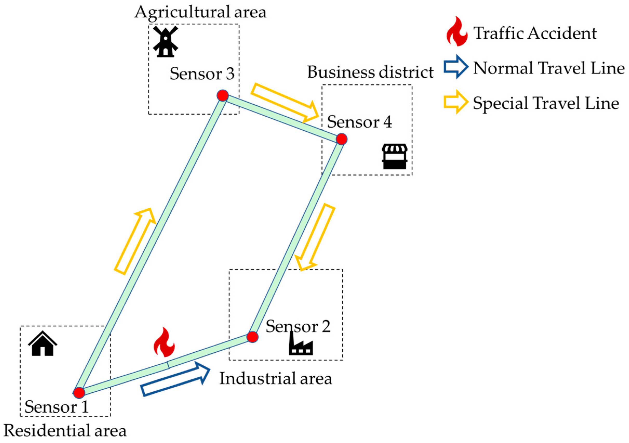
• Dynamic correlation between nodes. In previous studies, the correlation between nodes was often described using a static adjacency matrix, but in reality, the relationship among intersections within the traffic grid fluctuates over time. As shown in Figure 1, residents departing from a residential area to work in an industrial area often choose the route marked with a blue arrow due to its shorter distance. However, if a traffic accident occurs on this section, rendering it impassable, residents would be forced to choose the route marked with a yellow arrow to reach the industrial area. During this process, the originally strong correlation between nodes 1 and 2 would weaken or even become irrelevant. Therefore, learning the dynamic spatiotemporal correlations between nodes is very necessary.
• Oversmoothing problem of graphs. Although existing models have achieved relatively good results in traffic prediction using deep graph neural networks, deep graph neural networks gradually lose the graph structure and node feature information, leading to a decline in network performance. Therefore, it is necessary to forget irrelevant information layer by layer progressively.
• Long-term temporal feature extraction. Traffic data are not only influenced by short-term traffic conditions but also by long-term time dependence, such as people using a certain road to commute to work and returning home at the end of the day. On workdays, traffic congestion on the road significantly increases during morning and evening rush hours. However, on weekends or holidays, as most people do not go to work, the traffic flow on this road will be reduced and congestion will be significantly reduced. Therefore, observing the traffic data of this road over a long period will reveal clear cyclical changes in traffic flow and congestion.

Figure 1. Spatiotemporal correlation between road network nodes.

At present, there have been many studies on traffic prediction, but these methods still cannot account for the dynamic correlations between traffic nodes and complex spatiotemporal features. In these models, CNN [3] and GCN [4] are commonly used to extract spatial features from traffic data. However, the structure of traffic networks often exhibits asymmetric and irregular properties, and the CNN is limited by its inability to process non-Euclidean data. Therefore, the GCN has been subject to deeper investigation for handling traffic data, but deep GCN networks suffer from oversmoothing issues. Existing models often adopt residual connections to mitigate the oversmoothing issue, but this can increase the dependency between layers, resulting in an inability to learn sufficiently useful feature representations. Additionally, to learn temporal features, the Recurrent Neural Network (RNN) [5] and its variants are typically used, whereas TCN [6] has a better ability to learn long-term temporal features through the use of causal convolutions and dilated convolutions. However, in typical models, using only a single TCN is incapable of capturing the multi-level temporal features and patterns in the data [7].

Additionally, many recent models have adopted the self-attention mechanism from the Transformer architecture to enhance the processing efficiency of long sequential data and effectively capture the spatiotemporal correlations in the road network. Although this method is more effective at capturing the dynamic spatiotemporal correlations of the road network compared to static adjacency matrices, when dealing with missing or sparse sensor data within traffic flow data, the attention mechanism within the Transformer architecture may not fully utilize local information. Moreover, this approach is prone to overly concentrating attention on certain nodes while neglecting important information, which can lead to a decrease in prediction performance [8].

Therefore, to solve the above problems, this study proposes the MSGSGCN model. The TRL module is used to learn the temporal information in traffic data, and the GGCF module is built by combining gated fusion with an adaptive graph diffusion network to learn the spatial information in the traffic data. The NCE module has been designed to learn the hidden spatiotemporal correlation between nodes. Our main contributions are as follows:

• The NCE module is constructed in this paper to learn the dynamic spatiotemporal correlation between nodes using the matrix dot product after linear transformation and the multi-head self-attention mechanism.
• The time residual learner module is designed to learn long-term sequence information in traffic data, while the gated graph convolutional fusion module is used to effectively learn spatial information in traffic data and filter out useless information during the iterative process.
• This study leverages two authentic traffic datasets, METR–LA and PEMS–BAY, to validate the predictive performance of the novel MSGSGCN model presented. The empirical findings indicate that the model outshines eight reference models in various forecasting challenges.

The subsequent sections of this paper are structured as follows. Section 2 introduces classic methods for traffic prediction. Section 3 introduces the problem definition and the construction of the MSGSGCN model. Section 4 compares the performance of the proposed model with eight classical models on the METR–LA and PEMS–BAY datasets. Section 5 discusses the limitations of the model and future prospects.

2. Related Work

2.1. Traffic Speed Prediction with Classical Statistical Models

The traffic speed prediction problem can be regarded as a time series prediction problem. Ahmed [9] first applied the autoregressive integrated moving average (ARIMA) model, a time series prediction model, to the traffic-prediction problem. However, the ARIMA model assumes that the data are stable and exhibit linear relationships, while actual traffic data consist of various complex nonlinear relationships [10,11,12]. In response to this limitation, Williams et al. [13] considered the influence of upstream sensors on downstream sensors and proposed a seasonal autoregressive moving average model for discrete interval traffic flow data prediction. They demonstrated that this model can be applied to actual traffic data. However, the model assumes that the influence from upstream to downstream is fixed and stable, failing to capture the dynamic changes that often occur between upstream and downstream traffic. These statistical models, including ARIMA and the seasonal autoregressive moving average model, assume that traffic data are stable and overlook the presence of complex nonlinear relationships in actual traffic data [14,15,16].

2.2. Traffic Speed Prediction with Traditional Machine Learning

Due to the limitations of traditional statistical models, researchers have turned to machine learning models for traffic data processing and prediction. Compared to traditional statistical models, machine learning models have shown better capabilities in addressing the uncertainty and nonlinearity of traffic data. They possess stronger abilities in modeling nonlinear relationships, adaptability, flexibility, data processing, handling large-scale data, and learning comprehensive features. These advantages enable machine learning models to perform better in complex tasks such as traffic prediction.

The most representative of them is the K-nearest neighbor (KNN) algorithm. Davis et al. [17] constructed the KNN traffic-prediction model for the first time, but the calculation cost was not ideal in the calculation process, and the operation efficiency was not ideal. Another machine model used in traffic prediction is the support vector machine (SVM) [18], but it is still difficult to find the optimal parameters when dealing with a large amount of data, and the training efficiency and accuracy of the model are not high.

With the improvement in intelligent road detection equipment, the scale of traffic flow data is growing rapidly. However, traditional machine learning methods cannot handle these large-scale datasets well because they struggle to capture complex spatiotemporal correlations in the data [19,20]. In addition, these models usually adopt shallow architectures and require manual feature selection, and these problems make it difficult to cope with the traffic-prediction task in big data scenarios.

2.3. Traffic Speed Prediction with Deep Learning

The breakthrough of deep learning within computer vision [21] and natural language processing [22] has captured the interest of those researching transportation. Because deep learning technology can capture its hidden characteristics from raw data [23], it overcomes the need for manual parameter setting in traditional machine learning methods, which makes deep learning technology able to simulate complex spatiotemporal patterns in traffic prediction. In recent years, deep learning-based methods have been widely used in the field of transportation and can achieve excellent results in many traffic-prediction tasks.

The purpose of traffic prediction with deep learning techniques is to learn the spatiotemporal correlation in the data. Therefore, deep learning-based traffic-prediction models are typically segregated into two parts: one to model the temporal relationship and the other to model the spatial relationship.

In the early days of using deep learning techniques to deal with traffic-prediction problems, RNN was widely used to extract temporal dependencies in traffic data. By introducing recurrent connections inside the network, RNN can handle modeling and prediction tasks for sequential data, including traffic flow, speed, and congestion. However, the traditional RNN suffers from problems such as “vanishing gradient” and “exploding gradient”, which limit its performance in modeling long-term dependencies [24]. To overcome these problems, Long Short-Term Memory (LSTM) [25,26] and Gated Recurrent Unit (GRU) [27,28] have been introduced into the traffic-prediction task. LSTM and GRU add a gating mechanism to RNN, which can better capture long-term dependencies.

The CNN [29] is also widely used to extract spatial dependencies from traffic data. CNN can effectively capture spatial features in traffic data through convolution operations; however, traditional CNN is designed based on image data with Euclidean structure and cannot be directly applied to deal with spatial dependencies in traffic data. To solve this problem, the GCN [30,31] has been proposed to deal with data with non-Euclidean structures, such as traffic networks. The GCN can perform convolution operations on the graph structure to extract the feature representation of nodes by aggregating their neighbor information. Because the GCN performs very well in dealing with irregular graph data, a large number of subsequent studies have been carried out based on graph neural networks.

To more effectively extract spatiotemporal features in traffic data, the T-GCN [32] uses GRU and GCN to capture spatiotemporal correlations but still requires a pre-constructed adjacency matrix. The STGCN [33] combines convolutional networks and graph convolutional networks to form spatiotemporal graph convolutions, but it is difficult to capture long-term dependent features. On this basis, the ASTGCN [34] divides time series into adjacent, daily, and weekly features and adds spatiotemporal attention mechanisms but still cannot model dynamic graph data. The DCRNN [35] simulates spatial dependence using diffusion convolutional recurrent neural networks, but it is easy to overlook global graph structure information. Graph WaveNet [36] uses gated units to control information flow based on the DCRNN model but does not consider spatiotemporal correlations between nodes. The STSGCN [37] constructs a local spatiotemporal graph and stacks numerous spatiotemporal processing layers for feature manipulation, but the computational complexity is relatively high. Although these models consider the spatiotemporal characteristics of traffic data, the fusion of spatiotemporal features is not ideal, and the spatiotemporal relationships between road network nodes have not been well explored. Table 1 shows a comparison of classic spatiotemporal models.

Table 1. Comparison of classic spatiotemporal models.

Model Type	Model	Advantage	Disadvantage
Classical Statistical Model	ARIMA [9]	Earlier models for dealing with time series problems.	Struggles to handle complex nonlinear issues.
Traditional Machine Learning	KNN [17]	Easy to understand and implement.	Unable to handle high-dimensional data.
	SVM [18]	Can handle medium- to small-sized datasets.	Computational performance is suboptimal when handling large datasets.
Classic Deep Learning Method	T-GCN [32]	Spatiotemporal characteristics of traffic data are considered.	A pre-built adjacency matrix is required.
	STGCN [33]	The receptive field of CNN is improved.	Difficult to capture long-term dependency features.
	ASTGCN [34]	Time series is divided into neighboring features, daily features, and weekly features.	It cannot simulate dynamic graph data.
	DCRNN [35]	Traffic movement is modeled as a process of dispersion.	Global graph structure information is ignored.
	Graph WaveNet [36]	The gating unit is used to control the information flow.	The spatiotemporal correlation between nodes is not considered
	STSGCN [37]	Combines adjacent time steps into a new adjacency matrix.	High complexity.
The proposed model.	MSGSGCN	Learns the dynamic spatiotemporal correlations and long-term temporal patterns in the road network.	The impact of external factors in the real world, such as weather and holidays, is not considered.

Compared to these models, the MSGSGCN considers the spatiotemporal heterogeneity of traffic data, dynamically learns the spatiotemporal correlations between nodes, and efficiently captures long-distance spatiotemporal features to achieve more accurate prediction accuracy.

3. Methodology

3.1. Problem Definition

The traffic-prediction problem is to predict future traffic data based on historical traffic data. This task can be viewed as a forecasting challenge for multivariate time series, enriched by some pre-existing understanding. The graph structure G is the prior knowledge describing the spatial structure of the road network.

Definition 1. 

This paper defines a certain road network as G = (V, E, A), where $\left|\mathit{V}\right|=N$ represents different nodes of the road network (e.g., sensors) and E represents edges, which represent the connection relationship between nodes. $\mathit{A}\in {\mathbb{R}}^{N\times N}$ is an adjacency matrix representing the spatial relationship between nodes (e.g., spatial distance or adjacency).

Definition 2. 

The formula definition of traffic prediction can be expressed as follows: given P time steps of historical data $\mathit{{\rm X}}=({\mathit{X}}^1, {\mathit{X}}^2, \cdots , {\mathit{X}}^P),\mathit{{\rm X}}\in {\mathbb{R}}^{N\times P\times F},$ predict T time steps of future data $\mathit{Y}=({\mathit{Y}}^{P+1}, {\mathit{Y}}^{P+2}, \cdots , {\mathit{Y}}^{P+T}), \mathit{Y}\in {\mathbb{R}}^{N\times T\times F^{’}}$, and $F^{’}$ and $F$ denote the historical and predicted feature dimensions, respectively.

3.2. Overview

In this section, the overall architecture of MSGSGCN is introduced initially, followed by an introduction to the structure of the related components of the model.

The architecture of the model proposed in our study is depicted in Figure 2, including the NCE module to assess the interconnectivity among nodes and several spatiotemporal modules to capture the spatiotemporal characteristics of traffic data. Each module contains a TRL module for capturing long-distance temporal dependencies, as well as a GGCF module for spatial information learning and spatiotemporal fusion.

Figure 2. Overall architecture. The light yellow region is used to learn the dynamic correlations between traffic nodes. The light green region is used to learn the spatiotemporal features in the traffic data, specifically, the yellow module is for learning temporal features, while the gray region is for learning spatial features. Historical data from the past P time steps are inputted to MSGSGCN through linear transformation to obtain the predictions for T time steps.

3.3. Node Correlation Estimator

There is a spatiotemporal correlation among different nodes in a road network. It is crucial to learn the correlation between each node and explain its causal relationship for accurate traffic prediction. For instance, Dynamic Time Warping (DTW) [38] measures the similarity between two time series by calculating the minimum distance between them, but it has low computational efficiency and suboptimal performance.

While the standard self-attention module can also calculate the spatiotemporal correlation between nodes, it faces the issue of sparse attention distribution, which often leads to the model overlooking some important information. Therefore, in the NCE model, by integrating a similarity evaluation module that is primarily composed of dot product operations, the ability of the model to learn key information can be enhanced, avoiding an overly concentrated attention distribution on certain nodes.

The model first processes the input signal $\mathit{{\rm X}}\in {\mathbb{R}}^{N\times P\times F}$ through a linear layer and smooths the two linear processing results with BatchNorm and ELU activation functions. Then, it passes them through a separate linear layer, respectively, and multiplies the resulting matrices in parallel, activating the result with LeakyRelu. The multiplied result is then input into the multi-head self-attention module for further processing. In the multi-head self-attention module, three subspaces can be generated, including Query vector Q, Key vector K, and Value vector V. The process of learning peripheral node features can be expressed as follows:

$$\mathit{Q}=\mathit{X}{\mathit{W}}^Q, \mathit{K}=\mathit{X}{\mathit{W}}^K, \mathit{V}=\mathit{X}{\mathit{W}}^V$$

(1)

where the relevance is calculated by computing Q and K for the dot product, and softmax is used to calculate the attention weight:

$$Attention(\mathit{Q},\mathit{K},\mathit{V})=softmax\left(\frac{\mathit{Q}{\mathit{K}}^T}{\sqrt{d_k}}\right)\mathit{V}$$

(2)

where $d_k$ represents the dimension size of K. This division is called scaling, and it helps to stabilize the gradients during model training.

To enhance the fitting performance, this paper further employs multi-head self-attention, concatenating individual attention results to obtain the following:

$${\mathit{X}}_{multi}=Concat \left({\mathit{head}}_1,\dots ,{ \mathit{head}}_h\right){\mathit{W}}_a$$

(3)

where ${ \mathit{h}\mathit{e}\mathit{a}\mathit{d} }_i=Attention \left({\mathit{Q}}_i,{\mathit{K}}_i,{\mathit{V}}_i\right)$ resents the attention weight calculation results of different heads. When using more heads to jointly focus on inputs from different representation subspaces, the model can learn more diverse latent information.

After using multi-head self-attention, the results are normalized by a layer norm, and the learning results of node correlation are multiplied with the original input Hadamard through the linear layer, which is equivalent to adding the embedding of node correlation to the original input and constructing the residual structure with the original input. Figure 3 shows the structure of the Node Correlation Estimator.

Figure 3. Extraction of dynamic spatiotemporal correlations in road networks. The blue module represents linear transformation, and the orange region represents activation function. $\otimes$ indicates element-wise product. $⨁$ indicates element-wise addition.

3.4. Spatiotemporal Module

3.4.1. Temporal Residual Learner

One-dimensional temporal convolution makes it easy to forget important information when dealing with long-term time dependencies. RNN can capture long-term dependency but has large computational consumption and is difficult to parallelize. Compared with the traditional model, the convolution method used by TCN is dilated causal convolution. The improved model has the advantages of parallel computing, long-term dependence modeling, stable gradient propagation, and flexibility in processing time series data, which can flexibly and effectively learn long-term time series features.

Although the TCN has advantages in extracting long-term temporal features, a single TCN may find it difficult to capture subtle distinctions in long-term temporal dependencies. However, combining multiple TCNs can significantly enhance the model’s learning ability, thereby capturing features and patterns at multiple levels of the data. Therefore, this paper employs multiple TCNs to construct a residual structure to capture deeper temporal characteristics. The overall framework is shown in Figure 4.

Figure 4. Long-term temporal pattern learning. The brown region represents TCN operation with input as ${\mathit{X}}_{multi}$.

The expression for the Temporal Residual Learner can be expressed as follows:

$${\mathit{X}}^{filter}=Tconv\left({\mathit{X}}_{multi}\right)$$

(4)

$${\mathit{X}}^{gate}=Tconv\left({\mathit{X}}_{multi}\right)$$

(5)

$${\mathit{X}}^{res}=Tconv\left({\mathit{X}}_{multi}\right)$$

(6)

$${\mathit{X}}^{temp}=LeakyReLU\left({\mathit{X}}^{res}+ELU\left({\mathit{X}}^{filter}\right)\otimes ELU\left({\mathit{X}}^{gate}\right)\right)$$

(7)

where $Tconv$ denotes the dilated causal convolution operation, and $\otimes$ denotes the Hadamard product. Compared to a single TCN module, the TRL module can more effectively learn time features of different layers and models through residual connections of multiple TCNs and reduce gradient attenuation to enhance the model’s ability to learn long-term time features.

3.4.2. Adaptive Diffusion Graph Convolution Network

The advantage of a graph neural network is that it can effectively learn non-European spatial structure, but ordinary graph convolution is only suitable for undirected graph structure. Suppose input signal $\mathit{X}\in {\mathbb{R}}^{N\times F}$ and an adjacency matrix $\mathit{A}\in {\mathbb{R}}^{N\times N}$. The diffusion graph convolution proposed by Li et al. [35] can effectively learn the directed graph structure:

$$\mathit{Z}=\sum _{k=0}^K {\mathit{P}}_f^k\mathit{X}{\mathit{W}}_k+{\mathit{P}}_b^k\mathit{X}{\mathit{W}}_k$$

(8)

where the forward transition matrix is ${\mathit{P}}_f=\mathit{A}/rowsum\left(\mathit{A}\right)$, the backward transition matrix is ${\mathit{P}}_b={\mathit{A}}^{\mathrm{T}}/rowsum\left({\mathit{A}}^{\mathrm{T}}\right)$, and K is the diffusion order.

In addition, in the real world, many graph data are dynamic, nodes and edges may change over time, and a fixed graph structure cannot directly adapt to this dynamic nature. In order to make up for the shortcomings of the fixed adjacency matrix and reduce the impact of missing data on prediction results, the adaptive adjacency matrix is introduced:

$${\tilde{\mathit{A}}}_{adp}=SoftMax\left(ReLU\left({\mathit{E}}_1{\mathit{E}}_2^{\mathrm{T}}\right)\right)$$

(9)

where ${\mathit{E}}_1$, and ${\mathit{E}}_2^{\mathrm{T}}$ are learnable matrices. Finally, graph convolution can be expressed as follows:

$$\mathit{Z}=\sum _{k=0}^K {\mathit{P}}_f^k\mathit{X}{\mathit{W}}_{k1}+{\mathit{P}}_b^k\mathit{X}{\mathit{W}}_{k2}+{\tilde{\mathit{A}}}_{adp}\mathit{X}{\mathit{W}}_{k3}$$

(10)

where ${\mathit{W}}_{k1},{\mathit{W}}_{k2}, {\mathit{W}}_{k3}$ are the learnable parameters, respectively.

3.4.3. Gated Graph Convolutional Fusion

Although deep GCN networks have a stronger capability in extracting spatial features and can integrate more information between distant nodes, capturing long-distance dependencies between nodes, they suffer from the oversmoothing problem, where with increasing layers, different nodes tend to exhibit similar features, losing distinctiveness. Therefore, this paper employs a recurrent gating mechanism to control the propagation of information in deep GCNs by discarding irrelevant information layer by layer to enhance the model’s ability to mine deep spatial features. This approach effectively avoids excessive dependencies between layers compared to ordinary residual methods.

As shown in Figure 5, this paper uses a gating structure similar to GRU in the process of information transmission. By gating the control input and the processing results of the adaptive graph diffusion network, GCN can reduce the transmission of useless information and improve the calculation accuracy in the process of information transmission.

Figure 5. Spatiotemporal feature fusion. The blue module represents gate control unit, GCN is the diffusion graph convolution operation mentioned earlier.

The expression of Gated Graph Convolutional Fusion can be expressed as follows:

$$\mathit{z}=\sigma \left({\mathit{W}}_{zx}{\mathit{X}}^{temp}+{\mathit{W}}_{zg}\left[GCN\left({\mathit{X}}^{temp},\mathit{A}\right)\right]\right)$$

(11)

$$\mathit{r}=\sigma \left({\mathit{W}}_{rx}{\mathit{X}}^{temp}+{\mathit{W}}_{rg}\left[GCN\left({\mathit{X}}^{temp},\mathit{A}\right)\right]\right)$$

(12)

$$\mathit{s}=ReLU\left({\mathit{W}}_{sx}\left[GCN\left({\mathit{X}}^{temp},\mathit{A}\right)\right]+{\mathit{W}}_{sg}\left(\mathit{r}\ast {\mathit{X}}^{temp}\right)\right)$$

(13)

$$\mathit{h}=\mathit{z}\ast {\mathit{X}}^{temp}+\left(1-\mathit{z}\right)\ast \mathit{s}$$

(14)

where ${\mathit{X}}^{temp}$ denotes the processing result of the above TRL module, and $\left[GCN\right({\mathit{X}}^{temp},\mathit{A}\left)\right]$ denotes the Adaptive Diffusion Graph Convolution operation. $\sigma$ is the activation function Sigmoid.

Two gating units, $\mathit{z}$, and $\mathit{r}$, activated with Sigmoid, are used to control how the previous information is updated at the current time and to control whether the previous information should be ignored at the current time, respectively. Controlling the retention and update of information can help GCNs process spatial information faster and more efficiently, avoiding the oversmoothing issue caused by multiple graph convolutions and enabling the model to simulate the spatial structure of real road networks.

3.4.4. Loss Function

Use Mean Absolute Error (MAE) as the loss function, where $m$ represents the number of samples, $y_i$ and ${\widehat{y}}_i$ represent the actual value and the model predicted value, respectively.

$$\begin{array}{c}Loss=\frac{1}{m}\left({\displaystyle \sum _{i=1}^m} \left|y_i-{\widehat{y}}_i\right|\right)\end{array}$$

(15)

3.5. Training Process

During the training process, it is necessary to optimize all parameters in the MSGSGCN using gradient descent. In order to present the training process of the model more clearly, Algorithm 1 shows the training process of the model parameters.

Algorithm 1: Training process of MSGSGCN.

Input:$\mathrm{Training} \mathrm{set} {{\rm P}}_{train}$.    $\mathrm{Pre-defined} \mathrm{adjacency} \mathrm{matrix} \mathit{A}\in {\mathbb{R}}^{N\times N}$.    $\mathrm{Historical} \mathrm{data} \mathit{{\rm X}}=({\mathit{X}}^1, {\mathit{X}}^2, \cdots ,{\mathit{X}}^P),\mathit{{\rm X}}\in {\mathbb{R}}^{N\times P\times F}$. Output: Trained MSGSGCN model. Set model hyperparameters; repeat   $\mathrm{randomly} \mathrm{sample} \mathrm{a} \mathrm{batch} \left\{\mathit{X}, \mathit{Y}\right\}$$\mathrm{from} {{\rm P}}_{train};$   ${\mathit{X}}_{multi}$ ←$\mathit{{\rm X}}$ using Equations (1)–(3);   ${\mathit{X}}^{temp}$ ←${\mathit{X}}_{multi}$ using Equations (4)–(7);   $\mathit{h}$ ←${ \mathit{X}}^{temp}$ using Equations (11)–(14);   $\widehat{\mathit{Y}}$ ←$\mathcal{F}\left(\mathit{h}\right)$ utilizes residual and linear transformations;   compute $\mathrm{L}\mathrm{oss}$ using Equation (15);   $\theta$←$\theta -\alpha {\nabla }_{\theta }\mathrm{L}\mathrm{oss}$ update learnable parameters using gradient descent; until reaching the stopping condition. Output the trained MSGSGCN model.

In Algorithm 1, $\theta$ represents the trainable parameters in the traffic-prediction model, with gradients denoted as ${\nabla }_{\theta }\mathrm{L}\mathrm{oss}$ and the learning rate as $\alpha$. The algorithm takes historical traffic data and a pre-defined adjacency matrix as inputs and iteratively learns to select the optimal model parameters for output.

4. Experiments

In this section, two datasets are employed to validate the performance of MSGSGCN. The casting details are provided below.

4.1. Datasets

This paper performs experiments on two highway datasets, METR–LA and PEMS–BAY [35]. METR–LA is provided by the Los Angeles City Transportation Bureau and the University of Southern California, and PEMS–BAY is from the Bay Area of California. The specific information is shown in Table 2.

Table 2. Dataset information.

Dataset	METR–LA	PEMS–BAY
Area	Los Angeles	Bay Area of California
Nodes	207	325
Time interval	5 min	5 min
Target	Speed	Speed
Start time	1 March 2012	1 January 2017
End time	27 June 2012	30 June 2017

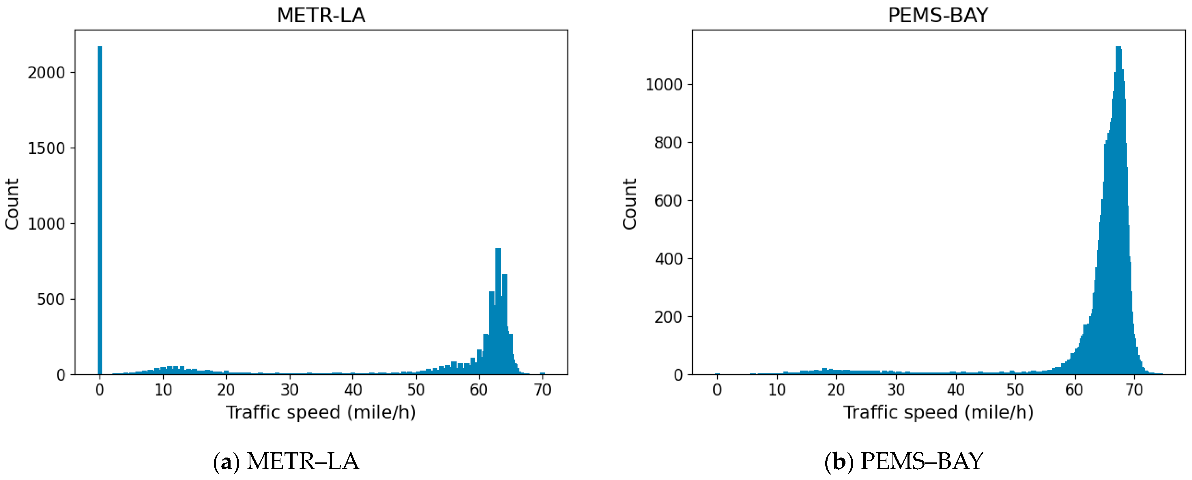
• METR–LA. The METR–LA dataset is an open dataset for traffic speed prediction. The dataset collects data from 207 sensors on the freeways of Los Angeles from March to June. Figure 6a presents the dataset through a visual graph.
  

  Figure 6. Traffic speed distribution in the dataset.
• PEMS–BAY. The PEMS–BAY dataset contains data collected from 325 nodes from January 2017 to June 2017. Figure 6b presents the dataset through a visual graph.

4.2. Experimental Setup

4.2.1. Data Splitting

The dataset was split into three parts for training, validation, and testing, following a proportion of 70%, 10%, and 20%, respectively. The training set was used to train the model, the validation set was used to adjust model hyperparameters and evaluate the model’s performance on unseen data, and the testing set was used to evaluate the model’s generalization ability on unknown data. The optimal model parameters were selected based on the minimum error on the validation set, and then the model was tested on the testing set.

4.2.2. Hyperparameter Settings

In the experiments, Pytorch 1.6.1 was used to implement the experiments on a graphics card with 8 GB memory; the graphics card used NVIDIA GeForce RTX 3070, the batch size was set to 64, Adam was used to optimize, and the learning rate was 0.001. The dropout rate was set to 0.3 to prevent overfitting. Note that the number of heads in the METR–LA dataset and PEMS–BAY dataset was set to 4.

4.3. Baseline Models and Evaluation Metrics

4.3.1. Evaluation Metrics

This study used four error metrics to evaluate the prediction effect of MSGSGCN. These are MAE, Mean Absolute Percentage Error (MAPE), Root Mean Square Error (RMSE), and Mean Hassanat Distance (MHD) [39]. Additionally, this study introduces the MHD as an evaluation metric in the ablation experiments, as it is less sensitive to outliers and better able to accurately assess model performance, where an MHD result closer to 0 indicates a more ideal outcome. It should be noted that the dataset used in this paper consists of vehicle speeds, which are all non-negative values. Therefore, a portion of the MHD formula used in the paper is specifically designed for non-negative values. The equations for MAPE, RMSE, and MHD are as follows:

$$\mathrm{M}\mathrm{A}\mathrm{P}\mathrm{E}=\frac{1}{m}\left(\sum _{i=1}^m \left|\frac{y_i-{\widehat{y}}_i}{y_i}\right|\right)$$

(16)

$$\mathrm{R}\mathrm{M}\mathrm{S}\mathrm{E}=\sqrt[2]{\frac{1}{m}\left(\sum _{i=1}^m {\left(y_i-{\widehat{y}}_i\right)}^2\right)}$$

(17)

$$\mathrm{M}\mathrm{H}\mathrm{D}=\left\{\begin{array}{c}\frac{\sum \left(1-\frac{1+min\left(y_i,{\widehat{y}}_i\right)}{1+max\left(y_i,{\widehat{y}}_i\right)}\right)}{m}, min\left(y_i,{\widehat{y}}_i\right)\ge 0\\ \frac{\sum \left(1-\frac{1+min\left(y_i,{\widehat{y}}_i\right)+\left|min\left(y_i,{\widehat{y}}_i\right)\right|}{1+max\left(y_i,{\widehat{y}}_i\right)+\left|min\left(y_i,{\widehat{y}}_i\right)\right|}\right)}{m}, min\left(y_i,{\widehat{y}}_i\right)<0\end{array}\right.$$

(18)

where the parameters and the loss mentioned in the previous context remain consistent.

4.3.2. Baseline Models

Eight traffic-prediction models are selected as baseline models to compare with the proposed model. In the experiments comparing with these baseline models, this paper references the parameter settings described in the baseline papers and relevant literature.

• ARIMA [9]. Integrating moving-average autoregressive models and using the difference to deal with time series problems.
• SVR [40]. Support vector regression, a commonly used time series analysis model.
• DCRNN [35]. Diffusion convolutional recurrent neural networks that learn spatiotemporal features using diffusion convolutions.
• STGCN [35]. Spatiotemporal convolutional models, combining graph convolutional layers and convolutional sequences to learn spatiotemporal features.
• ASTGCN [34]. Time is divided into three parts: adjacent, daily, and weekly.
• STSGCN [37]. Three consecutive adjacent time slices are constructed into a local spatial graph.
• CCRNN [41]. A hierarchical coupling mechanism is proposed to fuse the adjacency matrices of different layers.
• ADN-FA [42]. The model is based on an Attention Diffusion Network (ADN) [43], which is a decoder–encoder architecture and does not require any prior knowledge. ADN-FA improves upon the original Dot-product Attention (DA) in the ADN model by replacing it with Fast Linear Attention (FA).

4.4. Results

4.4.1. Comparative Experiment

Table 3 and Table 4 display the comparative results of the model on two datasets.

Table 3. Comparison experiments on the METR–LA dataset.

Data	Models	15 min			30 min			60 min
		MAE	RMSE	MAPE	MAE	RMSE	MAPE	MAE	RMSE	MAPE
METR–LA	ARIMA	3.99	8.21	9.60%	5.15	10.45	12.70%	6.90	13.23	17.40%
	SVR	3.39	8.45	9.30%	5.05	10.87	12.10%	6.72	13.76	16.70%
	DCRNN	2.77	5.38	7.30%	3.15	6.45	8.80%	3.60	7.60	10.50%
	STGCN	2.88	5.74	7.62%	3.47	7.24	9.57%	4.59	9.40	12.70%
	ASTGCN	4.86	9.27	9.21%	5.43	10.61	10.13%	6.51	12.52	11.64%
	STSGCN	3.31	7.62	8.06%	4.13	9.77	10.29%	5.06	11.66	12.91%
	CCRNN	2.85	5.54	7.50%	3.24	6.54	8.90%	3.73	7.65	10.59%
	ADN-FA	3.02	6.01	8.20%	3.56	7.30	10.22%	4.31	8.70	12.61%
	MSGSGCN	2.78	5.36	7.26%	3.14	6.32	8.67%	3.54	7.25	10.16%

Note: The bold data represents the best one within the same evaluation indicator.

Table 4. Comparison experiments on the PEMS–BAY dataset.

Data	Models	15 min			30 min			60 min
		MAE	RMSE	MAPE	MAE	RMSE	MAPE	MAE	RMSE	MAPE
PEMS–BAY	ARIMA	1.62	3.30	3.50%	2.33	4.76	5.40%	3.38	6.50	8.30%
	SVR	1.85	3.59	3.80%	2.48	5.18	5.50%	3.28	7.08	8.00%
	DCRNN	1.38	2.95	2.90%	1.74	3.97	3.90%	2.07	4.74	4.90%
	STGCN	1.36	2.96	2.90%	1.81	4.27	4.17%	2.49	5.69	5.79%
	ASTGCN	1.52	3.13	3.22%	2.01	4.27	4.48%	2.61	5.42	6.00%
	STSGCN	1.44	3.01	3.04%	1.83	4.18	4.17%	2.26	5.21	5.40%
	CCRNN	1.38	2.90	2.90%	1.74	3.87	3.90%	2.07	4.65	4.87%
	ADN-FA	1.48	3.04	3.05%	1.87	4.12	4.16%	2.34	5.22	5.72%
	MSGSGCN	1.33	2.84	2.80%	1.67	3.81	3.77%	1.97	4.53	4.61%

Note: The bold data represents the best one within the same evaluation indicator.

To better evaluate the performance of the model, this paper includes a range of base-line models: a statistical model ARIMA; a machine model SVR; classic spatiotemporal models like DCRNN, STGCN, ASTGCN, STSGCN; and recently popular encoder–decoder architecture models CCRNN and ADN-FA. The variety of baseline models helps us better assess our model’s improvements.

Using RMSE as the evaluation metric, on the METR–LA and PEMS–BAY datasets, MSGSGCN reduces the error by 45.2% and 30.3%, respectively, compared to the statistical model ARIMA, and by 47.3% and 36.0%, respectively, compared to the machine model SVR. Compared with classic spatiotemporal graph neural networks such as DCRNN, STGCN, and STSGCN, the reduction is 4.6%, 22.9%, and 37.8%, respectively, while on the PEMS–BAY dataset, the reduction is 4.4%, 20.4%, and 13.1%, respectively. Additionally, compared to the encoder–decoder structure-based ADN-FA model, there is also a reduction in error of 16.7% and 13.2%. Furthermore, Figure 7 presents the visualization comparison of model performance for prediction step lengths of 15, 30, and 60 min.

Figure 7. Comparison with baseline models in terms of MAE.

In Figure 7, it can be seen that as the prediction time steps increase, the prediction difficulty also increases, and the prediction errors of all models show an upward trend. However, the MSGSGCN still performs well in medium- and long-term prediction performance. Additionally, the experimental results also show that due to the limited processing ability of traditional machine models in handling realistic and complex traffic data, deep learning models generally outperform machine learning models, indicating that deep learning has stronger modeling ability in traffic speed prediction tasks. In addition, decoder–encoder-based models perform well in long-range prediction tasks, such as predicting for a 60 min time horizon. This is because this structure exhibits good parallelism, which provides significant advantages in handling longer time series data.

Compared to the proposed models, the listed baseline models still have shortcomings. STGCN and DCRNN have relatively weak modeling ability for long-term dependencies and suffer from gradient explosion problems. Although the ASTGCN captures the importance of spatiotemporal features using attention mechanisms, it cannot adaptively construct the graph structure. Although the STSGCN constructs a local spatiotemporal graph to learn spatiotemporal features of multiple time steps, its ability to model node dynamics is limited. Although the CCRNN constructs a hierarchical coupling mechanism, it still fails to effectively learn the correlation between nodes. Although the ADN-FA constructs a structure similar to a Transformer to learn long-distance temporal dependencies, the fusion of spatiotemporal features is not ideal. In contrast, the MSGSGCN learns the spatiotemporal correlation between nodes and deeply mines the long-term dependent temporal features and deep spatial features, resulting in good prediction performance.

4.4.2. Visualization

To provide a more intuitive understanding and evaluation of the model, Figure 8 features a well-crafted chart that visualizes the correlation between the model’s predicted results and the actual data points. To demonstrate the model’s generalization capability, we randomly selected 2 nodes from each dataset (nodes 5 and 16 from the METR–LA dataset and nodes 8 and 66 from the PEMS–BAY dataset) and depicted their comparative data across different time steps, showcasing the precision of the model’s predictions. The model fits the real data well and has a robust predictive ability for peaks and troughs in traffic, indicating that the model can effectively forecast variations in traffic data. Notably, the model does not attempt to overfit some noise in the data. For instance, in the METR–LA dataset, there are some outliers present in the original data; hence, outlier values were replaced with 0 during data preprocessing. Nonetheless, our model does not force-fit to noisy data and can predict traffic flows accurately.

Figure 8. Visualization of the METR–LA and PEMS–BAY datasets. (a) Visualization of node (sensor) 5 in the METR–LA dataset. (b) Visualization of node (sensor) 16 in the METR–LA dataset. (c) Visualization of node (sensor) 8 in the PEMS–BAY dataset. (d) Visualization of node (sensor) 66 in the PEMS–BAY dataset.

4.4.3. Ablation Study

To assess the efficiency of different modules, a comparison of the following variants was conducted using the METR–LA dataset.

• NNCE. The node correlation estimator module is removed, and the feedforward network is used instead.
• NTRL. The TRL module is removed, using only a single TCN with ELU activation.
• NGC. The Gated Graph Convolutional Fusion module is removed, and only Adaptive Diffusion Graph Convolution is used.

Table 5 presents the average results of the multi-step ablation experiments, where MSGSGCN has the lowest errors in 15 min, 30 min, and 60 min time-step predictions, indicating that the addition of the NCE module enables the model to better learn the dynamic correlations among nodes and improve the accuracy. Removing the TRL module significantly reduces the model’s ability to learn long-term traffic data, while removing the Gated Graph Convolutional Fusion module leads to the inclusion of too much useless information during the computation process, making it difficult for the model to learn useful information and hence decreasing the prediction accuracy. Furthermore, the MHD evaluation results show that the MSGSGCN maintains good predictive performance across all forecast time steps, indicating that the model possesses a robust noise resistance capability. To illustrate the accuracy improvement more clearly, Figure 9 shows the multi-step error value change.

Table 5. Comparison of ablation experiments.

Ablation	15 min			30 min			60 min
	MAE	RMSE	MHD	MAE	RMSE	MHD	MAE	RMSE	MHD
NNCE	2.604	4.897	0.1662	2.867	5.625	0.1699	3.188	6.460	0.1743
NTRL	2.569	4.770	0.1657	2.810	5.423	0.1692	3.111	6.209	0.1735
NGC	2.565	4.771	0.1656	2.813	5.428	0.1692	3.122	6.212	0.1736
MSGSGCN	2.558	4.739	0.1655	2.797	5.392	0.1690	3.093	6.155	0.1732

Note: The bold data represents the best one within the same evaluation indicator.

Figure 9. Visual comparison of ablation experiments.

The significance of removing the contrastive complexity of models is that it helps us understand the contributions and roles of different components of models, optimize model performance, and provide more effective guidance for model design and application. To explore the impact of the improved module on model complexity, Table 6 compares the total number of model parameters, model computational power (FLOPs), training time per epoch, and inference time of the ablation model.

Table 6. Comparison of ablation model complexity.

Ablation	Total Params (Units)	FLOPs (M)	Training Time (s/epoch)	Inference Time (s)
NNCE	299,620	18,143.29	63.4374	2.3665
NTRL	279,024	15,338.2	58.5805	2.2593
NGC	305,968	13,927.34	40.2114	1.7264
MSGSGCN	312,304	18,159.91	64.8359	2.4975

It can be seen in Table 6 that the removal of the ablation module decreases the complexity and computation time of the model decrease. Among them, the removal of the Gated Graph Convolutional Fusion module greatly reduces the computational complexity of the model, which is mainly because this module cycles in the spatiotemporal module. It is worth noting that the NCE module has the least impact on the computational complexity of the model, and its corresponding ablation model also has a good prediction accuracy, indicating that adding this module can effectively improve the prediction accuracy of the model.

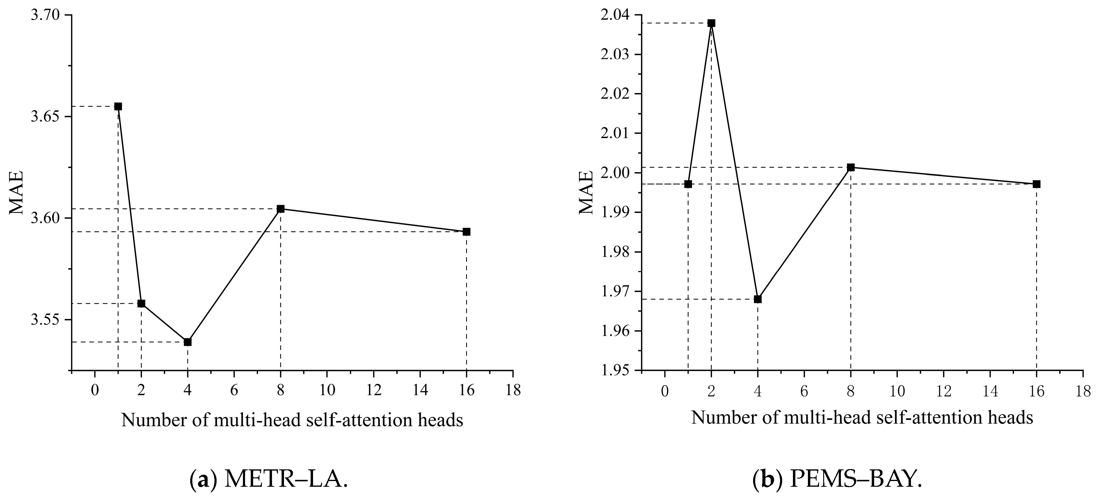
4.4.4. Parameter Sensitivity

The number of heads in the multi-head self-attention mechanism is also an important parameter, which controls how many heads the input feature map is divided into and computed in parallel. The selection of the number of heads can affect the effect of multi-head self-attention. Experiments were carried out on the datasets METR–LA and PEMS–BAY with the number of heads being 1, 2, 4, 8, and 16, and the results are shown in Figure 10.

Figure 10. Multi-head self-attention head number experiment.

It can be obtained from Figure 10 that both too many heads and too few heads have a great influence on the experimental results. When the number of heads is too large, too many heads will lead to low computational efficiency and prone to overfitting. When the number of heads is too small, too few heads will lead to insufficient representation power and prone to underfitting. Therefore, after comprehensively comparing the experimental results of the two datasets, the number of heads was set to 4 in both the METR–LA dataset and the PEMS–BAY dataset in this study.

4.5. Discussion

In the experimental comparison in Section 4.4, it can be observed that our proposed MSGSGCN significantly improves the accuracy of the model prediction. Compared to other baseline models, the MSGSGCN can effectively learn long-distance spatiotemporal information by capturing the spatiotemporal correlation between nodes. Furthermore, in the visualized fitting graph, it can be seen that our model does not deliberately fit the noise in the dataset. Additionally, the efficacy of the proposed module was verified through ablation experiments, and suitable parameter settings were determined via comparative testing. Overall, the MSGSGCN performs excellently in traffic data prediction performance. Figure 11 shows a visual representation of the accuracy improvement in the model compared to the baseline model.

Figure 11. Percentage reduction in error compared to the baseline model.

5. Conclusions

In this paper, we propose a multi-head self-attention gated spatiotemporal graph convolutional network. We construct a node correlation estimator using multi-head self-attention and linear transformations to learn the dynamic spatiotemporal correlations between nodes. Additionally, we design a novel spatiotemporal module to capture the complex spatiotemporal information of traffic data, effectively capturing long-term traffic patterns while ignoring irrelevant information. We validate the accuracy of our proposed model using the METR–LA and PEMS–BAY datasets, and our results show an average error reduction of 27.4% and 20.6%, respectively, compared to the eight baseline models. However, the MSGSGCN still has the following shortcomings:

• In terms of computational efficiency, the GGCF module requires a longer training time compared to the NCE module, and the accuracy improvement is not significant. This is mainly because each gating unit needs to train many learnable parameters, whereas the parameters for each spatiotemporal module layer are not shared.
• In terms of model generalizability, an adjacency matrix that describes the network structure still needs to be constructed before training, which limits the model’s versatility across different road networks.
• In terms of considering external factors, the model’s architecture does not sufficiently take into account other external influences that affect network data, such as weather and holidays, which leads to the model’s inability to simulate real-world traffic patterns accurately.

Therefore, in the future, we plan to explore the integration of additional external factor learning modules and adaptive modules to enhance the model’s generalizability and to utilize generic learnable parameters to reduce the model’s complexity, further boosting its practical applicability.

References

1. Duan, H.M.; Wang, G. Partial differential grey model based on control matrix and its application in short-term traffic flow prediction. Appl. Math. Model. 2023, 116, 763–785. [Google Scholar] [CrossRef]
2. Feng, A.; Tassiulas, L. Adaptive graph spatial-temporal transformer network for traffic forecasting. In Proceedings of the 31st ACM International Conference on Information & Knowledge Management, Atlanta, GA, USA, 17–21 October 2022; pp. 3933–3937. [Google Scholar]
3. Liu, H.T.; Wang, H.F. Real-time anomaly detection of network traffic based on CNN. Symmetry 2023, 15, 1205. [Google Scholar] [CrossRef]
4. Han, X.; Zhu, G.; Zhao, L.; Du, R.H.; Wang, Y.H.; Chen, Z.; Liu, Y.; He, S.L. Ollivier–Ricci curvature based spatio-temporal graph neural networks for traffic flow forecasting. Symmetry 2023, 15, 995. [Google Scholar] [CrossRef]
5. Xiao, J.; Zhou, Z. Research progress of RNN language model. In Proceedings of the 2020 IEEE International Conference on Artificial Intelligence and Computer Applications (ICAICA), Dalian, China, 27–29 June 2020; pp. 1285–1288. [Google Scholar]
6. Wang, Y.H.; Fang, S.; Zhang, C.X.; Xiang, S.M.; Pan, C.H. TVGCN: Time-variant graph convolutional network for traffic forecasting. Neurocomputing 2022, 471, 118–129. [Google Scholar] [CrossRef]
7. Jiang, W.W.; Luo, J.Y.; He, M.; Gu, W.X. Graph neural network for traffic forecasting: The research progress. ISPRS Int. J. Geo-Inf. 2023, 12, 100. [Google Scholar] [CrossRef]
8. Bui, K.H.N.; Cho, J.; Yi, H. Spatial-temporal graph neural network for traffic forecasting: An overview and open research issues. Appl. Intell. 2022, 52, 2763–2774. [Google Scholar] [CrossRef]
9. Ding, C.; Duan, J.X.; Zhang, Y.R.; Wu, X.K.; Yu, G.Z. Using an ARIMA-GARCH modeling approach to improve subway short-term ridership forecasting accounting for dynamic volatility. IEEE Trans. Intell. Transp. Syst. 2017, 19, 1054–1064. [Google Scholar] [CrossRef]
10. Mehdi, H.; Pooranian, Z.; Vinueza Naranjo, P.G.V. Cloud traffic prediction based on fuzzy ARIMA model with low dependence on historical data. Trans. Emerg. Telecommun. Technol. 2022, 33, e3731. [Google Scholar] [CrossRef]
11. Luo, X.; Peng, J.; Liang, J. Directed hypergraph attention network for traffic forecasting. IET Intell. Transp. Syst. 2022, 16, 85–98. [Google Scholar] [CrossRef]
12. Hou, Z.W.; Du, Z.X.; Yang, G.; Yang, Z. Short-term passenger flow prediction of urban rail transit based on a combined deep learning model. Appl. Sci. 2022, 12, 7597. [Google Scholar] [CrossRef]
13. Williams, B.M.; Hoel, L.A. Modeling and forecasting vehicular traffic flow as a seasonal ARIMA process: Theoretical basis and empirical results. J. Transp. Eng. 2003, 129, 664–672. [Google Scholar] [CrossRef]
14. Kumar, B.P.; Hariharan, K. Time series traffic flow prediction with hyper-parameter optimized ARIMA models for intelligent transportation system. J. Sci. Ind. Res. 2022, 81, 408–415. [Google Scholar]
15. Yao, E.Z.; Zhang, L.J.; Li, X.H.; Yun, X. Traffic forecasting of back servers based on ARIMA-LSTM-CF hybrid model. Int. J. Comput. Intell. Syst. 2023, 16, 65. [Google Scholar] [CrossRef]
16. Lohrasbinasab, I.; Shahraki, A.; Taherkordi, A.; Jurcut, A.D. From statistical-to machine learning-based network traffic prediction. Trans. Emerg. Telecommun. Technol. 2022, 33, e4394. [Google Scholar] [CrossRef]
17. Cai, P.L.; Wang, Y.P.; Lu, G.Q.; Chen, P.; Ding, C.; Sun, J.P. A spatiotemporal correlative k-nearest neighbor model for short-term traffic multistep forecasting. Transp. Res. Part C Emerg. Technol. 2016, 62, 21–34. [Google Scholar] [CrossRef]
18. Feng, X.X.; Ling, X.Y.; Zheng, H.F.; Chen, Z.H.; Xu, Y.W. Adaptive multi-kernel SVM with spatial–temporal correlation for short-term traffic flow prediction. IEEE Trans. Intell. Transp. Syst. 2018, 20, 2001–2013. [Google Scholar] [CrossRef]
19. Xie, P.; Li, T.R.; Liu, J.; Du, S.D.; Yang, X.; Zhang, J.B. Urban flow prediction from spatiotemporal data using machine learning: A survey. Inf. Fusion 2020, 59, 1–12. [Google Scholar] [CrossRef]
20. Razali, N.A.M.; Shamsaimon, N.; Ishak, K.K.; Ramli, S.; Amran, M.F.M.; Sukardi, S. Gap, techniques and evaluation: Traffic flow prediction using machine learning and deep learning. J. Big Data. 2021, 8, 152. [Google Scholar] [CrossRef]
21. Ai, D.H.; Jiang, G.Y.J.; Lam, S.K.; He, P.L.; Li, C.W. Computer vision framework for crack detection of civil infrastructure—A review. Eng. Appl. Artif. Intell. 2023, 117, 105478. [Google Scholar] [CrossRef]
22. Goyal, S.; Doddapaneni, S.; Khapra, M.M.; Ravindran, B. A survey of adversarial defenses and robustness in NLP. ACM Comput. Surv. 2023, 55, 1–39. [Google Scholar] [CrossRef]
23. Seshia, S.A.; Jha, S.; Dreossi, T. Semantic adversarial deep learning. IEEE Des. Test. 2020, 37, 8–18. [Google Scholar] [CrossRef]
24. Zhang, Y.; Qian, F.; Xiao, F. GS-RNN: A novel RNN optimization method based on vanishing gradient mitigation for HRRP sequence estimation and recognition. In Proceedings of the 2020 IEEE 3rd International Conference on Electronics Technology (ICET), Chengdu, China, 8–12 May 2020; pp. 840–844. [Google Scholar]
25. Tian, Y.; Zhang, K.L.; Li, J.Y.; Lin, X.X.; Yang, B.L. LSTM-based traffic flow prediction with missing data. Neurocomputing 2018, 318, 297–305. [Google Scholar] [CrossRef]
26. Kang, D.; Lv, Y.; Chen, Y. Short-term traffic flow prediction with LSTM recurrent neural network. In Proceedings of the 2017 IEEE 20th International Conference on Intelligent Transportation Systems (ITSC), Yokohama, Japan, 16–19 October 2017; pp. 1–6. [Google Scholar]
27. Abdullah, S.M.; Periyasamy, M.; Kamaludeen, N.A.; Towfek, S.K.; Marappan, R.; Raju, S.K.; Alharbi, A.H.; Khafaga, D.S. Optimizing traffic flow in smart cities: Soft GRU-based recurrent neural networks for enhanced congestion prediction using deep learning. Sustainability 2023, 15, 5949. [Google Scholar] [CrossRef]
28. Ma, C.X.; Zhao, Y.P.; Dai, G.W.; Xu, X.C.; Wong, S.C. A novel STFSA-CNN-GRU hybrid model for short-term traffic speed prediction. IEEE Trans. Intell. Transp. Syst. 2022, 24, 3728–3737. [Google Scholar] [CrossRef]
29. Bao, Y.X.; Shi, Q.; Shen, Q.Q.; Cao, Y. Spatial-temporal 3D residual correlation network for urban traffic status prediction. Symmetry 2021, 14, 33. [Google Scholar] [CrossRef]
30. Ni, Q.J.; Zhang, M. STGMN: A gated multi-graph convolutional network framework for traffic flow prediction. Appl. Intell. 2022, 52, 15026–15039. [Google Scholar] [CrossRef]
31. Bao, Y.X.; Liu, J.L.; Shen, Q.Q.; Cao, Y.; Ding, W.P.; Shi, Q. PKET-GCN: Prior knowledge enhanced time-varying graph convolution network for traffic flow prediction. Inf. Sci. 2023, 634, 359–381. [Google Scholar] [CrossRef]
32. Zhao, L.; Song, Y.J.; Zhang, C.; Liu, Y.; Wang, P.; Lin, T.; Deng, M.; Li, H.F. T-GCN: A temporal graph convolutional network for traffic prediction. IEEE Trans. Intell. Transp. Syst. 2019, 21, 3848–3858. [Google Scholar] [CrossRef]
33. Yu, B.; Yin, H.; Zhu, Z. Spatio-temporal graph convolutional networks: A deep learning framework for traffic forecasting. arXiv 2017, arXiv:1709.04875. [Google Scholar]
34. Guo, S.; Lin, Y.; Feng, N.; Song, C.; Wan, H. Attention based spatial-temporal graph convolutional networks for traffic flow forecasting. In Proceedings of the AAAI Conference on Artificial Intelligence, Honolulu, HI, USA, 27 January–1 February 2019; Volume 33, pp. 922–929. [Google Scholar]
35. Li, Y.G.; Yu, R.; Shahabi, C.; Liu, Y. Diffusion convolutional recurrent neural network: Data-driven traffic forecasting. arXiv 2017, arXiv:1707.01926. [Google Scholar]
36. Wu, Z.; Pan, S.; Long, G.; Jiang, J.; Zhang, C. Graph WaveNet for deep spatial-temporal graph modeling. arXiv 2019, arXiv:1906.00121. [Google Scholar]
37. Song, C.; Lin, Y.; Guo, S.; Wan, H. Spatial-temporal synchronous graph convolutional networks: A new framework for spatial-temporal network data forecasting. In Proceedings of the AAAI Conference on Artificial Intelligence, New York, NY, USA, 7–12 February 2020; Volume 34, pp. 914–921. [Google Scholar]
38. Ye, Y.Q.; Xiao, Y.; Zhou, Y.X.; Li, S.W.; Zang, Y.F.; Zhang, Y.X. Dynamic multi-graph neural network for traffic flow prediction incorporating traffic accidents. Expert Syst. Appl. 2023, 234, 121101. [Google Scholar] [CrossRef]
39. Hassanat, A.; Alkafaween, E.; Tarawneh, A.S.; Elmougy, S. Applications review of hassanat distance metric. In Proceedings of the International Conference on Emerging Trends in Computing and Engineering Applications (ETCEA), Karak, Jordan, 23–24 November 2022; pp. 1–6. [Google Scholar]
40. Shao, Z.; Zhang, Z.; Wei, W.; Wang, F.; Xu, Y.; Cao, X. Decoupled dynamic spatial-temporal graph neural network for traffic forecasting. arXiv 2022, arXiv:2206.09112. [Google Scholar] [CrossRef]
41. Ye, J.; Sun, L.; Du, B.; Fu, Y.; Xiong, H. Coupled layer-wise graph convolution for transportation demand prediction. In Proceedings of the AAAI Conference on Artificial Intelligence, Virtually, 2–9 February 2021; Volume 35, pp. 4617–4625. [Google Scholar]
42. Rad, A.C.; Lemnaru, C.; Munteanu, A. A comparative analysis between efficient attention mechanisms for traffic forecasting without structural priors. Sensors 2022, 22, 7457. [Google Scholar] [CrossRef]
43. Drakulic, D.; Andreoli, J.M. Structured time series prediction without structural prior. arXiv 2022, arXiv:2202.03539. [Google Scholar]
Disclaimer/Publisher’s Note: The statements, opinions and data contained in all publications are solely those of the individual author(s) and contributor(s) and not of MDPI and/or the editor(s). MDPI and/or the editor(s) disclaim responsibility for any injury to people or property resulting from any ideas, methods, instructions or products referred to in the content.
Article Metrics
Citations
Article Access Statistics
Multiple requests from the same IP address are counted as one view.