
Optimal Estimation of Reliability Parameters for Modified Frechet-Exponential Distribution Using Progressive Type-II Censored Samples with Mechanical and Medical Data

 , and
, and
Abstract
1. Introduction
2. Maximum-Likelihood Estimation
3. Asymptotic Confidence Intervals
4. Bootstrap Confidence Intervals
4.1. Percentile Bootstrap (Boot-p) Confidence Interval
- (1)
- Calculate the ML estimates of the parameters and , say, and .
- (2)
- Produce a Pro-II C sample with size m from the MFE distribution using and from the algorithm described in [22].
- (3)
- Calculate the ML estimates of the bootstrap sample, say, and .
- (4)
- Repeat steps 2 and 3 N times and obtain
- (5)
- Sort the bootstrap estimates to obtain an approximate distribution of and .
4.2. Bootstrap-t (Boot-t) Confidence Interval
- (1)
- Repeat steps (1)–(3) in Boot-p.
- (2)
- From the variance–covariance matrix (), we have the t-statistic of as =
- (3)
- Repeat steps 1 and 2 N times and obtain
- (4)
- Sort to obtain an approximate distribution of , , ,…,
5. Bayes Estimation
- (1)
- Begin with (, ) as an initial guess.
- (2)
- Put .
- (3)
- Generate and from and with the normal proposal distribution using the M-H approach shown below.
- (4)
- Generate a proposal from , var()) and a proposal from , var()).
- (i)
- Calculate the acceptance probabilities
- (ii)
- Produce , and from a uniform (0,1) distribution.
- (iii)
- If < , accept the suggestion and set = , else put = .
- (iv)
- If < , accept the suggestion and set = , else put = .
- (5)
- Calculate the survival and failure hazard functions and (t) by substituting and
- (6)
- Put .
- (7)
- Repeat Steps (3)–(6) N times to obtain , and
- (8)
- To calculate the CRs of and and ,as ; then, the CRIs of is
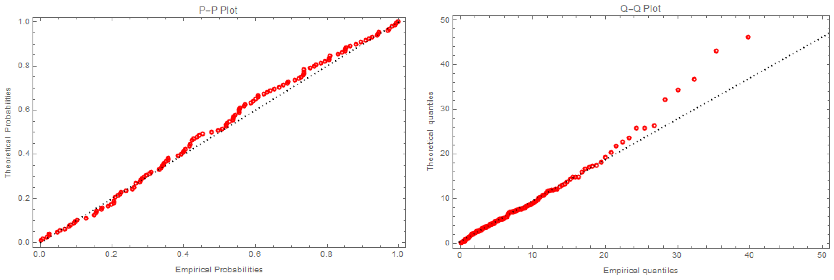
6. Applications
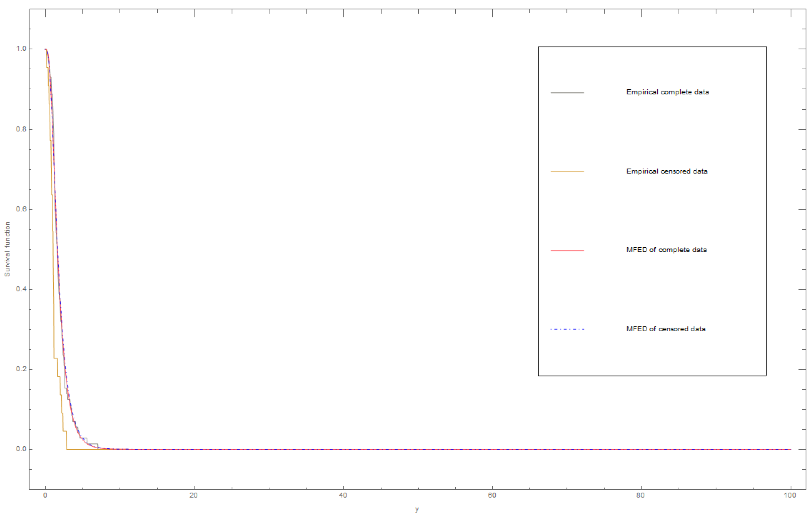
6.1. Dataset I
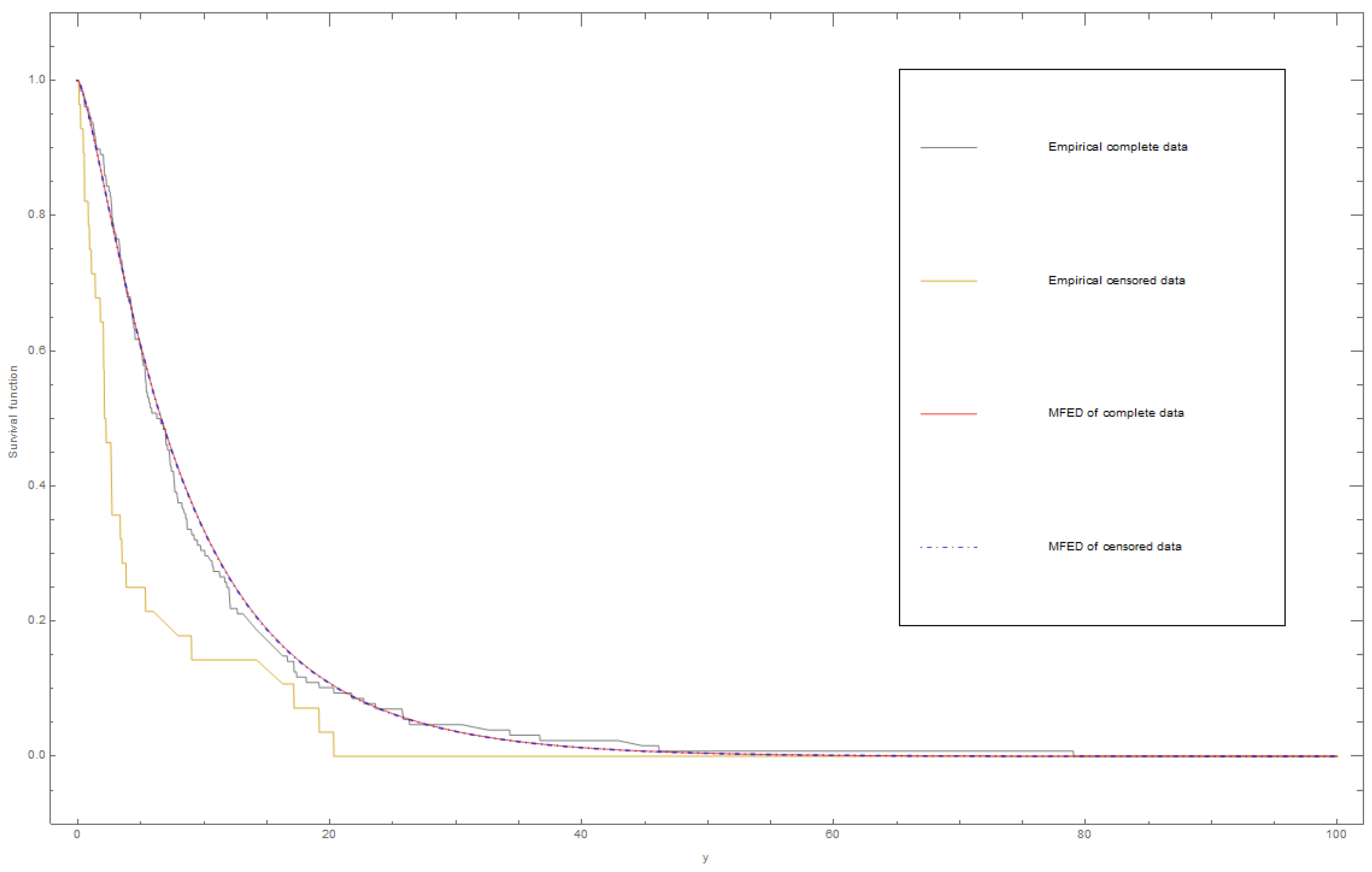
6.2. Dataset II
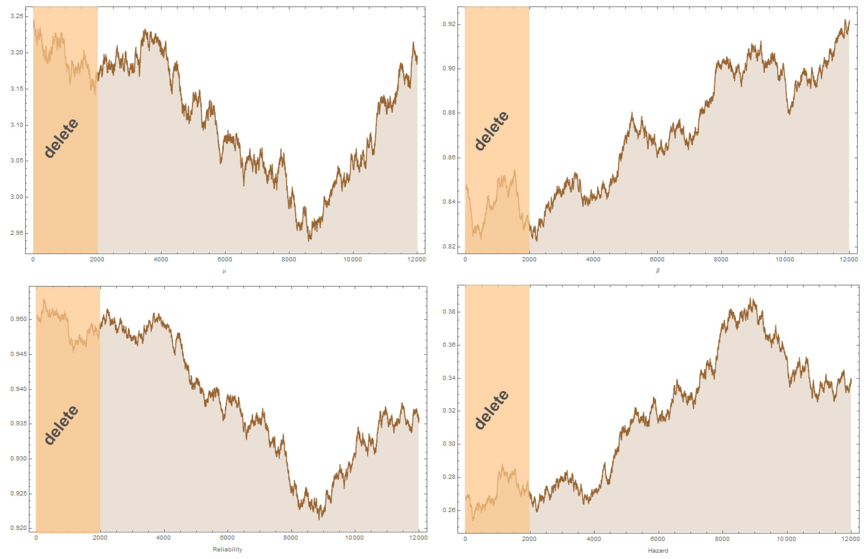
7. Simulation
8. Results and Discussion
9. Conclusions
Author Contributions
Funding
Data Availability Statement
Acknowledgments
Conflicts of Interest
Appendix A
- This code was executed using Wolfram Mathematica software, version 11.3, to find the parameters of the MFE distribution for progressive type-II censored sample.
- complete-data = {0.1, 0.33, 0.44, 0.56, 0.59, 0.72, 0.74, 0.77, 0.92, 0.93, 0.96, 1, 1, 1.02, 1.05, 1.07, 1.08, 1.08, 1.08, 1.09, 1.12, 1.13, 1.15, 1.16, 1.2, 1.21, 1.22, 1.22, 1.24, 1.3, 1.34, 1.36, 1.39, 1.44, 1.46, 1.53, 1.59, 1.6, 1.63, 1.63, 1.68, 1.71, 1.72, 1.76, 1.83, 1.95, 1.96, 1.97, 2.02, 2.13, 2.15, 2.16, 2.22, 2.3, 2.31, 2.4, 2.45, 2.51, 2.53, 2.54, 2.54, 2.78, 2.93, 3.27, 3.42, 3.47, 3.61, 4.02, 4.32, 4.58, 5.55, 7};
- x = {0.1, 0.33, 0.44, 0.56, 0.59, 0.72, 0.74, 0.77, 0.92, 0.93, 1, 1, 1.02, 1.05, 1.08, 1.08, 1.09, 1.59, 1.95, 2.13, 2.31, 2.78}
- n = Length[complete-data]; m = Length[x];
- R = {10, 0, 0, 0, 0, 0, 0, 0, 0, 0, 0, 10, 10, 10, 10, 0, 0, 0, 0, 0, 0, 0}
- L = Log[]
- ML = FindRoot[{ L == 0, L == 0 }, {{, 4}, {, 1}}];
- mu = /. ML;
- beta = /. ML;
- t = 0.5;
- Sur[ _, _ ] := Divide[(E^-1) - (E^-(1 - E^(-*t))^, (E^-1) - 1];
- Haz[_, _ ] := Divide[(**(E^((-*t) - (1 - E^(-*t))^))*((1 - E^(-*t))^(-1))), (E^-(1 - E^(-*t))^) - (E^-1)];
- S = Sur[mu, beta];
- H = Haz[mu, beta];
- {mu, beta, S, H}
References
- Klein, J.P.; Moeschberger, M.L. Survival Analysis: Techniques for Censored and Truncated Data; Springer: New York, NY, USA, 2003; Volume 1230. [Google Scholar]
- Albert, J. Bayesian Computation with R; Springer Science & Business Media: New York, NY, USA, 2009. [Google Scholar]
- Aggarwala, R.; Balakrishnan, N. Some properties of progressive censored order statistics from arbitrary and uniform distributions with applications to inference and simulation. J. Stat. Plan. Inference 1998, 70, 35–49. [Google Scholar] [CrossRef]
- Qin, X.; Yu, J.; Gui, W. Goodness-of-fit test for exponentiality based on spacings for general progressive Type-II censored data. J. Appl. Stat. 2022, 49, 599–620. [Google Scholar] [CrossRef] [PubMed]
- Bairamov, I.; Eryılmaz, S. Spacings, exceedances and concomitants in progressive type II censoring scheme. J. Stat. Plan. Inference 2006, 136, 527–536. [Google Scholar] [CrossRef]
- Montanari, G.C.; Mazzanti, G.; Cacciari, M.; Fothergill, J.C. Optimum estimators for the Weibull distribution from censored test. data. Progressively-censored tests [breakdown statistics]. IEEE Trans. Dielectr. Electr. Insul. 1998, 5, 157–164. [Google Scholar] [CrossRef]
- Tse, S.K.; Yang, C.; Yuen, H.K. Statistical analysis of Weibull distributed lifetime data under Type II progressive censoring with binomial removals. J. Appl. Stat. 2000, 27, 1033–1043. [Google Scholar] [CrossRef]
- Khalifa, E.H.; Ramadan, D.A.; Alqifari, H.N.; El-Desouky, B.S. Bayesian Inference for Inverse Power Exponentiated Pareto Distribution Using Progressive Type-II Censoring with Application to Flood-Level Data Analysis. Symmetry 2024, 16, 309. [Google Scholar] [CrossRef]
- Buzaridah, M.M.; Ramadan, D.A.; El-Desouky, B.S. Estimation of Some Lifetime Parameters of Flexible Reduced Logarithmic-Inverse Lomax Distribution under Progressive Type-II Censored Data. J. Math. 2022, 2022, 1690458. [Google Scholar] [CrossRef]
- Attwa, R.A.E.W.; Sadk, S.W.; Radwan, T. Estimation of Marshall–Olkin Extended Generalized Extreme Value Distribution Parameters under Progressive Type-II Censoring by Using a Genetic Algorithm. Symmetry 2024, 16, 669. [Google Scholar] [CrossRef]
- Chen, Q.; Gui, W. Statistical inference of the generalized inverted exponential distribution under joint progressively type-II censoring. Entropy 2022, 24, 576. [Google Scholar] [CrossRef] [PubMed]
- Hasaballah, M.M.; Tashkandy, Y.A.; Bakr, M.E.; Balogun, O.S.; Ramadan, D.A. Classical and Bayesian inference of inverted modified Lindley distribution based on progressive type-II censoring for modeling engineering data. AIP Adv. 2024, 14, 035021. [Google Scholar] [CrossRef]
- Ramadan, D.A.; Tashkandy, Y.A.; Bakr, M.E.; Balogun, O.S.; Hasaballah, M.M. Analysis of Marshall–Olkin extended Gumbel type-II distribution under progressive type-II censoring with applications. AIP Adv. 2024, 14, 055137. [Google Scholar] [CrossRef]
- Farhat, A.T.; Ramadan, D.A.; El-Desouky, B.S. Statistical Inference of Modified Frechet–Exponential Distribution with Applications to Real-Life Data. Appl. Math. Inf. Sci. 2023, 17, 109–124. [Google Scholar]
- Bjerkedal, T. Acquisition of Resistance in Guinea Pies infected with Different Doses of Virulent Tubercle Bacilli. Am. J. Hyg. 1960, 72, 130–148. [Google Scholar] [PubMed]
- Lee, E.T.; Wang, J. Statistical Methods for Survival Data Analysis; John Wiley & Sons: Hoboken, NJ, USA, 2003; Volume 476. [Google Scholar]
- Ahmed, E.A. Estimation of some lifetime parameters of generalized Gompertz distribution under progressively type-II censored data. Appl. Math. Model. 2015, 39, 5567–5578. [Google Scholar] [CrossRef]
- Lawless, J.F. Statistical Models and Methods for Lifetime Data; John Wiley & Sons: Hoboken, NJ, USA, 2011. [Google Scholar]
- Greene, W.H. Econometric Analysis, 4th ed.; Prentice Hall: New York, NY, USA, 2000. [Google Scholar]
- Efron, B. The Jackknife, the Bootstrap and Other Resampling Plans; Society for Industrial and Applied Mathematics: Philadelphia, PA, USA, 1982. [Google Scholar]
- Hall, P. Theoretical comparison of bootstrap confidence intervals. Ann. Stat. 1988, 16, 927–953. [Google Scholar] [CrossRef]
- Balakrishnan, N.; Sandhu, R.A. Best linear unbiased and maximum likelihood estimation for exponential distributions under general progressive type-II censored samples. SankhyĀ Indian J. Stat. Ser. 1996, 58, 1–9. [Google Scholar]
- Amir-Ahmadi, P.; Matthes, C.; Wang, M.C. Choosing prior hyperparameters: With applications to time-varying parameter models. J. Bus. Econ. Stat. 2020, 38, 124–136. [Google Scholar] [CrossRef]
- Akaike, H. A new look at the statistical model identification. IEEE Trans. Autom. Control. 1974, 19, 716–723. [Google Scholar] [CrossRef]


| Parameters | Goodness of Fit Test | ||||
|---|---|---|---|---|---|
| Schemes: (Ri, i = 1 … m) | Methods | k–s | p-Value | ||
| MLE | 3.48428 | 0.896263 | 0.0871889 | 0.648787 | |
| MLE | 3.06257 | 0.8476020 | 0.113089 | 0.319988 | |
| SEL | 3.07114 | 0.8684135 | 0.122289 | 0.235379 | |
| Boot-p | 3.24335 | 0.908057 | 0.120389 | 0.251329 | |
| Boot-t | 3.14956 | 0.883567 | 0.119889 | 0.255656 | |
| MLE | 3.27225 | 0.906285 | 0.115989 | 0.291295 | |
| SEL | 3.29635 | 0.939405 | 0.129189 | 0.183824 | |
| Boot-p | 3.72982 | 1.00879 | 0.113589 | 0.314907 | |
| Boot-t | 3.60715 | 0.981452 | 0.113789 | 0.31289 | |
| MLE | 3.35838 | 0.903693 | 0.104689 | 0.413581 | |
| SEL | 3.18246 | 0.942841 | 0.145089 | 0.0986067 | |
| Boot-p | 3.9897 | 1.05588 | 0.110022 | 0.352371 | |
| Boot-t | 3.84561 | 1.02493 | 0.109222 | 0.361161 | |
| MLE | 3.23618 | 0.8465 | 0.0914889 | 0.587746 | |
| SEL | 3.09777 | 0.876023 | 0.122689 | 0.23212 | |
| Boot-p | 3.30261 | 0.802031 | 0.107422 | 0.381449 | |
| Boot-t | 3.19696 | 0.778243 | 0.115522 | 0.295785 | |
| MLE | 3.33041 | 0.873958 | 0.0936889 | 0.556999 | |
| SEL | 3.26006 | 0.896745 | 0.112789 | 0.323063 | |
| Boot-p | 4.35966 | 1.1255 | 0.108922 | 0.364493 | |
| Boot-t | 4.20745 | 1.09441 | 0.107822 | 0.37688 | |
| Parameters | MLE | Boot-p | Boot-t | SEL | LINEX | ||
|---|---|---|---|---|---|---|---|
| 3.23618 | 3.09777 | 3.30261 | 3.19696 | 3.10375 | 3.09777 | 3.09173 | |
| 0.8465 | 0.876023 | 0.802031 | 0.778243 | 0.876673 | 0.876023 | 0.875369 | |
| S | 0.950235 | 0.937079 | 0.954676 | 0.953176 | 0.937149 | 0.937079 | 0.937009 |
| h | 0.267949 | 0.323856 | 0.235526 | 0.23778 | 0.32514 | 0.323856 | 0.322561 |
| Parameters | MLE | Boot-p | Boot-t | MCMC |
|---|---|---|---|---|
| Parameters | Goodness of Fit Test | ||||
|---|---|---|---|---|---|
| Schemes: (Ri, i = 1 … m) | Methods | k–s | p-Value | ||
| MLE | 1.37069 | 0.102992 | 0.0557625 | 0.826817 | |
| MLE | 1.33365 | 0.108417 | 0.061525 | 0.725065 | |
| SEL | 1.27695 | 0.111408 | 0.082525 | 0.355579 | |
| Boot-p | 1.03811 | 0.160333 | 0.279125 | 5.603 × | |
| Boot-t | 1.01957 | 0.155266 | 0.275625 | 9.153 × | |
| MLE | 1.31271 | 0.094352 | 0.0754625 | 0.467832 | |
| SEL | 1.22791 | 0.101671 | 0.078625 | 0.415338 | |
| Boot-p | 0.985561 | 0.133855 | 0.241825 | 7.612 × | |
| Boot-t | 0.96491 | 0.128156 | 0.237025 | 1.361 × | |
| MLE | 1.35442 | 0.0981315 | 0.0709625 | 0.547792 | |
| SEL | 1.25131 | 0.108465 | 0.084625 | 0.325827 | |
| Boot-p | 1.02624 | 0.149208 | 0.260125 | 7.467 × | |
| Boot-t | 1.0034 | 0.142394 | 0.254025 | 1.649 × | |
| MLE | 1.29638 | 0.0848472 | 0.112363 | 0.0822362 | |
| SEL | 1.22392 | 0.0899226 | 0.0692625 | 0.579239 | |
| Boot-p | 0.993563 | 0.132981 | 0.236525 | 1.445 × | |
| Boot-t | 0.975827 | 0.12803 | 0.232125 | 2.433 × | |
| MLE | 1.37207 | 0.103355 | 0.0546625 | 0.844499 | |
| SEL | 1.28927 | 0.110197 | 0.076825 | 0.444799 | |
| Boot-p | 1.0199 | 0.160209 | 0.285825 | 2.1524 × | |
| Boot-t | 1.00091 | 0.153881 | 0.280025 | 4.934 × | |
| Parameters | MLE | Boot-p | Boot-t | SEL | LINEX | ||
|---|---|---|---|---|---|---|---|
| 1.37207 | 1.28927 | 1.0199 | 1.00091 | 1.28975 | 1.28927 | 1.2888 | |
| 0.103355 | 0.110197 | 0.160209 | 0.153881 | 0.110198 | 0.110197 | 0.110196 | |
| S | 0.974008 | 0.963972 | 0.886242 | 0.885236 | 0.963976 | 0.963972 | 0.963967 |
| h | 0.0707634 | 0.092579 | 0.237686 | 0.235966 | 0.092598 | 0.092579 | 0.092561 |
| Parameters | MLE | Boot-p | Boot-t | MCMC |
|---|---|---|---|---|
| (0.898159, 1.84598) | (0.79254, 1.33923) | (0.77872, 1.31299) | (1.25177, 1.3291) | |
| (0.041874, 0.16483) | (0.10637, 0.21984) | (0.10158, 0.21984) | (0.10812, 0.11208) | |
| (0.95197, 0.99604) | (0.83778, 0.93014) | (0.83712, 0.92892) | (0.95989, 0.96778) | |
| (0.028886, 0.11264) | (0.16882, 0.30069) | (0.16907, 0.29706) | (0.08499, 0.10046) |
| MLE | ACIs | SEL | LINEX | MCMCs | ||||
|---|---|---|---|---|---|---|---|---|
| I | 2.16998 | 2.00604 | 2.17701 | 2.1774 | 2.17701 | 2.17662 | 0.060812 | |
| II | 2.02973 | 1.82165 | 2.03111 | 2.03142 | 2.03111 | 2.0308 | 0.054685 | |
| III | 2.23718 | 2.16815 | 2.23948 (0.453443) | 2.23995 (0.454169) | 2.23948 (0.453442) | 2.23902 (0.452716) | 0.065402 | |
| I | 1.97095 | 1.61069 | 1.97795 | 1.9782 | 1.97795 | 1.97769 | 0.049179 | |
| II | 2.25528 | 1.89352 | 2.26128 | 2.26163 | 2.26128 | 2.26092 | 0.057295 | |
| III | 2.17286 | 1.85062 | 2.17874 | 2.17907 | 2.17874 | 2.1784 | 0.055978 | |
| I | 2.58882 | 2.19919 | 2.59849 | 2.59896 | 2.59849 | 2.59802 | 0.067197 | |
| II | 2.30055 | 1.86829 | 2.30363 | 2.30396 | 2.30363 | 2.30331 | 0.056075 | |
| III | 2.16779 | 1.81472 | 2.17012 | 2.17042 | 2.17012 | 2.16981 | 0.054335 | |
| MLE | ACIs | SEL | LINEX | MCMCs | ||||
|---|---|---|---|---|---|---|---|---|
| I | 1.91449 | 1.62157 | 1.92162 | 1.92187 | 1.92162 | 1.92156 | 0.049912 | |
| II | 1.95801 | 1.83074 | 1.97175 | 1.9721 | 1.97175 | 1.97163 | 0.058505 | |
| III | 2.19592 | 2.05705 | 2.21727 (0.366692) | 2.21772 (0.36711) | 2.21727 (0.366692) | 2.21698 (0.366275) | 0.066751 | |
| I | 1.90966 | 1.45972 | 1.91717 | 1.91738 | 1.91717 | 1.91706 | 0.045267 | |
| II | 2.25065 | 1.71912 | 2.26215 | 2.26245 | 2.26215 | 2.2619 | 0.054304 | |
| III | 2.13511 | 1.6659 | 2.14886 | 2.14916 | 2.14886 | 2.14871 | 0.053743 | |
| I | 2.50456 | 1.75657 | 2.51274 | 2.51303 | 2.51274 | 2.51252 | 0.054106 | |
| II | 2.32928 | 1.79561 | 2.34341 | 2.34374 | 2.34341 | 2.34324 | 0.057476 | |
| III | 2.14467 | 1.72294 | 2.16252 | 2.16286 | 2.16252 | 2.16239 | 0.057432 | |
| MLE | ACIs | SEL | LINEX | MCMCs | ||||
|---|---|---|---|---|---|---|---|---|
| I | 0.296047 | 0.261184 | 0.29534 | 0.295359 | 0.29534 | 0.295344 | 0.013962 | |
| II | 0.268607 | 0.25623 | 0.265926 | 0.265945 | 0.265926 | 0.265914 | 0.014209 | |
| III | 0.243069 | 0.245318 | 0.239207 (0.004207) | 0.239227 (0.004207) | 0.239207 (0.004207) | 2.23919 (0.004207) | 0.014203 | |
| I | 0.272072 | 0.221083 | 0.271392 | 0.271405 | 0.271392 | 0.271388 | 0.011631 | |
| II | 0.232602 | 0.209662 | 0.231154 | 0.231167 | 0.231154 | 0.231148 | 0.011275 | |
| III | 0.247458 | 0.211584 | 0.245449 | 0.245462 | 0.245449 | 0.245441 | 0.011845 | |
| I | 0.215222 | 0.203304 | 0.214709 | 0.214719 | 0.214709 | 0.214702 | 0.010482 | |
| II | 0.222191 | 0.208613 | 0.220072 | 0.220084 | 0.220072 | 0.220068 | 0.011234 | |
| III | 0.245544 | 0.212217 | 0.242344 | 0.242359 | 0.242344 | 0.24234 | 0.012386 | |
| MLE | ACIs | SEL | LINEX | MCMCs | ||||
|---|---|---|---|---|---|---|---|---|
| I | 2.00856 | 1.55172 | 2.01515 | 2.01544 | 2.01515 | 2.0150 | 0.053796 | |
| II | 2.07285 | 1.74475 | 2.08691 | 2.08729 | 2.08691 | 2.08682 | 0.06135 | |
| III | 2.30192 | 1.96187 | 2.32382 (0.333662) | 2.32431 (0.334071) | 2.32382 (0.333662) | 2.32354 (0.333662) | 0.069322 | |
| I | 2.0285 | 1.38576 | 2.03539 | 2.03562 | 2.03539 | 2.03517 | 0.047439 | |
| II | 2.35371 | 1.64288 | 2.36494 | 2.36525 | 2.36494 | 2.36492 | 0.056113 | |
| III | 2.24246 | 1.58439 | 2.25605 | 2.25636 | 2.25605 | 2.25591 | 0.055758 | |
| I | 2.58837 | 1.6951 | 2.59596 | 2.59626 | 2.59596 | 2.59590 | 0.056071 | |
| II | 2.43065 | 1.7213 | 2.4448 | 2.44515 | 2.4448 | 2.4443 | 0.059131 | |
| III | 2.25318 | 1.63944 | 2.27134 | 2.2717 | 2.27134 | 2.27102 | 0.059463 | |
Disclaimer/Publisher’s Note: The statements, opinions and data contained in all publications are solely those of the individual author(s) and contributor(s) and not of MDPI and/or the editor(s). MDPI and/or the editor(s) disclaim responsibility for any injury to people or property resulting from any ideas, methods, instructions or products referred to in the content. |
© 2024 by the authors. Licensee MDPI, Basel, Switzerland. This article is an open access article distributed under the terms and conditions of the Creative Commons Attribution (CC BY) license (https://creativecommons.org/licenses/by/4.0/).
Share and Cite
Ramadan, D.A.; Farhat, A.T.; Bakr, M.E.; Balogun, O.S.; Hasaballah, M.M. Optimal Estimation of Reliability Parameters for Modified Frechet-Exponential Distribution Using Progressive Type-II Censored Samples with Mechanical and Medical Data. Symmetry 2024, 16, 1476. https://doi.org/10.3390/sym16111476
Ramadan DA, Farhat AT, Bakr ME, Balogun OS, Hasaballah MM. Optimal Estimation of Reliability Parameters for Modified Frechet-Exponential Distribution Using Progressive Type-II Censored Samples with Mechanical and Medical Data. Symmetry. 2024; 16(11):1476. https://doi.org/10.3390/sym16111476
Chicago/Turabian StyleRamadan, Dina A., Ahmed T. Farhat, M. E. Bakr, Oluwafemi Samson Balogun, and Mustafa M. Hasaballah. 2024. "Optimal Estimation of Reliability Parameters for Modified Frechet-Exponential Distribution Using Progressive Type-II Censored Samples with Mechanical and Medical Data" Symmetry 16, no. 11: 1476. https://doi.org/10.3390/sym16111476
APA StyleRamadan, D. A., Farhat, A. T., Bakr, M. E., Balogun, O. S., & Hasaballah, M. M. (2024). Optimal Estimation of Reliability Parameters for Modified Frechet-Exponential Distribution Using Progressive Type-II Censored Samples with Mechanical and Medical Data. Symmetry, 16(11), 1476. https://doi.org/10.3390/sym16111476