The Chen Autoregressive Moving Average Model for Modeling Asymmetric Positive Continuous Time Series

Abstract

In this paper, we introduce a new dynamic model for time series based on the Chen distribution, which is useful for modeling asymmetric, positive, continuous, and time-dependent data. The proposed Chen autoregressive moving average (CHARMA) model combines the flexibility of the Chen distribution with the use of covariates and lagged terms to model the conditional median response. We introduce the CHARMA structure and discuss conditional maximum likelihood estimation, hypothesis testing inference along with the estimator asymptotic properties of the estimator, diagnostic analysis, and forecasting. In particular, we provide closed-form expressions for the conditional score vector and the conditional information matrix. We conduct a Monte Carlo experiment to evaluate the introduced theory in finite sample sizes. Finally, we illustrate the usefulness of the proposed model by exploring two empirical applications in a wind-speed and maximum-temperature time-series dataset.

1. Introduction

Time series models have become increasingly popular for data analysis in various scientific fields. The widely recognized autoregressive moving average (ARMA) model [1] has been commonly employed for the modeling of univariate time series. However, this model may not always be suitable for all types of data. In many cases, real-world data do not adhere to the assumption of normality that is required for the estimation of ARMA model parameters [2]. Consequently, recent literature has introduced new non-Gaussian time-series models that assume different probability distributions.

A general time-series model, known as the generalized autoregressive moving average (GARMA), was proposed in [3] as an extension of generalized linear models [4], specifically designed for dependent variables belonging to the canonical exponential family. Building upon similar approaches, the authors of [5] developed dynamic models using the beta family distribution, while [6] introduced a dynamic class of models for double-bounded interval data following the Kumaraswamy distribution. The authors of [7] proposed a dynamic regression model based on the Conway–Maxwell–Poisson distribution, and [8] presented a new generalized autoregressive moving average model based on the Bernoulli geometric distribution. Other recent contributions in this field include [9,10]. As a comprehensive reference for non-Gaussian dynamic regression, see [11].

Although numerous time series models have been published in the literature, there remains a limited availability of models specifically designed to handle continuous, asymmetric, and non-negative data. Given these circumstances, this work proposes a dynamic model based on the Chen distribution [12]. This distribution is very flexible and has garnered attention from the scientific community, as evidenced in [13,14,15]. The Chen distribution, which is characterized by shape parameters $\delta ,\lambda >0$ and has support in the positive real numbers ${\mathbb{R}}^{+}$, is defined by its probability density function [12]:

$$f_C(y;\lambda ,\delta )=\delta \lambda y^{\lambda -1}exp\{\delta [1-exp\left(y^{\lambda }\right)]+y^{\lambda }\},y>0.$$

The corresponding cumulative and quantile functions are respectively expressed by:

$$F_C(y;\lambda ,\delta )=1-exp\left\{\delta [1-exp\left(y^{\lambda }\right)]\right\}$$

and

$$Q_C(\tau ;\lambda ,\delta )={\left\{log\left[1-\left(\frac{log(1-\tau )}{\delta }\right)\right]\right\}}^{\frac{1}{\lambda }},0<\tau <1.$$

The original formulation of the Chen distribution relies on the parameters $\delta$ and $\lambda$, which may not have direct interpretability. However, for the purpose of regression and/or time-series modeling, it is more convenient to directly model the mean or median parameter of the distribution. Mean-based regression models are commonly employed for the modeling of response variables, but when the variable of interest exhibits asymmetric behavior, the more robust alternative is to use a median-based approach. Hence, in this work, we introduce a median-based reparameterization of the Chen distribution, which will serve as the foundation for a new flexible dynamic regression model for positive continuous data.

In this context, we introduce a novel class of dynamic regression models known as the Chen autoregressive moving average (CHARMA) model, which has specifically been designed for the modeling of asymmetric, continuous, positive, and time-dependent data. The CHARMA model assumes that the conditional distribution of the variable of interest follows the reparameterized Chen distribution. To model the conditional median, we employ a dynamic structure that includes autoregressive and moving average terms, time-varying regressors, and a strictly monotonic and twice-differentiable link function. We utilize the conditional likelihood theory to perform parameter inference for the CHARMA model. Additionally, we introduce closed-form expressions to the conditional score vector and the conditional information matrix, thus enabling computationally efficient inferences to be drawn for the model parameters. Diagnostic analysis and forecasting tools are also discussed to assess the model’s performance and predictive capabilities. To illustrate the practical application of the proposed model, we conduct a time-series analysis of average wind speed data taken from Rio Grande City, Brazil, and a time series analysis of monthly maximum temperature data from Teresina City, Brazil. In both applications, we compare the CHARMA model with other competing models and demonstrate the suitability of our proposed model and theory through empirical results. Overall, our findings highlight the effectiveness of the CHARMA model in modeling asymmetric, continuous, positive, and time-dependent data. The comprehensive analysis and empirical results further validate the practical applicability of our proposed model and theory.

The paper unfolds as follows. Section 2 introduces a new median-based parameterization for the Chen distribution and the dynamical CHARMA model. The conditional likelihood inference is discussed in Section 3. Section 4 focuses on model selection criteria, diagnostics, and forecasting. Numerical results are discussed in Section 5, wherein Section 5.1 presents a Monte Carlo simulation study, and Section 5.2 and Section 5.3 explore empirical applications in monthly average wind speed data and monthly average maximum temperature data, respectively. Concluding remarks are given in Section 6. Finally, some analytical details are presented in Appendix A.

2. The Proposed Model

Let $q\left(\tau \right)=q_{\tau }=Q_C(\tau ;\lambda ,\delta )$ represent the $\tau$th quantile of the Chen distribution, and $\delta$ can be expressed as $\delta =\frac{log(1-\tau )}{1-exp\left(q_{\tau }^{\lambda }\right)}$. The probability density function and cumulative distribution function of a Chen-distributed variable Y expressed in terms of its quantile-based parameterization can be given, respectively, by:

$$f(y;\lambda ,q_{\tau })=\frac{log(1-\tau )}{1-exp\left(q_{\tau }^{\lambda }\right)}\lambda y^{\lambda -1}exp\left\{\frac{log(1-\tau )}{1-exp\left(q_{\tau }^{\lambda }\right)}[1-exp\left(y^{\lambda }\right)]+y^{\lambda }\right\},y,q_{\tau }>0,$$

(1)

and

$$F(y;\lambda ,q_{\tau })=1-exp\left\{\frac{log(1-\tau )}{1-exp\left(q_{\tau }^{\lambda }\right)}[1-exp\left(y^{\lambda }\right)]\right\},y>0.$$

Note that if we set $\tau =0.5$, the value of $q_{\tau }$ will correspond to the median ($\mu$) of variable Y, that is, $\mu =q_{0.5}$. Figure 1 illustrates different shapes of the Chen density of the reparameterized distribution, considering various values for $\lambda$ and $\mu$.

Figure 1. The probability density function of the reparameterized Chen distribution with different parameter values.

Let ${\left\{Y_t\right\}}_{t\in \mathbb{Z}}$ be a stochastic process, where each $Y_t$—conditioned on the previous information set ${\mathcal{F}}_{t-1}$ consisting of observations up to time $t-1$—follows a Chen distribution, as defined in (1), with $\tau =0.5$. Using the median-based parameterization, the conditional density function of $Y_t$ is given by:

$$f(y_t;\lambda ,{\mu }_t|{\mathcal{F}}_{t-1})=\frac{log\left(0.5\right)}{1-exp\left({\mu }_t^{\lambda }\right)}\lambda y_t^{\lambda -1}exp\left\{\frac{log\left(0.5\right)}{1-exp\left({\mu }_t^{\lambda }\right)}[1-exp\left(y_t^{\lambda }\right)]+y_t^{\lambda }\right\},y_t>0,$$

(2)

where ${\mu }_t$ is the conditional median of $Y_t$, and the parameter $\lambda$ is considered fixed for all $t\in \mathbb{Z}$. The dynamical structure of the proposed CHARMA ($p,q$) model is written as follows:

$${\eta }_t=g\left({\mu }_t\right)={\beta }_0+{\mathit{x}}_t^{\top }\mathit{\beta }+\sum _{j=1}^p{\varphi }_j[g\left(y_{t-j}\right)-{\mathit{x}}_{t-j}^{\top }\mathit{\beta }]+\sum _{j=1}^q{\theta }_j{r}_{t-j},$$

(3)

where ${\eta }_t$ represents the linear predictor, ${\beta }_0$ is an intercept, $\mathit{\beta }={({\beta }_1,\dots ,{\beta }_k)}^{\top }$ is an unknown k-dimensional parameter vector associated with exogenous covariates, ${\mathit{x}}_t={(x_{t1},\dots ,x_{tk})}^{\top }$ is the k-dimensional vector of explanatory covariates at time t, $\mathit{\varphi }={({\varphi }_1,\dots ,{\varphi }_p)}^{\top }$ and $\mathit{\theta }={({\theta }_1,\dots ,{\theta }_q)}^{\top }$ are the vectors of autoregressive and moving average parameters, respectively, and $g(·)$ is a strictly monotonic and twice-differentiable link function, where $g:{\mathbb{R}}^{+}\to \mathbb{R}$. In this study, the errors were considered as $r_t=g\left(y_t\right)-g\left({\mu }_t\right)$ on the predictor scale, following the approach of [6]. Due to the parametric space of ${\mu }_t$, we chose to use the logarithm as the link function because it provides non-negative values for ${\mu }_t=g^{-1}\left({\eta }_t\right)$ regardless of the values assigned to ${\eta }_t$. The proposed CHARMA ($p,q$) model is defined by (2) and (3), where p and q represent the dimensions of $\mathit{\varphi }$ and $\mathit{\theta }$, respectively, indicating the order of the ARMA dynamic component.

3. Conditional Likelihood Inference

The inference for the parameters of the CHARMA model can be made using the conditional maximum likelihood method, where the conditional maximum likelihood estimators (CMLE) are obtained by maximizing the logarithm of the conditional likelihood function. Let $y_1,\dots ,y_n$ be a sample from the CHARMA ($p,q$) model, and $\mathit{\gamma }={({\beta }_0,{\mathit{\beta }}^{\top },{\mathit{\varphi }}^{\top },{\mathit{\theta }}^{\top },\lambda )}^{\top }$ be the $(k+p+q+2)$-dimensional vector of the parameters. With the conditioning on the $m=max(p,q)$ first observations, the conditional log-likelihood function is given by:

$$\ell \left(\mathit{\gamma }\right)=\sum _{t=m+1}^n{\ell }_t({\mu }_t,\lambda ),$$

(4)

where

$$\begin{array}{cc}\hfill {\ell }_t({\mu }_t,\lambda )=& log\left[{\displaystyle \frac{log\left(0.5\right)}{1-exp\left({\mu }_t^{\lambda }\right)}}\right]+(\lambda -1)log\left(y_t\right)+log\left(\lambda \right)+{\displaystyle \frac{log\left(0.5\right)\left[1-exp\left(y_t^{\lambda }\right)\right]}{1-exp\left({\mu }_t^{\lambda }\right)}}+y_t^{\lambda }.\hfill \end{array}$$

3.1. Conditional Score Vector

The components of the conditional score vector $\mathit{U}\left(\mathit{\gamma }\right)=(U_{{\beta }_0}\left(\mathit{\gamma }\right),{\mathit{U}}_{\mathit{\beta }}{\left(\mathit{\gamma }\right)}^{\top },{\mathit{U}}_{\mathit{\varphi }}{\left(\mathit{\gamma }\right)}^{\top },$ ${\mathit{U}}_{\mathit{\theta }}{\left(\mathit{\gamma }\right)}^{\top },U_{\lambda }{\left(\mathit{\gamma }\right))}^{\top }$ are defined by the first derivatives of the conditional log-likelihood function with respect to each element of the parameter vector $\mathit{\gamma }$. Computing the derivatives of the function in (4) with respect to the i-th element of $\mathit{\gamma }$, ${\gamma }_i\ne \lambda$, for $i=1,\cdots ,(k+p+q+1)$, we obtain the following:

$$U_{{\gamma }_i}\left(\mathit{\gamma }\right)={\displaystyle \frac{\partial \ell \left(\mathit{\gamma }\right)}{\partial {\gamma }_i}}=\sum _{t=m+1}^n{\displaystyle \frac{\partial {\ell }_t({\mu }_t,\lambda )}{\partial {\mu }_t}}{\displaystyle \frac{d{\mu }_t}{d{\eta }_t}}{\displaystyle \frac{\partial {\eta }_t}{\partial {\gamma }_i}}.$$

Note that as ${\eta }_t=g\left({\mu }_t\right)$, we have $d{\mu }_t/d{\eta }_t=1/g^{\prime }\left({\mu }_t\right)$. Moreover, the derivative of ${\ell }_t({\mu }_t,\lambda )$ with respect to ${\mu }_t$ is given by:

$$v_t≔\frac{\partial {\ell }_t({\mu }_t,\lambda )}{\partial {\mu }_t}={\displaystyle \frac{\lambda exp\left({\mu }_t^{\lambda }\right){\mu }_t^{\lambda -1}}{1-exp\left({\mu }_t^{\lambda }\right)}}+{\displaystyle \frac{\lambda log\left(0.5\right)exp\left({\mu }_t^{\lambda }\right){\mu }_t^{\lambda -1}[1-exp\left(y_t^{\lambda }\right)]}{{[1-exp\left({\mu }_t^{\lambda }\right)]}^2}}.$$

The partial derivatives of ${\eta }_t$ with respect to the unknown parameters are computed recursively as follows:

$$\begin{array}{cc}\hfill \frac{\partial {\eta }_t}{\partial {\beta }_0}& =1-\sum _{j=1}^q{\theta }_j\frac{\partial {\eta }_{t-j}}{\partial {\beta }_0},\hfill \\ \hfill \frac{\partial {\eta }_t}{\partial {\beta }_i}& =x_{ti}-\sum _{j=1}^p{\varphi }_j{x}_{(t-j)i}-\sum _{j=1}^q{\theta }_j\frac{\partial {\eta }_{t-j}}{\partial {\beta }_i},i=1,\dots ,k,\hfill \\ \hfill \frac{\partial {\eta }_t}{\partial {\varphi }_i}& =g\left(y_{t-i}\right)-{\mathit{x}}_{t-i}^{\top }\mathit{\beta }-\sum _{j=1}^q{\theta }_j\frac{\partial {\eta }_{t-j}}{\partial {\varphi }_i},i=1,\dots ,p,\hfill \\ \hfill \frac{\partial {\eta }_t}{\partial {\theta }_i}& =g\left(y_{t-i}\right)-{\eta }_{t-i}-\sum _{j=1}^q{\theta }_j\frac{\partial {\eta }_{t-j}}{\partial {\theta }_i},i=1,\dots ,q.\hfill \end{array}$$

Finally, the derivative of ${\ell }_t({\mu }_t,\lambda )$ with respect to $\lambda$ is given by the following equation:

$$\begin{array}{cc}\hfill c_t≔{\displaystyle \frac{\partial {\ell }_t({\mu }_t,\lambda )}{\partial \lambda }}=& {\displaystyle \frac{{\mu }_t^{\lambda }exp\left({\mu }_t^{\lambda }\right)log\left({\mu }_t\right)}{1-exp\left({\mu }_t^{\lambda }\right)}}+{\displaystyle \frac{1}{\lambda }}+{\displaystyle \frac{log\left(0.5\right)exp\left({\mu }_t^{\lambda }\right){\mu }_t^{\lambda }log\left({\mu }_t\right)[1-exp\left(y_t^{\lambda }\right)]}{{[1-exp\left({\mu }_t^{\lambda }\right)]}^2}}\hfill \\ \hfill & +log\left(y_t\right)-{\displaystyle \frac{log\left(0.5\right)exp\left(y_t^{\lambda }\right)y_t^{\lambda }log\left(y_t\right)}{1-exp\left({\mu }_t^{\lambda }\right)}}+y_t^{\lambda }log\left(y_t\right).\hfill \end{array}$$

Then, the components of the conditional score vector can be written in matrix form as follows:

$$\begin{array}{cc}\hfill U_{{\beta }_0}\left(\mathit{\gamma }\right)& ={\mathit{a}}^{\top }\mathit{T}\mathit{v},\hfill \\ \hfill {\mathit{U}}_{\mathit{\beta }}\left(\mathit{\gamma }\right)& ={\mathit{M}}^{\top }\mathit{T}\mathit{v},\hfill \\ \hfill {\mathit{U}}_{\mathit{\varphi }}\left(\mathit{\gamma }\right)& ={\mathit{P}}^{\top }\mathit{T}\mathit{v},\hfill \\ \hfill {\mathit{U}}_{\mathit{\theta }}\left(\mathit{\gamma }\right)& ={\mathit{Q}}^{\top }\mathit{T}\mathit{v},\hfill \\ \hfill U_{\lambda }\left(\mathit{\gamma }\right)& ={\mathit{c}}^{\top }\mathbf{1},\hfill \end{array}$$

where $\mathit{v}={\left(v_{m+1},\dots ,v_n\right)}^{\top }$, $\mathit{T}=\mathrm{diag}\left\{\frac{1}{g^{\prime }\left({\mu }_{m+1}\right)},\dots ,\frac{1}{g^{\prime }\left({\mu }_n\right)}\right\}$, $\mathit{a}={\left(\frac{\partial {\eta }_{m+1}}{\partial {\beta }_0},\dots ,\frac{\partial {\eta }_n}{\partial {\beta }_0}\right)}^{\top }$, $\mathit{c}={\left(c_{m+1},\dots ,c_n\right)}^{\top }$, $\mathbf{1}$ is an $(n-m)$-dimensional vector of ones, and $\mathit{M},\mathit{P},\mathit{Q}$ are matrices with dimensions $(n-m)\times k,(n-m)\times p,\mathrm{and}(n-m)\times q$, respectively, whose $(i,j)\text{-}\mathrm{th}$ elements are given by the following equation:

$$M_{i,j}=\frac{\partial {\eta }_{i+m}}{\partial {\beta }_j},P_{i,j}=\frac{\partial {\eta }_{i+m}}{\partial {\varphi }_j},\mathrm{and}{Q}_{i,j}=\frac{\partial {\eta }_{i+m}}{\partial {\theta }_j}.$$

The CMLE of $\mathit{\gamma }$, denoted as $\widehat{\mathit{\gamma }}={({\widehat{\beta }}_0,{\widehat{\mathit{\beta }}}^{\top },{\widehat{\mathit{\varphi }}}^{\top },{\widehat{\mathit{\theta }}}^{\top },\widehat{\lambda })}^{\top }$, is obtained by solving the system $\mathit{U}\left(\mathit{\gamma }\right)=\mathbf{0}$, where $\mathbf{0}$ represents the null vector in ${\mathbb{R}}^{k+p+q+2}$. However, this system cannot be solved analytically, and iterative numerical methods must be employed to obtain an approximate solution. In such case, we utilize the Broyden–Fletcher–Goldfarb–Shanno (BFGS) method [16] with analytical derivatives.

3.2. Confidence Intervals and Hypothesis Testing

Inference for the confidence intervals and hypothesis testing parameters of the CHARMA model can be drawn using the asymptotic theory related to the CMLE. Under some mild mathematical regularity conditions, we have the following equation:

$$\widehat{\gamma }\stackrel{d}{\to }{\mathbf{N}}_{(k+p+q+2)}\left(\gamma ,{\mathit{J}}^{-1}\left(\gamma \right)\right),$$

(5)

where $\stackrel{d}{\to }$ denotes a convergence in distribution and ${\mathbf{N}}_{(k+p+q+2)}$ denotes the $(k+p+q+2)$-dimensional normal distribution, with a mean $\mathit{\gamma }$ and a variance–covariance matrix ${\mathit{J}}^{-1}\left(\mathit{\gamma }\right)$. The derivations and a closed-form expression for the joint observed information matrix $\mathit{J}\left(\mathit{\gamma }\right)$ for $\mathit{\gamma }$ are presented in Appendix A. In order to obtain the proof for these asymptotic results, we need to check if conditions 2.1–2.5 from [17] are fulfilled. Following closely related arguments, as in [6] for CMLE in the KARMA model and in [18] for the partial likelihood inference for time series following generalized linear modes, it is possible to guarantee these regularity conditions for the CHARMA model.

In hypothesis testing, we consider the interest in testing $H_0:{\gamma }_i={\gamma }_i^0$ versus $H_1:{\gamma }_i\ne {\gamma }_i^0$, where ${\gamma }_i^0$ is a specific value for the unknown parameter ${\gamma }_i$. Let ${\gamma }_i,i=1,2,\dots ,k+p+q+2$, the i-th element of the parameter vector $\mathit{\gamma }$. Based on approximation (5),

$$\begin{array}{c}\hfill \frac{({\widehat{\gamma }}_j-{\gamma }_j)}{\widehat{\mathrm{s}\mathrm{e}}\left({\widehat{\gamma }}_i\right)}\sim \mathcal{N}(0,1)\end{array}$$

holds for a large n, where ${\widehat{\gamma }}_i$ is the estimator of ${\gamma }_i$, $\widehat{\mathrm{s}\mathrm{e}}\left({\widehat{\gamma }}_i\right)=\sqrt{J^{ii}}$ is the asymptotic standard error of ${\widehat{\gamma }}_i$, and $J^{ii}$ is the i-th element of the diagonal of ${\mathit{J}}^{-1}\left(\widehat{\mathit{\gamma }}\right)$. The test statistic used in this context is the square root of Wald’s statistic, which can be expressed as follows:

$$\begin{array}{c}\hfill z=\frac{{\widehat{\gamma }}_i-{\gamma }_i^0}{\widehat{\mathrm{s}\mathrm{e}}\left({\widehat{\gamma }}_i\right)}.\end{array}$$

Under $H_0$ and in large sample sizes, z has an approximately standard normal distribution. The null hypothesis is rejected for values of $\left|z\right|$ higher than the upper quantile $\alpha /2$ of the standard normal distribution.

The asymptotic normality of the CMLE provides the means to construct confidence intervals. The asymptotic confidence interval of $100(1-\alpha )\%$ for each parameter ${\gamma }_i$ is given by:

$$\begin{array}{c}\hfill \left[{\widehat{\gamma }}_i\pm z_{\alpha /2}\widehat{\mathrm{s}\mathrm{e}}\left({\widehat{\gamma }}_i\right)\right],i=1,\dots ,k+p+q+2,\end{array}$$

where $z_{\alpha /2}$ is the upper quantile $\alpha /2$ of the standard normal distribution.

4. Model Selection, Diagnosis, and Prediction

In this section, we introduce several diagnostic measures for the assessment of the adequacy and goodness-of-fit of the proposed model. For model selection, we recommend utilizing the Akaike Information Criterion (AIC) [19] and the Bayesian Information Criterion (BIC). From among various competing fitted models, the preferred model is the one with the lowest AIC and BIC value.

Residual analysis is important for assessing the goodness-of-fit of a statistical model [11]. In this study, we consider the quantile residual, which is defined as follows [20]:

$$\begin{array}{c}\hfill r_t^{\left(q\right)}={\mathsf{\Phi }}^{-1}\left(F(y_t;\widehat{\lambda },{\widehat{\mu }}_t)\right),\end{array}$$

where $\mathsf{\Phi }(·)$ is the standard normal cumulative distribution function. If the model is well-fitted, $r_t^{\left(q\right)}$ is approximated distributed as a standard normal distribution, independently of the distribution of the response variable. These residuals are also expected to be independent, with a zero mean and a constant variance [1,21]. To evaluate the assumption that residuals are not auto-correlated, we suggest using the Ljung-Box test [22]. This test is conducted under the null hypothesis that the first auto-correlations of the residuals are zero.

A fitted model that successfully passes all diagnostic checks can be utilized for both in-sample and out-of-sample predictions. Predictions for the conditional median of the CHARMA$(p,q)$ model can be carried out by considering the estimation of ${\widehat{\mu }}_{m+1},\dots ,{\widehat{\mu }}_n$, replacing $\mathit{\gamma }$ with $\widehat{\mathit{\gamma }}$ in (3). Thus, the in-sample predictions, starting at $t=m+1$, are calculated as follows:

$$\begin{array}{c}\hfill {\widehat{\mu }}_t=g^{-1}\left({\widehat{\beta }}_0+{\mathit{x}}_t^{\top }\widehat{\mathit{\beta }}+\sum _{i=1}^p{\widehat{\varphi }}_i\left[g\left(y_{t-i}\right)-{\mathit{x}}_{t-i}^{\top }\widehat{\mathit{\beta }}\right]+\sum _{j=1}^q{\widehat{\theta }}_j{\widehat{r}}_{t-j}\right),\end{array}$$

where ${\widehat{r}}_t=g\left(y_t\right)-g\left({\widehat{\mu }}_t\right)$. For predictions h steps ahead, with $h\in \mathbb{N}$, the forecasts are calculated by the following equation:

$$\begin{array}{c}\hfill {\widehat{\mu }}_{n+h}=g^{-1}\left({\widehat{\beta }}_0+{\mathit{x}}_{n+h}^{\top }\widehat{\mathit{\beta }}+\sum _{i=1}^p\widehat{{\varphi }_i}\left[g^{*}\left(y_{n+h-i}\right)-{\mathit{x}}_{n+h-i}^{\top }\widehat{\mathit{\beta }}\right]+\sum _{j=1}^q\widehat{{\theta }_j}{\widehat{r}}_{n+h-j}\right),\end{array}$$

where ${\widehat{r}}_{n+h}=0$, $\forall h$, and

$$\begin{array}{c}\hfill g^{*}\left(y_t\right)=\left\{\begin{array}{cc}\hfill g\left({\widehat{\mu }}_t\right),& \mathrm{if}t>n,\\ \hfill g\left(y_t\right),& \mathrm{if}t\le n.\end{array}\right.\end{array}$$

To assess the quality of both in-sample and out-of-sample predictions, some accuracy measures can be employed. For this purpose, we recommend utilizing the mean absolute percentage error (MAPE) and mean squared error (MSE) as figures-of-merit to quantify the differences between the predicted values from the fitted model and the observed values. These measures are commonly used when comparing competing models [23,24,25].

5. Numerical Results

In this section, we aim to evaluate the CMLE of the CHARMA model parameters through the use of a Monte Carlo simulation study. Additionally, we will assess the performance of the proposed model in two empirical applications. Section 5.1 is focused on a simulated time series, while in Section 5.2 and Section 5.3, the numerical results based on two real datasets are presented. The R language [26] implementations used to fit the CHARMA model are available in https://github.com/RenataStone/CHARMA.git (accessed on 1 July 2023).

5.1. Monte Carlo Simulation

The Monte Carlo simulation study is presented to evaluate some of the CMLE properties of the proposed model parameters. The computational implementation was developed in the R language [26]. The number of Monte Carlo replications was set at 5000, and the sample sizes considered were $n=100,250,500$. We evaluate the mean, the percentage relative bias (RB%), defined as $\{E\left(\widehat{{\gamma }_i}\right)-{\gamma }_i\}/{\gamma }_i$, and the mean squared error (MSE) of the estimators.

In the simulation results, it was expected that as the sample size increased: (i) the mean of the estimates would be closer to the fixed parameter value, indicating that the estimators are asymptotically unbiased, and (ii) the MSE would be closer to zero, evidencing the consistency of the estimators. Table 1 presents the results of the Monte Carlo simulation in evaluating the CMLE introduced in Section 3 for three different scenarios: CHARMA$(1,0)$, CHARMA$(0,1)$, and CHARMA$(1,1)$. The parameter values considered in each scenario are also shown in Table 1. It is worth noting that even in the smallest simulated sample size ($n=100$), we observed good performance for the CMLE. As the sample size increased, the MSE value approached zero, thus providing numerical evidence for estimator consistency. Therefore, the simulation results bring evidence in favor of the introduced theory, the asymptotic properties of CMLE, and the computational implementations, which would allow for further empirical applications.

Table 1. Monte Carlo simulation results based on different orders of the CHARMA model with different sample sizes.

Scenarios	n	Parameter	Mean	RB%	MSE
CHARMA$(1,0)$		${\beta }_0=0.20$	$0.196$	$-1.840$	$0.011$
	100	${\varphi }_1=0.30$	$0.293$	$-2.248$	$0.005$
		$\lambda =0.70$	$0.711$	$1.546$	$0.002$
		${\beta }_0=0.20$	$0.201$	$0.335$	$0.004$
	250	${\varphi }_1=0.30$	$0.298$	$-0.644$	$0.002$
		$\lambda =0.70$	$0.705$	$0.688$	$0.001$
		${\beta }_0=0.20$	$0.200$	$0.187$	$0.002$
	500	${\varphi }_1=0.30$	$0.299$	$-0.195$	$0.001$
		$\lambda =0.70$	$0.703$	$0.373$	$0.000$
CHARMA$(0,1)$		${\beta }_0=0.20$	$0.197$	$-1.687$	$0.015$
	100	${\theta }_1=0.20$	$0.202$	$1.051$	$0.006$
		$\lambda =0.70$	$0.712$	$1.777$	$0.002$
		${\beta }_0=0.20$	$0.199$	$-0.309$	$0.006$
	250	${\theta }_1=0.20$	$0.201$	$0.655$	$0.002$
		$\lambda =0.70$	$0.705$	$0.699$	$0.001$
		${\beta }_0=0.20$	$0.200$	$-0.233$	$0.003$
	500	${\theta }_1=0.20$	$0.200$	$-0.169$	$0.001$
		$\lambda =0.70$	$0.703$	$0.362$	$0.000$
CHARMA$(1,1)$	100	${\beta }_0=0.30$	$0.298$	$-0.573$	$0.019$
		${\varphi }_1=0.20$	$0.201$	$0.477$	$0.022$
		${\theta }_1=0.30$	$0.295$	$-1.549$	$0.022$
		$\lambda =0.70$	$0.714$	$2.058$	$0.002$
	250	${\beta }_0=0.30$	$0.298$	$-0.821$	$0.007$
		${\varphi }_1=0.20$	$0.200$	$-0.062$	$0.009$
		${\theta }_1=0.30$	$0.300$	$-0.088$	$0.008$
		$\lambda =0.70$	$0.705$	$0.739$	$0.001$
	500	${\beta }_0=0.30$	$0.300$	$0.075$	$0.004$
		${\varphi }_1=0.20$	$0.202$	$0.977$	$0.004$
		${\theta }_1=0.30$	$0.298$	$-0.739$	$0.004$
		$\lambda =0.70$	$0.703$	$0.428$	$0.000$

5.2. Application to Monthly Average Wind-Speed Time Series in the City of Rio Grande

Wind speed is an important variable in climate studies involving economic factors, such as in applications associated with wind energy. Wind energy is considered to be one of the most mature renewable energy technologies and has experienced rapid growth in the past decade. It stands out in the planning carried out by national governments, who aim to diversify their renewable energy resources while minimizing environmental impact [27,28]. Despite the importance of studies on wind speed, a significant limitation observed in the literature is that most statistical studies that analyzed this variable did not account for the dependence between the observations in the time series. Therefore, the proposed model is suitable for wind-speed modeling, given that the support provided by the data is the set of positive real values and that the proposed CHARMA model considers the temporal dependence structure of this type of dataset.

In Brazil, one of the places considered to have the greatest wind energy potential is the country’s southern region. To illustrate the applicability of the proposed model, we developed an application for wind-speed data from a city in Rio Grande do Sul (RS) estate. Here, we utilized the average wind-speed data (or simply wind speed, abbreviated WS) obtained from the city of Rio Grande, which was sourced from the Instituto Nacional de Meteorologia (INMET—Brazilian National Institute of Meteorological Research), available on INMET’s website (https://bdmep.inmet.gov.br/, (accessed on 17 July 2022)). The dataset comprised the period from December 2009 to January 2016, with 74 monthly observations. This time period was selected in order to have as large a sample size as possible without missing any values in the time series. The last 12 observations were reserved only for the purpose of comparing forecasting results, where the first $n=62$ observations were used for estimation. However, 2 of the last 12 observations, which correspond to the months of February and March 2015, were missing, and so the fitted models were used to input these 2 missing values. Then, the time series used in the estimation considered the period from December 2009 to January 2015 and showed an average monthly speed of $3.439$ m/s and a median of $3.377$ m/s, with the maximum average speed reaching $4.543$ m/s and the minimum being at $2.176$ m/s. Figure 2 presents some graphs of the time series under study. Figure 2a shows the time series, while Figure 2b evidences the seasonal pattern in the data; the sample auto-correlation function (ACF) is shown in Figure 2c. It is evident from the analysis that seasonality is present in the data. During the winter months, the WS tends to be generally lower compared to its level in the summer months.

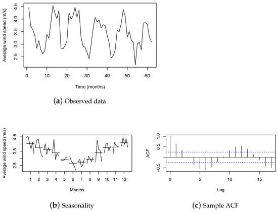
Figure 2. Time series of monthly WS in the city of Rio Grande in the period from December 2009 to January 2015.

To incorporate the seasonality pattern into the model, a covariate containing the deterministic seasonality component obtained from the decompose function of software R [26] was included in the fitted model. This function decomposed the time series into three components and estimated each one: trend, seasonality, and random. In addition, to determine the order of the models, we conducted a series of analyses using different combinations of $(p,q)$ orders and used the AIC and BIC to select the best one, followed by a residual analysis. The five best models according to the AIC and BIC are presented in Table 2. The most appropriate model was the CHARMA$(3,2)$ with a seasonal covariate. Table 3 presents the fitted model. We note that all the parameters were considered to be significant at the level of $10\%$.

Table 2. Information criteria for the five best CHARMA models fitted to the monthly WS time series.

Model	AIC	BIC
CHARMA$(3,2)$	$51.103$	$68.120$
CHARMA$(3,3)$	$52.846$	$71.990$
CHARMA$(2,3)$	$57.446$	$74.464$
CHARMA$(3,1)$	$62.170$	$77.060$
CHARMA$(1,0)$	$63.300$	$71.808$

Table 3. CHARMA$(3,2)$ model fitted to the WS time series in the city of Rio Grande from December 2009 to January 2015.

Parameter	Estimate	Std. Error	z Stat.	p-Value
${\beta }_0$	$2.475$	$0.469$	$5.279$	<$0.001$
${\varphi }_1$	$-1.121$	$0.119$	$9.445$	<$0.001$
${\varphi }_2$	$-0.277$	$0.166$	$1.668$	$0.095$
${\varphi }_3$	$0.393$	$0.113$	$3.464$	<$0.001$
${\theta }_1$	$1.571$	$0.076$	$20.670$	<$0.001$
${\theta }_2$	$0.879$	$0.089$	$9.872$	<$0.001$
${\beta }_1$	$0.274$	$0.035$	$7.757$	<$0.001$
$\lambda$	$1.623$	$0.054$	-	-
AIC = $51.103$ and BIC = $68.120$

Figure 3 presents the residual diagnostic plots of the fitted model. We can observe some indications that the model is capable of portraying the behavior of the data and is appropriate for out-of-sample forecasting. Figure 3a shows that the residuals are randomly distributed around zero without the presence of outliers. The quantile–quantile plot (QQ-Plot) in Figure 3b demonstrates a good fit, indicating that the residuals are approximately normally distributed. The residuals also do not show significant auto-correlation, as shown by the residual ACF in Figure 3c and the residual partial auto-correlation function (PACF) in Figure 3d. The Ljung-Box test confirms the goodness-of-fit with a p-value > $0.05$.

Figure 3. Diagnostic plots of the CHARMA$(3,2)$ model fitted to the WS time series.

For comparison purposes, we also considered the seasonal autoregressive moving average model (SARMA)$(p,q){(P,Q)}_S$ [1], where p and q represent the orders of the non-seasonal part of the model, P and Q are the orders of the seasonal part of the model, and $S=12$ is the period. After conducting a residual analysis and the Ljung-Box test, the SARMA$(2,3)\times {(2,0)}_{12}$ model was selected. In the SARMA fitted model, all the parameters were different from zero at a significance level of $5\%$. The model presented AIC and BIC values equal to $76.931$ and $96.076$, respectively.

In order to compare the fitted models, we evaluated the in-sample and out-of-sample predictions. For the out-of-sample evaluation, we reserved the last twelve observations solely for the purpose of comparing the forecasts. Figure 4 presents the time series of the mean WS together with the in-sample prediction and out-of-sample forecast of both competitor models. It can be observed that both models present a good fit in the time series.

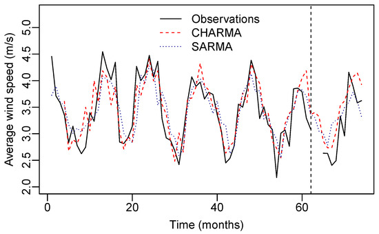
Figure 4. Observed and predicted WS values from the CHARMA$(3,2)$ and SARMA$(2,3)\times {(2,0)}_{12}$ models, which considered the fit period (in-sample) and the forecast period (out-of-sample) twelve steps ahead.

In Table 4, the observed and out-of-sample predicted values from the CHARMA and SARMA models are presented. It can be observed that the CHARMA model produces predictions that are close to the observed values of WS in five of the ten observations with recorded values. To further evaluate the predictive performance of the models, we calculated the MAPE% and the MSE between the observed and the fitted values. The results of these figure-of-merit measurements are presented in Table 5. It can be noted that the CHARMA model has the best performance in modeling the WS. When both measurements are considered, the selected model demonstrates the lowest values, indicating that it is the most suitable approach for modeling the WS dataset in the city of Rio Grande in the period from December 2009 to January 2016.

Table 4. Observed and forecast WS values for the CHARMA$(3,2)$ and SARMA$(2,3)\times {(2,0)}_{12}$ fitted models.

Period	Observations	CHARMA	SARMA
February (2015)	−	$3.401$	$3.305$
March (2015)	−	$3.322$	$3.046$
April (2015)	$2.633$	$2.861$	$3.003$
May (2015)	$2.630$	$2.736$	$2.786$
June (2015)	$2.404$	$2.734$	$3.187$
July (2015)	$2.493$	$3.037$	$3.254$
August (2015)	$3.332$	$3.532$	$3.283$
September (2015)	$2.959$	$3.616$	$3.493$
October (2015)	$4.158$	$3.857$	$3.589$
November (2015)	$3.895$	$4.068$	$3.782$
December (2015)	$3.581$	$4.148$	$3.612$
January (2016)	$3.623$	$3.927$	$3.323$

Table 5. In-sample and out-of-sample prediction accuracy measurements of the CHARMA($3,2)$ and SARMA$(2,3)\times {(2,0)}_{12}$ fitted models for the WS times series.

Models	MAPE (%)	MSE
In-sample
CHARMA$(3,2)$	$8.346$	$0.112$
SARMA$(2,3)\times {(2,0)}_{12}$	$8.710$	$0.133$
Out-of-sample
CHARMA$(3,2)$	$11.235$	$0.147$
SARMA$(2,3)\times {(2,0)}_{12}$	$12.837$	$0.207$

5.3. Application to Monthly Average Maximum Temperature Time Series in the City of Teresina

Climate is a determining factor for natural and human life. Variations in wind intensity, as well as temperature fluctuations, are important subjects in applied studies. According to [29], accurately predicting temperature is crucial for the prevention of unforeseen dangers caused by temperature variations, which can lead to human and financial losses. In this climatic context, statistical models are necessary to be able to analyze and predict variables while considering the serial dependence in the time series. The monthly average maximum temperature variable (or simply maximum temperature, abbreviated as MT) is an example of a parameter that enhances studies on climate change, wildfire prevention, and health problems. The CHARMA model is suitable for modeling this variable, given that the MT consists of a set of positive real values, and the model takes into account the temporal dependence structure of the data.

Brazil is known for having regions with high temperatures, such as the northeast region. To illustrate the applicability of the proposed model, we developed an empirical application of the proposed model using MT data taken from the capital of the Piauí estate, the city of Teresina, Brazil. The data were sourced from the INMET, available at https://bdmep.inmet.gov.br/ (accessed on 21 August 2023). The dataset comprised monthly observations from February 2010 to December 2015. This time period was selected to have the largest possible sample size, considering the missing values in the observed time series. The last nine observations were reserved only for the purpose of comparing the forecasting results, whereas the first $n=62$ observations were used for estimation. One of the last nine observations, corresponding to April 2015, was missing, and so the fitted models were used to input this missing value. Therefore, the time series used for estimation considered the period from February 2010 to March 2015, with $n=62$ observations, an average MT of $34.42$ °C, median of $33.86$ °C, the maximum temperature reached was $38.94$ °C, and the minimum was $31.72$ °C.

Figure 5 contains some graphs that indicate the behavior of the time series along the time period. Figure 5a shows the time series of MT, while Figure 5b evidences the seasonal pattern in the data. The sample ACF is shown in Figure 5c, which has been noted to have the presence of seasonality in the data. During the months of August and September, higher MT can be observed, whereas in the months from February to April, the temperatures are lower.

Figure 5. Time series of MT in the city of Teresina in the period from February 2010 to March 2015.

To be able to select the best model for the MT time series, we fitted the CHARMA$(p,q)$ models with different orders. In all the fitted models, we considered a covariate from the deterministic seasonality component obtained by the decompose R function. Table 6 presents the five models with the lowest AIC values among the competing models with different p and q orders. The model exhibiting the lowest AIC and BIC values was selected. Table 7 presents the adjustment of the CHARMA${(3,0)}^{*}$ model with a seasonal covariate. All parameters are considered to be significant at the significance level of 5%.

Table 6. Information criteria for the five best CHARMA models fitted to the MT time series.

Model	AIC	BIC
CHARMA${(3,0)}^{*}$	$121.111$	$131.746$
CHARMA$(1,3)$	$121.812$	$136.702$
CHARMA$(3,0)$	$121.878$	$134.641$
CHARMA${(3,1)}^{*}$	$122.255$	$135.018$
CHARMA$(3,1)$	$123.816$	$138.706$

${}^{*}$ represents the model with ${\varphi }_2=0$ because it did not reach the significance level of 5%.

Table 7. The CHARMA${(3,0)}^{*}$ model fitted to the MT time series for the city of Teresina from February 2010 to March 2015.

Parameter	Estimate	Std. Error	z Stat.	p-Value
${\beta }_0$	$0.890$	$0.376$	$2.369$	$0.018$
${\varphi }_1$	$0.451$	$0.087$	$5.160$	<$0.000$
${\varphi }_3$	$0.298$	$0.111$	$2.687$	$0.007$
${\beta }_1$	$0.026$	$0.001$	$21.648$	<$0.000$
$\lambda$	$1.143$	$0.022$	-	-
AIC = $121.111$ and BIC = $131.746$

Figure 6 shows some graphs for the diagnostic analysis of the fitted CHARMA${(3,0)}^{*}$. In Figure 6a, we can see that the residuals are randomly distributed between $(-3,3)$ without the presence of outliers. The QQ-Plot indicates that the Chen model is suitable for this application. Figure 6c,d and the Ljung-Box test (p-value $>0.05$) evidence that the residuals are not auto-correlated.

Figure 6. Diagnostic plots of the CHARMA${(3,0)}^{*}$ model fitted to the MT time series.

In order to compare the prediction performance of the proposed model with the most usual methodology in the time-series field [1], we used the auto.arima function from the package forecast of the software R. This function returns the best SARMA model, taking into account the AIC value of models with different order combinations, as well as autoregressive ($p\le 5$), moving averages ($q\le 5$), seasonal autoregressive ($P\le 2$), and seasonal moving averages ($Q\le 2$) terms. The model with the lowest AIC was ARMA$(2,1)$, with AIC$=173.690$ and BIC$=184.330$. Additionally, all model parameters were considered to be significant at the significance level of 5%. The Ljung-Box test for the fitted ARMA model residuals resulted in p-value$>0.005$; thus, the hypothesis assuming the independence of the residuals was not rejected.

For the comparison of the fitted CHARMA${(3,0)}^{*}$ and ARMA$(2,1)$ models, we evaluated the in-sample and out-of-sample predictions. The out-of-sample forecast is shown in Table 8. Note that the predicted values based on the proposed model are generally closer to the observed ones. Graphic representations of the in-sample and out-of-sample predictions can be seen in Figure 7.

Table 8. Observed and forecast MT values for the CHARMA${(3,0)}^{*}$ and ARMA$(2,1)$ fitted models.

Period	Observations	CHARMA	ARMA
April (2015)	-	$33.142$	$32.553$
May (2015)	$32.690$	$32.931$	$33.040$
June (2015)	$33.240$	$33.388$	$33.799$
July (2015)	$34.150$	$34.419$	$34.609$
August (2015)	$36.700$	$36.106$	$35.264$
September (2015)	$38.370$	$37.604$	$35.625$
October (2015)	$39.030$	$37.758$	$35.645$
November (2015)	$38.740$	$36.116$	$35.366$
December (2015)	$38.460$	$35.372$	$34.896$

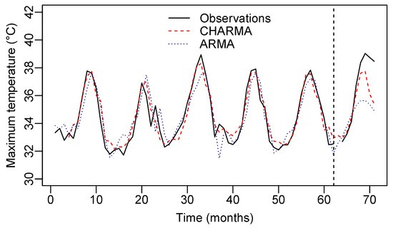
Figure 7. Observed and predicted MT values from the CHARMA${(3,0)}^{*}$ and ARMA$(2,1)$ models, which considered the fit period (in-sample) and the forecast period (out-of-sample) nine steps ahead.

Finally, the prediction accuracy measurements confirm the superiority of the CHARMA model, which can be seen in Table 9. In both in-sample and out-of-sample prediction measurements, the values of MAPE (%) and MSE are lower than those of the classical ARMA model.

Table 9. In-sample and out-of-sample prediction accuracy measurements of the CHARMA(${3,0)}^{*}$ and ARMA$(2,1)$ fitted models for the MT times series.

Models	MAPE (%)	MSE
In-sample
CHARMA${(3,0)}^{*}$	$1.349$	$0.340$
ARMA$(2,1)$	$2.002$	$0.790$
Out-of-sample
CHARMA${(3,0)}^{*}$	$2.956$	$2.391$
ARMA$(2,1)$	$5.227$	$5.723$

6. Conclusions

In this work, we proposed a dynamic model for modeling Chen-distributed and auto-correlated data. We introduced the median-based reparameterization of the Chen distribution, and we included a regression, autoregressive, and moving averages structure for the modeling of the conditional median. We discussed the model selection criteria and the use of quantile residuals to evaluate the model assumptions. The simulation results indicated that the conditional maximum likelihood estimators exhibit good properties in finite sample sizes. In addition to the theoretical proposition and the numerical evaluation of the introduced estimation theory, we verified the applicability of the proposed model on two real datasets of WS and MT. In both applications, the proposed CHARMA model demonstrated a good fit in terms of AIC, BIC, MAPE, and MSE, outperforming the classical SARMA and ARMA models in terms of prediction evaluation.

References

- Box, G.E.; Jenkins, G.M.; Reinsel, G.C.; Ljung, G.M. Time Series Analysis: Forecasting and Control; John Wiley & Sons: Hoboken, NJ, USA, 2015. [Google Scholar]
- Tiku, M.L.; Wong, W.K.; Vaughan, D.C.; Bian, G. Time series models in non-normal situations: Symmetric innovations. J. Time Ser. Anal. 2000, 21, 571–596. [Google Scholar] [CrossRef]
- Benjamin, M.A.; Rigby, R.A.; Stasinopoulos, D.M. Generalized autoregressive moving average models. J. Am. Stat. Assoc. 2003, 98, 214–223. [Google Scholar] [CrossRef]
- McCullagh, P.; Nelder, J. Generalized Linear Models, 2nd ed.; Chapman and Hall: London, UK, 1989. [Google Scholar]
- Rocha, A.V.; Cribari-Neto, F. Beta autoregressive moving average models. Test 2009, 18, 529–545. [Google Scholar] [CrossRef]
- Bayer, F.M.; Bayer, D.M.; Pumi, G. Kumaraswamy autoregressive moving average models for double bounded environmental data. J. Hydrol. 2017, 555, 385–396. [Google Scholar] [CrossRef]
- Melo, M.S.; Alencar, A.P. Conway-Maxwell-Poisson autoregressive moving average model for equidispersed, underdispersed, and overdispersed count data. J. Time Ser. Anal. 2020, 41, 830–857. [Google Scholar] [CrossRef]
- Sales, L.O.; Alencar, A.P.; Ho, L.L. The BerG generalized autoregressive moving average model for count time series. Comput. Ind. Eng. 2022, 168, 108104. [Google Scholar] [CrossRef]
- Bayer, F.M.; Pumi, G.; Pereira, T.L.; Souza, T.C. Inflated beta autoregressive moving average models. Comput. Appl. Math. 2023, 42, 183. [Google Scholar] [CrossRef]
- de Araújo, F.J.M.; Guerra, R.R.; Peña-Ramírez, F.A. The Burr XII autoregressive moving average model. Comput. Sci. Math. Forum 2023, 7, 46. [Google Scholar]
- Kedem, B.; Fokianos, K. Regression Models for Time Series Analysis; John Wiley & Sons: Hoboken, NJ, USA, 2005. [Google Scholar]
- Chen, Z. A new two-parameter lifetime distribution with bathtub shape or increasing failure rate function. Stat. Probab. Lett. 2000, 49, 155–161. [Google Scholar] [CrossRef]
- Xie, M.; Tang, Y.; Goh, T. A modified Weibull extension with bathtub-shaped failure rate function. Reliab. Eng. Syst. Saf. 2002, 76, 279–285. [Google Scholar] [CrossRef]
- Dey, S.; Kumar, D.; Ramos, P.L.; Louzada, F. Exponentiated Chen distribution: Properties and estimation. Commun. Stat. Simul. Comput. 2017, 46, 8118–8139. [Google Scholar] [CrossRef]
- Alotaibi, R.; Rezk, H.; Park, C.; Elshahhat, A. The discrete exponentiated-Chen model and its applications. Symmetry 2023, 15, 1278. [Google Scholar] [CrossRef]
- Press, W.H.; Teukolsky, S.A.; Vetterling, W.T.; Flannery, B.P. Numerical Recipes in C. 2; Cambrige University: Cambridge, UK, 1992. [Google Scholar]
- Andersen, E.B. Asymptotic properties of conditional maximum-likelihood estimators. J. R. Stat. Soc. Ser. B Methodol. 1970, 32, 283–301. [Google Scholar] [CrossRef]
- Fokianos, K.; Kedem, B. Partial likelihood inference for time series following generalized linear models. J. Time Ser. Anal. 2004, 25, 173–197. [Google Scholar] [CrossRef]
- Akaike, H. A new look at the statistical model identification. IEEE Trans. Autom. Control 1974, 19, 716–723. [Google Scholar] [CrossRef]
- Dunn, P.K.; Smyth, G.K. Randomized quantile residuals. J. Comput. Graph. Stat. 1996, 5, 236–244. [Google Scholar]
- Scott, M.; Chandler, R. Statistical Methods for Trend Detection and Analysis in the Environmental Sciences; John Wiley & Sons: Hoboken, NJ, USA, 2011. [Google Scholar]
- Ljung, G.M.; Box, G.E. On a measure of lack of fit in time series models. Biometrika 1978, 65, 297–303. [Google Scholar] [CrossRef]
- Prass, T.S.; Bravo, J.M.; Clarke, R.T.; Collischonn, W.; Lopes, S.R. Comparison of forecasts of mean monthly water level in the Paraguay River, Brazil, from two fractionally differenced models. Water Resour. Res. 2012, 48, 5. [Google Scholar] [CrossRef]
- Abdel-Aal, R. Univariate modeling and forecasting of monthly energy demand time series using abductive and neural networks. Comput. Ind. Eng. 2008, 54, 903–917. [Google Scholar] [CrossRef]
- Suganthi, L.; Samuel, A.A. Energy models for demand forecasting—A review. Renew. Sustain. Energy Rev. 2012, 16, 1223–1240. [Google Scholar] [CrossRef]
- R Core Team. R: A Language and Environment for Statistical Computing; R Foundation for Statistical Computing: Vienna, Austria, 2022. [Google Scholar]
- Zhang, L.; Zhou, D.Q.; Zhou, P.; Chen, Q.T. Modelling policy decision of sustainable energy strategies for Nanjing City: A fuzzy integral approach. Renew. Energy 2014, 62, 197–203. [Google Scholar] [CrossRef]
- Wang, C.; Prinn, R.G. Potential climatic impacts and reliability of very large-scale wind farms. Atmos. Chem. Phys. 2010, 10, 2053–2061. [Google Scholar] [CrossRef]
- Paul, R.K.; Anjoy, P. Modeling fractionally integrated maximum temperature series in India in presence of structural break. Theor. Appl. Climatol. 2018, 134, 241–249. [Google Scholar] [CrossRef]
Disclaimer/Publisher’s Note: The statements, opinions and data contained in all publications are solely those of the individual author(s) and contributor(s) and not of MDPI and/or the editor(s). MDPI and/or the editor(s) disclaim responsibility for any injury to people or property resulting from any ideas, methods, instructions or products referred to in the content. |
© 2023 by the authors. Licensee MDPI, Basel, Switzerland. This article is an open access article distributed under the terms and conditions of the Creative Commons Attribution (CC BY) license (https://creativecommons.org/licenses/by/4.0/).