Edge Resolvability in Generalized Petersen Graphs

Abstract

The generalized Petersen graphs are a type of cubic graph formed by connecting the vertices of a regular polygon to the corresponding vertices of a star polygon. This graph has many interesting graph properties. As a result, it has been widely researched. In this work, the edge metric dimensions of the generalized Petersen graphs GP(2l + 1, l) and GP(2l, l) are explored, and it is shown that the edge metric dimension of GP(2l + 1, l) is equal to its metric dimension. Furthermore, it is proved that the upper bound of the edge metric dimension is the same as the value of the metric dimension for the graph GP(2l, l).

1. Introduction

The study of resolving sets and locating sets in graphs, introduced by Slater and later independently researched by Harary and Melter, has opened up fascinating possibilities in network analysis. A metric generator R, defined as a vertex subset of a given graph, holds the unique capability of precisely determining the distance between vertices. Notably, Slater demonstrated how this concept could be leveraged to pinpoint the location of an intruder within a network. What happens, then, if we want to locate an intrusion without relying simply on the nodes or vertices? This intriguing question prompted further investigation. Kelenc et al. [1] took the initiative to develop the concept of edge resolvability in graphs, adding an additional condition to tackle this problem. Their work not only extended the idea of vertex resolving sets but also delved into the realm of edge resolving sets, unveiling a multitude of metric features.

Let $V\left(G\right)$ and $E\left(G\right)$ denote the node (or vertex) set and edge set of a simple, undirected and connected graph $G$. With the help of a distance parameter, the nodes and edges of graph $G$ are identified. In graph $G$, the distance between a graph node $\alpha$ and an edge $\beta ={\alpha }_1{\alpha }_2$ is given by $d_G(\beta ,\alpha )=\mathrm{m}\mathrm{i}\mathrm{n}\left\{d_G\right({\alpha }_1,\alpha ),d_G({\alpha }_2,\alpha \left)\right\}$. A graph’s vertex $\alpha$ is said to resolve any two edges ${\beta }_1$ and ${\beta }_2$ of a graph $G$ whenever $d_G(\alpha ,{\beta }_1)\ne d_G(\alpha ,{\beta }_2)$. A code for an edge $\mathsf{\beta }$ with respect to the set $W=\{a_1,\dots ,a_n\}$ is defined as ${\mathrm{c}}_{\mathrm{W}}\left(\beta \right)=(\mathrm{d}\left({\mathrm{a}}_1, \beta \right),\dots , d\left(a_n,\beta \right))$. W is said to be an edge resolving set if all the edges have distinct codes.

Definition 1. 

A subset of a vertex set is said to be an edge resolving set if every vertex in the subset can resolve all the edges of G. An edge resolving set with minimum cardinality is called an edge basis. The number of elements in the edge basis is called the edge metric dimension of G. The symbol ${\beta }_e\left(G\right)$ then denotes the edge metric dimension of graph G  [1].

The edge metric dimensions of the generalized Petersen graphs $\mathrm{G}\mathrm{P}$($2\mathrm{l}+1,\mathrm{l}$) and $GP(2l,l)$ are determined in this work, and it is demonstrated that ${\beta }_e\left(G\mathrm{P}\left(2\mathrm{l}+1,\mathrm{l}\right)\right)$ is equal to the metric dimension of $\mathrm{G}\mathrm{P}$($2\mathrm{l}+1,\mathrm{l}$). Furthermore, it is demonstrated that the upper bound value of the edge metric dimension is the same as the value of the metric dimension for the graph $\mathrm{G}\mathrm{P}(2\mathrm{l},\mathrm{l})$. In this work, the subscripts are taken as modulo $l.$

2. Applications

Applications for resolvability in graphs include pattern recognition, image processing, and robot network navigation [2]. Additionally, it has numerous uses in drug and pharmaceutical chemistry [3,4,5]. Mastermind game and coin weighing problems have many interesting links with the metric generators of graphs that were presented in [6].

For the application to robot navigation, the robot is assumed to be moving from vertex to vertex in a graph, with some vertices designated as landmarks. The robot can calculate its distance from each landmark and use that information to determine its position in the graph. The goal is to use as few landmarks as possible, and the metric dimension is the number of landmarks used. In [1], a parameter closely related to metric dimension was recently defined. Consider that the robot is now moving from edge to edge rather than vertex to vertex. The robot can still determine its distance from the landmarks, where the distance from an edge to a landmark is the shortest distance from or to the landmark. Again, the goal is to use as few landmarks as possible, and that number is the edge metric dimension.

The metric dimension for a number of graphs is either equal to, less than or greater than the edge metric dimension [7].

The following example emphasizes the importance of edge metric dimensions in real life.

Example 1. 

The concept of a metric generator was used by Slater [8] to determine the location of an intruder in a network in a unique way. There are several distinct types of metric generators in graphs today, and each one is being investigated both theoretically and practically, depending on its use or popularity. However, quite a few more viewpoints still exist that are not fully taken into consideration when defining a graph using these metric generators. Consider a network whose vertices may be known to be uniquely identified by a metric generator. Then, correct vertex surveillance is operational. However, if a hacker gains access to the network not through its vertices but rather through links between them (edges), they will not be able to be located, and in this case, the surveillance fails to live up to its promise and more network infrastructure is needed. In light of these facts, we develop and examine a novel type of metric generator in this work in an effort to advance our understanding of these distance-related metrics in graphs.

Motivated by this, Kelenc et al. [1] defined the concept of edge resolvability in graphs and studied its different metric properties.

Further, the concept of lower and upper bounds is an important tool in mathematical analysis, optimization and decision-making, as it allows us to determine the range of possible values for a quantity and identify the optimal value within that range. For example, in structural engineering, lower and upper bound theorems are used to predict design loads. The lower bound is used to predict the minimum load at which there is an onset of plastic deformation or plastic hinge formation at any point in the structure. Understandably, the first plastic hinges will form at points with the highest ratio of applied moment to flexural rigidity.

Plastic hinges cause excessive rotation and deformation, much more than that caused while the structure is in elastic range. But this deformation does not destabilize the structure, because the structures designed using plastic theorems are mostly indeterminate or over-supported. A hinge formation, in essence, adds a degree of freedom to the otherwise over-constrained or over-supported structure until a time when a sufficient number of plastic hinges are formed to finally destabilize the structure and cause its collapse. This is called a mechanism wherein the collapse follows a certain constraint relationship dictated by the geometry of the structure and the location of the plastic hinges. The upper bound is used to predict the load that shall cause such a mechanism to form.

It follows that between these two values of load given by the lower and upper bound theorem lies the collapse load, and the design load is based on this collapse load with some factor of safety. Below the lower bound, the structure would be perfectly safe with no onset of plasticity and large reserve strength; between the lower and upper bounds, some plastic hinges shall form and deformations shall increase, causing serviceability concerns, but the structure would otherwise still perform its intended function; above the upper bound, plastic hinges will cause mechanisms to form and cause the structure to collapse.

Lemma 1. 

$\beta \left(P_l\right)={\beta }_e\left(P_l\right)=1,$ for any integer $l$ $\ge 2$. Moreover, ${\beta }_e\left(G\right)=1$ if, and only if, $G$ = $P_l$ [1].

The following remark can be deduced from the above Lemma.

Remark 1. 

If G is a non-trivial and connected graph $(G\ne P_n)$ with $n$ vertices, then ${\beta }_e\left(G\right)\ge 2$.

There are several metric properties in the generalized Petersen graph. The resolvability of $\mathrm{G}\mathrm{P}(\mathrm{l},\mathrm{p})$ and $\mathrm{G}\mathrm{P}(\mathrm{l},\mathrm{p})$ for $p=3$ and $4$ was studied in [8] and [9], respectively. The edge resolvability of $\mathrm{G}\mathrm{P}(\mathrm{l},\mathrm{p})$ and $\mathrm{G}\mathrm{P}(\mathrm{l},\mathrm{p})$ for $p=1$ and $2$ was computed separately in [10] and [11]. The graphs $\mathrm{G}\mathrm{P}(2\mathrm{l}+1,\mathrm{l})$ and $\mathrm{G}\mathrm{P}(2\mathrm{l},\mathrm{l})$ have metric dimension $3$ and $4$, as detailed in [12] and [13], respectively. Moreover, the edge metric dimensions of a $k$-multi wheel graph, some subdivisions of the wheel graph, convex polytopes, Cayley graphs and its barycentric subdivisions and the metric dimension of Cayley digraphs of split metacyclic groups were studied in [14,15,16,17]. Further results on metric and edge metric dimensions can be found in [18,19,20,21,22,23,24].

3. Results

In this paper, we investigate the edge metric dimension of some families of graphs, namely, $\mathrm{G}\mathrm{P}(2\mathrm{l}+1,\mathrm{l})$ and $\mathrm{G}\mathrm{P}(2\mathrm{l},\mathrm{l})$. We start this section with a new result regarding the edge metric dimension of the graph $\mathrm{G}\mathrm{P}(2\mathrm{l}+1,\mathrm{l})$ in the following theorems. In the following section, the results regarding the edge metric dimension of $\mathrm{G}\mathrm{P}(2\mathrm{l},\mathrm{l})$ are discussed.

Generalized Petersen Graph

The well-known family of 3-regular graphs are generalized Petersen graphs, which have drawn much attention in graph theory because of their numerous practical uses. With $2n$ vertices and $3n$ edges, the generalized Petersen graph $\mathrm{G}\mathrm{P}(\mathrm{n},\mathrm{q})$: 1 $\le q \le ⌊\frac{n}{2}⌋$ is created as follows:

Draw an n-length cycle and denote the vertices of the cycle by $r_1,\dots ,r_n$. Again, draw a pendent vertex $s_i$ adjacent to each vertex $r_i$. Finally, join each vertex $s_i$ to vertex $s_j$ by an edge such that $|i-j|=q$. The graph obtained by the above construction is the generalized Petersen graph $\mathrm{G}\mathrm{P}(\mathrm{n},\mathrm{q})$. 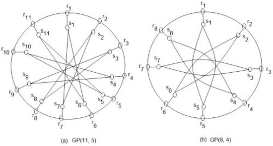The graphs of $\mathrm{G}\mathrm{P}\left(\mathrm{11,5}\right)$ and $\mathrm{G}\mathrm{P}\left(\mathrm{8,4}\right)$ are shown in Figure 1.

The following bound was stated in [14] for all t-regular graphs.

Lemma 2. 

If $G$ is a $t$-regular graph, then ${\beta }_e\left(G\right)\ge 1+\lceil lo{g}_{2}t\rceil$ [8].

As we know that $GP\left(n,q\right)$ is a $3$-regular graph, and $⌈lo{g}_{2}3⌉=2,$ the next lemma also holds.

Lemma 3. 

For any generalized Petersen graph $GP(n,q)$, ${\beta }_e\left(GP\left(n,q\right)\right)\ge 3$.

Lemma 4. 

For all $l\ge 12$ where $l$ is even, ${\beta }_e\left(GP\right(2l+1,l\left)\right)\le 3$.

Proof. 

Let $W=\left\{r_1,r_{⌈\frac{2l+1}{2}⌉},s_{⌈\frac{3l}{2}⌉}\right\}$. Let $k_1=⌊\frac{l}{3}⌋$, $t_1=\frac{l}{2}$ and $l_1=\lceil \frac{q}{6}\rceil -1$. In order to prove that W is an edge resolving set, it is necessary to show that all the edges of the graph $\mathrm{G}\mathrm{P}(2\mathrm{l}+1,\mathrm{l})$ can be resolved from the vertices of W. To this end, all of the codes for the edges of $\mathrm{G}\mathrm{P}(2\mathrm{l}+1,\mathrm{l})$ with regard to W are listed in

Table 1. The codes of outer edges $r_{d_2}{r}_{d_2+1}$.

Edges	Codes
$r_{p_2}{r}_{d_2+1}, d_2\in \{\mathrm{1,2},\dots ,t_1-2\}$	$(d_2-1,d_2+2,t_1-d_2)$
$r_{d_2}{r}_{d_2+1}, d_2=t_1-1$	$(d_2-1,d_2+2,2)$
$r_{d_2}{r}_{d_2+1}, d_2\in \{t_1,1+t_1,2+t_1\}$	$(d_2-1,\hspace{1em} l-d_2,3+d_2-\lceil \frac{2\mathrm{l}+1}{4}\rceil )$
$r_{d_2}{r}_{d_2+1}, d_2\in \{t_1+3,t_1+4,\dots ,l-1\}$	$(3+l-d_2,l-d_2,d_2+3-\lceil \frac{2\mathrm{l}+1}{4}\rceil )$
$r_{d_2}{r}_{d_2+1}, d_2\in \{l,\mathrm{l}+1\}$	$(3,0, \lceil \frac{2l+1}{2}\rceil +l_1+k_1-d_2)$
$r_{d_2}{r}_{d_2+1}, d_2\in \{l+2,l+3,\dots ,3t_1-1\}$	$(d_2+1-l,{ d}_2-l-1,2l+1-d_2-k_1-l_1-2)$
$r_{d_2}{r}_{d_2+1}, d_2=3t_1$	$({1+d}_2-l,d_2-l-1,1)$
$r_{d_2}{r}_{d_2+1}, d_2=1+3t_1$	$(d_2-(1+l),d_2-(1+l),2)$
$r_{d_2}{r}_{d_2+1}, d_2\in \{3t_1+2,\dots ,2l\}$	$(1+2l-d_2,3+2l-d_2,d_2-(l+k_1+l_1\left)\right)$
$r_{d_2}{r}_{d_2+1}, d_2=1+2l$	$(0,3,t_1)$

,

Table 2. The codes of outer edges $r_{d_2}{r}_{d_2+1}$.

Edges	Codes
$r_{d_2}{s}_{d_2}, d_2\in \{\mathrm{1,2},\dots ,t_1-2\}$	$(d_2-\mathrm{1,2}+d_2,\lceil \frac{2l+1}{4}\rceil -d_2)$
$r_{d_2}{s}_{d_2}, d_2\in \{t_1-1,t_1\}$	$(d_2-\mathrm{1,1}+d_2,1)$
$r_{d_2}{s}_{d_2}, d_2\in \{1+t_1,2+t_1\}$	$(d_2-1,1+l-d_2,1+d_2-(k_1+l_1\left)\right)$
$r_{d_2}{s}_{d_2}, d_2\in \{3+t_1,4+t_1,\dots ,l-1\}$	$(3+l-d_2,1+l-d_2,2+d_2-t_1)$
$r_{d_2}{s}_{d_2}, d_2=l+t_1$	$(d_2-l,d_2-l-1,0)$
$r_{d_2}{s}_{d_2}, d_2\in \{1+l+t_1,2+\mathrm{l}+t_1\}$	$(2+2l-d_2,d_2-l-\mathrm{1,1}+d_2-l-t_1)$
$r_{d_2}{s}_{d_2}, d_2\in \{q+t_1+3,\dots ,2l\}$	$(2+2l-d_2,3+2l-d_2,d_2-(l+k_1+l_1\left)\right)$
$r_{d_2}{s}_{d_2}, d_2=1+2l$	$(2+2l-d_2,3+2l-d_2,1+t_1)$

,

Table 3. The codes of inner edges $s_{d_2}{s}_{d_2+l}$.

Edges	Codes
$s_{2l+3-d_2}{s}_{l+2-d_2}, d_2=2$	$(d_2,d_2,2+t_1)$
$s_{2l+3-d_2}{s}_{l+2-d_2,} d_2\in \{\mathrm{3,4},\dots ,t_1\}$	$(d_2,d_2,l-l_1-d_2-k_1+4)$
$s_{2l+3-d_2}{s}_{l+2-d_{2,}} d_2=1+t_1$	$(d_2,d_2,3)$
$s_{2l+3-d_2}{s}_{l+2-d_2}, d_2=t_1$ +2	$(2+l-d_2,l+3-d_2,1)$
$s_{2l+3-d_2}{s}_{l+2-d_2}, d_2=3+t_1$	$(l+2-d_2,3+l-d_2,0)$
$s_{2l+3-d_2}{s}_{l+2-d_2}, d_2=4+t_1$	$(l+2-d_2,3+l-d_2,2)$
$s_{2l+3-d_2}{s}_{l+2-d_2}, d_2=5+t_1$	$(l+2-d_2,3+l-d_2,4)$
$s_{2l+3-d_2}{s}_{l+2-d_2}, d_2\in \{6+t_1,7+t_1,\dots ,1+l\}$	$(l+2-d_2,3+l-d_2,l_1+d_2+k_1-l)$

and

Table 4. The codes of inner edges $s_{d_2}{s}_{d_2+l}$.

Edges	Codes
$s_{l+2-d_2}{s}_{2\mathrm{l}+2-d_2},$$d_2\in \{\mathrm{2,3},\dots ,t_1\}$	$(1+d_2,d_2,4+t_1-d_2)$
$s_{l+2-d_2}{s}_{2\mathrm{l}+2-d_2,}$$d_2=1+t_1$	$(d_2,d_2,2)$
$s_{l+2-d_2}{s}_{2\mathrm{l}+2-d_2},$$d_2\in \{2+t_1,3+t_1\}$	$(2+l-d_2,l+2-d_2,d_2-t_1-2)$
$s_{l+2-d_2}{s}_{2\mathrm{l}+2-d_2},$$d_2=4+t_1$	$(2+l-d_2,l+2-d_2,3)$
$s_{l+2-d_2}{s}_{2\mathrm{l}+2-d_2},$$d_2\in \{5+t_1,\dots ,l\}$	$(2+l-d_2,l+2-d_2,l_1+1+k_1+d_2-l)$

.

The codes of the spokes are given as follows.

When $l\equiv 0(\mathrm{m}\mathrm{o}\mathrm{d} 3)$ and is even,

$${\mathrm{c}}_{\mathrm{W}}\left({\mathrm{r}}_{{\mathrm{p}}_2}{\mathrm{s}}_{{\mathrm{p}}_2}\right)=(3+l-{\mathrm{p}}_2,1+l-{\mathrm{p}}_2,l+2{\mathrm{k}}_1-l_1-{\mathrm{p}}_2),(l\le {\mathrm{p}}_2\le l+1)$$

and

$${\mathrm{c}}_{\mathrm{W}}\left({\mathrm{r}}_{{\mathrm{p}}_2}{\mathrm{s}}_{{\mathrm{p}}_2}\right)=({\mathrm{p}}_2-l,{\mathrm{p}}_2-l-1,l+2{\mathrm{k}}_1-1-{\mathrm{p}}_2),\mathrm{w}\mathrm{h}\mathrm{e}\mathrm{r}\mathrm{e} (l+2\le {\mathrm{p}}_2\le l+{\mathrm{t}}_1-1).$$

When $l\equiv 1(\mathrm{m}\mathrm{o}\mathrm{d} 3)$ and is even,

$${\mathrm{c}}_{\mathrm{W}}\left({\mathrm{r}}_{{\mathrm{p}}_2}{\mathrm{s}}_{{\mathrm{p}}_2}\right)=(3+l-{\mathrm{p}}_2,1+l-{\mathrm{p}}_2,l+2{\mathrm{k}}_1+1-{\mathrm{l}}_1-{\mathrm{p}}_2),(l\le {\mathrm{p}}_2\le \mathrm{l}+1)$$

and

$${\mathrm{c}}_{\mathrm{W}}\left({\mathrm{r}}_{{\mathrm{p}}_2}{\mathrm{s}}_{{\mathrm{p}}_2}\right)=({\mathrm{p}}_2-l,{\mathrm{p}}_2-l-1,l+2{\mathrm{k}}_1+1-1_1-{\mathrm{p}}_2),(l+2\le {\mathrm{p}}_2\le l+{\mathrm{t}}_1-1).$$

When $l\equiv 2(\mathrm{m}\mathrm{o}\mathrm{d} 3)$ and is even,

$${\mathrm{c}}_{\mathrm{W}}\left({\mathrm{r}}_{{\mathrm{p}}_2}{\mathrm{s}}_{{\mathrm{p}}_2}\right)=(3+l-{\mathrm{p}}_2,1+l-{\mathrm{p}}_2,l+2{\mathrm{k}}_1+2-{\mathrm{l}}_1-{\mathrm{p})}_2,(l\le {\mathrm{p}}_2\le l+1).$$

and

$${\mathrm{c}}_{\mathrm{W}}\left({\mathrm{r}}_{{\mathrm{p}}_2}{\mathrm{s}}_{{\mathrm{p}}_2}\right)=\left({\mathrm{p}}_2-l,{\mathrm{p}}_2-l-1,l+2{\mathrm{k}}_1+2-1-{\mathrm{p}}_2\right),(l+2\le {\mathrm{p}}_2\le l+{\mathrm{t}}_1-1).$$

Moreover, when $l\equiv 0,2\left(\mathrm{m}\mathrm{o}\mathrm{d} 3\right),$

$${\mathrm{c}}_{\mathrm{W}}\left({\mathrm{s}}_1{s}_{l+1}\right)=(1,1,{\mathrm{t}}_1+1), {\mathrm{c}}_{\mathrm{W}}\left(s_{l+1}{s}_{2l+1}\right)=\left(2,1,{\mathrm{t}}_1+1\right).$$

and if $l\equiv 1(\mathrm{m}\mathrm{o}\mathrm{d} 3)$, then

$${\mathrm{c}}_{\mathrm{W}}\left({\mathrm{s}}_1{s}_{l+1}\right)=(1,1,{\mathrm{t}}_1+1), {\mathrm{c}}_{\mathrm{W}}\left(s_{l+1}{s}_{2l+1}\right)=(2,1,{\mathrm{t}}_1).$$

All of the edges then have unique codes with respect to the set W. Therefore, W is an edge resolving set. Further, W has cardinality three; therefore,

$${\beta }_e \left(GP\right(2l+1, l\left)\right)\le 3$$

(1)

□

Lemma 5. 

When $l$ is odd and $l$ $\ge 11$, ${\beta }_e\left(GP\right(2l+1,l\left)\right)\le 3$.

Proof. 

Let $\mathrm{W}=\left\{r_1,r_{⌈\frac{2l+1}{2}⌉},s_{⌈\frac{3l}{2}⌉}\right\}$,${\mathrm{k}}_1=\lfloor l/3\rfloor$ and ${\mathrm{t}}_1=\lceil \frac{l}{2}\rceil$. Further, when $l\equiv \mathrm{0,1} \left(mod3\right)$, ${\mathrm{l}}_1=\lceil l/6\rceil -1$, and when $l\equiv 2(mod 3)$, ${\mathrm{l}}_1=\lceil \frac{l}{6}\rceil$. In order to prove that W is an edge resolving set, it is necessary to show that all the edges of the graph $\mathrm{G}\mathrm{P}(2l+1, l)$ can be resolved from the vertices of W. To this end, all of the codes for the edges of $\mathrm{G}\mathrm{P}(2\mathrm{l},\mathrm{l})$ with regard to W are listed in

Table 5. The codes of outer edges $r_{d_2}{r}_{d_2+1}$.

Edges	Codes
$r_{d_2}{r}_{d_2+1}, d_2\in \{\mathrm{1,2},\dots ,t_1-2\}$	$(d_2-\mathrm{1,2}+d_2,t_1-d_2)$
$r_{d_2}{r}_{d_2+1}, d_2=t_1-1$	$(d_2-\mathrm{1,1}+d_2,2)$
$r_{d_2}{r}_{d_2+1}, d_2\in \{t_1,t_1+1\}$	$(d_2-1,l-d_2,2+d_2-\lceil (2l+1)/4\rceil )$
$r_{d_2}{r}_{d_2+1}, d_2\in \{t_1+2,\dots ,l-1\}$	$\left(3+l-d_2, l-d_2,2+d_2-⌈\frac{2l+1}{4}⌉\right)$
$r_{d_2}{r}_{d_2+1}, d_2\in \{l,l+1\}$	$(3,0, ⌈\frac{2l+1}{2}⌉+k_1+l_1-d_2)$
$r_{d_2}{r}_{d_2+1}, d_2\in \{2+l,\dots ,l+k_1+l_1\}$	$(1+d_2-l,d_2-l-\mathrm{1,1}+l+k_1+l_1-d_2)$
$r_{d_2}{r}_{d_2+1}, d_2\in \{l+k_1+l_1+1,l+k_1+l_1+2\}$	$(1+2l-d_2,d_2-l-1,d_2-l-k_1-l_1)$
$r_{d_2}{r}_{d_2+1}, d_2\in \{l+k_1+l_1+3,\dots ,2l\}$	$(1+2l-d_2,3+2l-d_2,d_2-l-k_1-l_1)$
$r_{d_2}{r}_{d_2+1}, d_2=1+2l$	$(0,3,t_1)$

,

Table 6. The codes of outer edges $r_{d_2}{r}_{d_2}$.

Edges	Codes
$r_{d_2}{s}_{d_2}, d_2\in \{1,\dots ,t_1-2\}$	$(d_2-\mathrm{1,1}+d_2,1+\lceil \frac{2l+1}{4}\rceil -d_2)$
$r_{d_2}{s}_{d_2}, d_2\in \{t-1,t_1\}$	$(d_2-1,t_1,1)$
$r_{d_2}{s}_{d_2}, d_2\in \{t_1+1,t_1+2\}$	$(t_1,l+1-d_2,2+d_2-t_1)$
$r_{d_2}{s}_{d_2}, d_2\in \{t_1+3,\dots ,l\}$	$(3+l-d_2,l+1-d_2,2+d_2-t_1)$
$r_{d_2}{s}_{d_2}, d_2=1+l$	$(2,0, t_1)$
$r_{d_2}{s}_{d_2}, d_2=l+t_1$	$(t_1,t_1-1,0)$
$r_{d_2}{s}_{d_2}, d_2=1+l+t_1$	$(2+2l-d_2,2l+2-d_2,2)$
$r_{d_2}{s}_{d_2}, d_2\in \{2+l+t_1,\dots ,2l+1\}$	$(2+2l-d_2,3+2l-d_2,1+d_2-l-t_1)$

,

Table 7. The codes of inner edges $s_{d_2}{s}_{d_2+l}$.

Edges	Codes
$s_{2l+3-d_2}{s}_{2+l-d_2}, d_2\in \{2,\dots ,t_1-1\}$	$(d_2,d_2,4+q-k-l_1-d_2)$
$s_{2l+3-d_2}{s}_{2+l-d_2}, d_2=t_1$	$(d_2,d_2,1+l_1)$
$s_{2l+3-d_2}{s}_{2+l-d_2}, d_2=t_1$+1	$(l+2-d_2,3+l-d_2,1)$
$s_{2l+3-d_2}{s}_{2+l-d_2}, d_2=t_1$+2	$(l+2-d_2,3+l-d_2,0)$
$s_{2l+3-d_2}{s}_{2+l-d_2}, d_2=t_1$+3	$(l+2-d_2,3+l-d_2,2)$
$s_{2l+3-d_2}{s}_{2+l-d_2}, d_2\in \{4+t_1,\dots ,l+l_1\}$	$(2+l-d_2,3+l-d_2,l_1+k+d_2-l)$

and

Table 8. The codes of inner edges $s_{d_2}{s}_{d_2+l}$.

Edges	Codes
$s_{2+l-d_2}{s}_{2+2\mathrm{l}-d_2}, d_2\in \{2,\dots ,t_1-1\}$	$(1+d_2,d_2,3+t_1-d_2)$
$s_{2+l-d_2}{s}_{2+2l-d_2}, d_2=t_1$	$(1+d_2,d_2,2)$
$s_{2+l-d_2}{s}_{2+2l-d_2}, d_2=1+t_1$	$(d_2-1,d_2-\mathrm{1,0})$
$s_{2+l-d_2}{s}_{2+2l-d_2}, d_2=2+t_1$	$(d_2-3,d_2-\mathrm{3,1})$
$s_{2+l-d_2}{s}_{2+2\mathrm{l}-d_2}, d_2=3+t_1$	$(2+l-d_2, 2+l-d_2,3)$
$s_{2+\mathrm{l}-d_2}{s}_{2\mathrm{l}+2-d_2}, d_2\in \{4+t_1,\dots ,l\}$	$(\mathrm{l}+2-d_2,l+2-d_2,l_1+1+k+d_2-l)$

.

Moreover, when $l\equiv 0(\mathrm{m}\mathrm{o}\mathrm{d} 3)$, then

$${\mathrm{c}}_{\mathrm{W}}\left({\mathrm{r}}_{{\mathrm{p}}_2}{\mathrm{s}}_{{\mathrm{p}}_2}\right)=({\mathrm{p}}_2-l,{\mathrm{p}}_2-l-1,l+{\mathrm{t}}_1+l_1-{\mathrm{p}}_2,l+2\le {\mathrm{p}}_2\le l+{\mathrm{t}}_1-1).$$

When $l\equiv 1,2\left(\mathrm{m}\mathrm{o}\mathrm{d} 3\right)$ and is odd,

$${\mathrm{c}}_{\mathrm{W}}\left({\mathrm{r}}_{{\mathrm{p}}_2}{\mathrm{s}}_{{\mathrm{p}}_2}\right)=({\mathrm{p}}_2-l,{\mathrm{p}}_2-l-1,l+{\mathrm{t}}_1+l_1-{\mathrm{p}}_2-2,l+2\le {\mathrm{p}}_2\le l+{\mathrm{t}}_1-1).$$

Further, $c_W\left(s_1{s}_{l+1}\right)=(1,1,t_1+1)$ and $c_W\left(s_{l+1}{s}_{2l+1}\right)=(2,1,t_1+1)$. All of the edges have distinctive codes, as can be seen. Therefore, W is an edge resolving set for $\mathrm{G}\mathrm{P}(2\mathrm{l}+1,\mathrm{l})$. Hence,

$${\beta }_e \left(GP\right(2l+1, l\left)\right)\le 3$$

(2)

□

Theorem 1. 

For $l\ge 11$, ${\beta }_e\left(GP\left(2l+1, l\right)\right)=3$.

Proof. 

The lower bound follows from Lemma 2, and the upper bound follows from Lemmas 4 and 5. □

The next result gives the upper bound for $\mathrm{G}\mathrm{P}(2\mathrm{l},\mathrm{l})$.

Lemma 6. 

For $l\equiv \mathrm{0,2}(mod 4)$ and $l\ge 8$, ${\beta }_e\left(GP\right(2l, l\left)\right)\le 3$.

Proof. 

Let $W=\left\{r_1,s_{\frac{l}{2}},s_l\right\}$ and $k_2=\frac{l}{2}$. In order to prove that W is an edge resolving set, it is necessary to show that all the edges of the graph $\mathrm{G}\mathrm{P}(2l+1, l)$ can be resolved from the vertices of W. To this end, all of the codes for the edges of $\mathrm{G}\mathrm{P}(2\mathrm{l},\mathrm{l})$ with regard to W are listed in

Table 9. The codes of outer edges $r_{d_2}{r}_{d_2+1}$.

Edges	Codes
$r_{d_2}{r}_{d_2+1}, d_2\in \{1,\dots ,k_2-1\}$	$(d_2-1,k_2-d_2,2+d_2)$
$r_{d_2}{r}_{d_2+1}, d_2\in \{k_2,k_2+2\}$	$(d_2-\mathrm{1,1}+d_2-k_2,\mathrm{l}-d_2)$
$r_{d_2}{r}_{d_2+1}, d_2\in \{k_2+3,\dots ,l-1\}$	$(3-d_2+l,d_2+1-k_2,\mathrm{l}-d_2)$
$r_{d_2}{r}_{d_2+1}, d_2=l$	$(3+l-d_2,1+d_2-k_2,1)$
$r_{d_2}{r}_{d_2+1}, d_2\in \{1+\mathrm{l},\dots ,\mathrm{l}+k_2-1\}$	$(2+d_2-l,1+l+k_2-d_2,1+d_2-l)$
$r_{d_2}{r}_{d_2+1}, d_2\in \{\mathrm{l}+k_2,\dots ,2\mathrm{l}-1\}$	$(2l-d_2,2+d_2-l-k_2,1+2l-d_2)$
$r_{d_2}{r}_{d_2+1}, d_2=2l$	$(0,k_2,2)$

,

Table 10. The codes of inner edges $s_{d_2}{s}_{d_2+l}$.

Edges	Codes
$s_{d_2}{s}_{d_2+l}, d_2\in \{1,\dots ,k_2-1\}$	$(d_2,2+k_2-d_2,2+d_2)$
$s_{d_2}{s}_{d_2+l}, d_2=k_2$	$(k_2, 0, 2+k_2)$
$s_{d_2}{s}_{d_2+l}, d_2\in \{k_2+1,\dots ,\mathrm{l}-1\}$	$(2+l-d_2,2+d_2-k_2,2+l-d_2)$
$s_{\mathrm{d}}{s}_{d_2+l}, d_2=l$	$(2,2+k_2,0)$

and

Table 11. The codes of the spokes $r_{d_2}{s}_{d_2}$.

Edges	Codes
$r_{d_2}{s}_{d_2}, d_2\in \{1,\dots ,k_2-1\}$	$(d_2-\mathrm{1,1}+k_2-d_2,2+d_2)$
$r_{d_2}{s}_{d_2}, d_2=k_2$	$(d_2-\mathrm{1,0},1+k_2)$
$r_{d_2}{s}_{d_2}, d_2\in \{k_2+1,k_2+2\}$	$(d_2-\mathrm{1,1}+d_2-k_2,1+l-d_2)$
$r_{d_2}{s}_{d_2}, d_2\in \{k_2+3,\dots ,l-1\}$	$(3+l-d_2,1+d_2+k_2-l,1+l-d_2)$
$r_{d_2}{s}_{d_2}, d_2=l$	$(\mathrm{3,1}+k_2,0)$
$r_{d_2}{s}_{d_2}, d_2\in \{1+\mathrm{l},\dots ,l+k_2-1\}$	$(1+d_2-l,2+l+k_2-d_2,1+d_2-l)$
$r_{d_2}{s}_{d_2}, d_2=l+k_2$	$(1+d_2-l,\mathrm{1,1}+k_2)$
$r_{d_2}{s}_{d_2}, d_2\in \{1+\mathrm{l}+k_2+1,\dots ,2l-1\}$	$(1+2l-d_2,2+d_2-k_2-l,2+2l-d_2)$
$r_{d_2}{s}_{d_2}, d_2=2l$	$(\mathrm{1,1}+k_2,1)$

.

Since all of the edge codes are unique, when $l$ is even, $\mathrm{W}$ is an edge resolving set for $GP(2l,l)$. Hence,

$$\begin{array}{l}{\beta }_e\left(GP\right(2l,l\left)\right)\le 3\end{array}.$$

(3)

□

Theorem 2. 

For $l\ge 11,$ when l is even, ${\beta }_e(GP\left(2l, l\right)=3$.

Proof. 

The lower bound follows from Lemma 2, and the upper bound follows from Lemma 6. □

Theorem 3. 

For $l \equiv \mathrm{1,3}(mod 4)$ and $l \ge 13$, $3\le {\beta }_e\left(GP\right(2l,l\left)\right)\le 4$.

Proof. 

Let $W=\left\{r_1,r_{⌈\frac{l}{2}⌉+1},s_1,s_{⌈\frac{l}{2}⌉+1}\right\}$ and $k_2=\lceil \frac{l}{2}\rceil$. In order to prove that W is an edge resolving set, it is necessary to show that all the edges of the graph $\mathrm{G}\mathrm{P}(2l, l)$ can be resolved from the vertices of W. To this end, all of the codes of the edges of $\mathrm{G}\mathrm{P}(2\mathrm{l},\mathrm{l})$ with regard to W are listed in

Table 12. The codes of the outer edges $r_{d_2}{r}_{d_2+1}$.

Edges	Codes
$r_{d_2}{r}_{d_2+1}, d_2\in \{1,\dots ,k_2\}$	$(d_2-1,k_2-d_2,d_2,1+k_2-d_2)$
$r_{d_2}{r}_{d_2+1}, d_2=k_2+1$	$(k_2,0,k_2,1)$
$r_{d_2}{r}_{d_2+1}, d_2\in \{k_2+2,\dots ,l\}$	$(3+l-d_2,d_2-1-k_2,2+l-d_2,d_2-k_2)$
$r_{d_2}{r}_{d_2+1}, d_2\in \{1+l,2+l\}$	$(2+d_2-l,d_2-1-k_2,1+d_2-l,k_2)$
$r_{d_2}{r}_{d_2+1}, d_2\in \{3+l,\dots ,l+k_2-2\}$	$(2+d_2-l,3+l+k_2-d_2,1+d_2-l,2+l+k_2-d_2)$
$r_{d_2}{r}_{d_2+1}, d_2\in \{l+k_2-1,l+k_2\}$	$(2l-d_2,3+l+k_2-d_2,k_2,2+l+k_2-d_2)$
$r_{d_2}{r}_{d_2+1}, d_2\in \{l+k_2+1,\dots ,2l-1\}$	$(2l-d_2,2+d_2-l-k_2,1+2l-d_2,1+d_2-l-k_2)$
$r_{d_2}{r}_{d_2+1}, d_2=2l$	$(0,k_2,1,k_2)$

,

Table 13. The codes of the inner edges $s_{d_2}{s}_{d_2+l}$.

Edges	Codes
$s_{d_2}{s}_{d_2+l}, d_2=1$	$(d_2,k_2,\mathrm{0,1}+k_2)$
$s_{d_2}{s}_{d_2+l}, d_2\in \{2,\dots ,k_2\}$	$(d_2,k_2+2-d_2,d_2+1,k_2+3-d_2)$
$s_{d_2}{s}_{d_2+l}, d_2=k_2+1$	$(k_2,\mathrm{1,1}+k_2,0)$
$s_{d_2}{s}_{d_2+l}, d_2\in \{2+k_2,\dots ,\mathrm{l}\}$	$(2+l-d_2,d_2-k_2,3+l-d_2,1+d_2-k_2)$

and

Table 14. The codes of the spokes $r_{d_2}{s}_{d_2}$.

Edges	Codes
$r_{d_2}{s}_{d_2}, d_2=1$	$(d_2-1,k_2,d_2-\mathrm{1,1}+k_2)$
$r_{d_2}{s}_{d_2}, d_2\in \{2,\dots ,k_2\}$	$(d_2-\mathrm{1,1}+k_2-d_2,d_2,2+k_2-d_2)$
$r_{d_2}{s}_{d_2}, d_2=k_2+1$	$(k_2,\mathrm{0,1}+k_2,0)$
$r_{d_2}{s}_{d_2}, d_2\in \{2+k_2,\dots ,l\}$	$(3+l-d_2,d_2+k_2-l-2,3+l-d_2,d_2+k_2-l-1)$
$r_{d_2}{s}_{d_2}, d_2=1+l$	$(3+l-d_2,d_2+k_2-l-2,1,6)$
$r_{d_2}{s}_{d_2}, d_2\in \{2+l,l+3\}$	$(1+d_2-l,k_2,1+d_2-l,3+l+k_2-d_2)$
$r_{d_2}{s}_{d_2}, d_2\in \{4+l,\dots ,l+k_2-2\}$	$(1+d_2-l,3+l+k_2-d_2,1+d_2-l,3+l+k_2-d_2)$
$r_{d_2}{s}_{d_2}, d_2\in \{l+k_2-1,l+k_2\}$	$(k_2,3+l+k_2-d_2,1+d_2-l,3+l+k_2-d_2)$
$r_{d_2}{s}_{d_2}, d_2=l+k_2+1$	$(k_2-\mathrm{1,2},k_2,1)$
$r_{d_2}{s}_{d_2}, d_2\in \{l+k_2+2,\dots ,2l\}$	$(1+2l-d_2,1+d_2-l-k_2,2+2l-d_2,1+d_2-l-k_2)$

.

When $l$ is odd, we see that all of the edges’ codes are unique with respect to W; therefore, W is an edge resolving set for GP($2l,l$). Hence, ${\beta }_e\left(GP\right(2l,l\left)\right)\le 4$ for $l\equiv \mathrm{1,3}(mod 4)$. By Lemma 2, ${\beta }_e\left(G\right)\ge 3$ for all $3$-regular graphs. As a result, when $l\equiv \mathrm{1,3}(mod 4)$, $3\le {\beta }_e\left(GP\right(2l,\mathrm{l}\left)\right)\le 4$. □

4. Conclusions

In this study, the families of GP(2l + 1, l) and GP(2l, l), which are generalized Petersen graphs, were taken into consideration. For any l > 11, it was demonstrated that the edge metric dimension of the graph GP(2l + 1, l) is 3. Moreover, when l $\ge 8$ and l$\equiv \mathrm{0,2}\left(mod 4\right),$ the edge metric dimension of the graph $\mathrm{G}\mathrm{P}(2\mathrm{l},\mathrm{l})$ is $3$. However, for $l\equiv \mathrm{1,3}(mod 4)$ and l $\ge 13$, we proved that $3\le {\beta }_e\left(GP\right(2\mathrm{l},\mathrm{l}\left)\right)\le 4$. Thus, we extended the corresponding results for the metric dimension to the edge metric dimension and showed that for $\mathrm{G}\mathrm{P}(2\mathrm{l}+1,\mathrm{l})$, its edge metric dimension is equal to its metric dimension, and for $\mathrm{G}\mathrm{P}(2\mathrm{l},\mathrm{l})$, the edge metric dimension and metric dimension have the same upper bound. We suggest the following open problem as a result of this work.

5. Open Problem

Future work should aim to characterize the families of graphs having the same metric dimension and edge metric dimension. It will also be interesting to find those families for which either the edge metric dimension is less than the metric dimension or the edge metric dimension is greater than the metric dimension.

References

- Kelenc, A.; Tratnik, N.; Yero, I.G. Uniquely identifying the edges of a graph: The edge metric dimension. Discret. Appl. Math. 2018, 251, 204–220. [Google Scholar] [CrossRef]
- Khuller, S.; Raghavachari, B.; Rosenfeld, A. Landmarks in graphs. Discret. Appl. Math. 1996, 70, 217–229. [Google Scholar] [CrossRef]
- Chartrand, G.; Eroh, L.; Johnson, M.A.; Oellermann, O.R. Resolvability in graphs and the metric dimension of a graph. Discret. Appl. Math. 2000, 105, 99–113. [Google Scholar] [CrossRef]
- Chartrand, G.; Poisson, C.; Zhang, P. Resolvability and the upper dimension of graphs. Comput. Math. Appl. 2000, 39, 19–28. [Google Scholar] [CrossRef]
- Johnson, M.A. Structure-activity maps for visualizing the graph variables arising in drug design. J. Biopharm. Stat. 1993, 3, 203–236. [Google Scholar] [CrossRef]
- C’aceres, J.; Hernando, C.; Mora, M.; Pelayo, I.M.; Puertas, M.L.; Seara, C.; Wood, D.R. On the metric dimension of Cartesian product of graphs. SIAM J. Discret. Math. 2007, 21, 423–441. [Google Scholar] [CrossRef]
- Slater, P.J. Leaves of trees. In Proceedings of the 6th Southeastern Conference on Combinatorics, Graph Theory, and Computing, Boca Raton, FL, USA, 17–20 February 1975; Congressus Numerantium. Volume 14, pp. 549–559. [Google Scholar]
- Imran, M.; Baig, A.Q.; Shafiq, M.K.; Tomecu, I. On Metric Dimension of Generalized Petersen Graphs P(n, 3). Ars Comb. 2014, 117, 113–130. [Google Scholar]
- Naz, S.; Salman, M.; Ali, U.; Javaid, I.; Bokhary, S.A. On the Constant Metric Dimension of Generalized Petersen GraphsP(n, 4). Acta Math. Sin. Engl. Ser. 2014, 30, 1145–1160. [Google Scholar] [CrossRef]
- Filipovi, V.; Kartelj, A.; Kratica, J. Edge Metric Dimension of Some Generalized Petersen Graphs. Results Math. 2019, 74, 182. [Google Scholar] [CrossRef]
- Iqbal, T. Vertex Neighborhood Related Graph Invariants and Their Application. Ph.D. Thesis, BZU, Multan, Pakistan, 2021. [Google Scholar]
- Imran, M.; Ahmad, S.; Azhar, M.N. On the Metric Dimension of Generalized Petersen Graphs. Ars Comb. 2012, 105, 171–182. [Google Scholar]
- Shao, Z.; Sheikholeslami, S.M.; Wu, P.; Liu, J.B. The Metric Dimension of Some Generalized Petersen Graphs. Discret. Dyn. Nat. Soc. 2018, 4, 4531958. [Google Scholar] [CrossRef]
- Abbas, M.; Vetrik, T. Metric dimension of Cayley digraphs of split metacyclic groups. Theor. Comput. Sci. 2020, 809, 61–72. [Google Scholar] [CrossRef]
- Raza, H.; Liu, J.B.; Qu, S. On mixed metric dimension of rotationally symmetric graphs. IEEE Access 2019, 8, 11560–11569. [Google Scholar] [CrossRef]
- Raza, Z.; Bataineh, M.S. The comparative analysis of metric and edge metric dimension of some subdivisions of the wheel graph. Asian-Eur. J. Math. 2021, 14, 2150062. [Google Scholar] [CrossRef]
- Raza, Z.; Siddiqi, N. The edge metric dimension of Cayley graphs and its Barycentric subdivisions. Nonlinear Funct. Anal. Appl. 2019, 24, 801–811. [Google Scholar]
- Ahmad, S.; Chaudhry, M.A.; Imran, M.; Salman, M. On the metric dimension of generalized Petersen graphs. Quaest. Math. 2013, 36, 421–435. [Google Scholar] [CrossRef]
- Bailey, R.F.; Cameron, P.J. Base size, metric dimension and other invariants of groups and graphs. Bull. Lond. Math. Soc. 2011, 43, 209–242. [Google Scholar] [CrossRef]
- Imran, M.; Bokhary, S.A.U.H.; Ahmad, A.; Fenovcíková, A.S. On classes of regular graphs with constant metric dimension. Acta Math. Sci. 2013, 33, 187–206. [Google Scholar] [CrossRef]
- Siddiqui, H.M.A.; Hayat, S.; Khan, A.; Imran, M.; Razzaq, A.; Liu, J.B. Resolvability and fault-tolerant resolvability structure of convex polytopes. Theor. Comput. Sci. 2019, 796, 114–128. [Google Scholar] [CrossRef]
- Zhang, Y.; Gao, S. On the edge metric dimension of convex polytopes and its related graphs. J. Comb. Optim. 2020, 39, 334–350. [Google Scholar] [CrossRef]
- Harary, F.; Melter, R.A. On the metric dimension of a graph. Ars Comb. 1976, 2, 191–195. [Google Scholar]
- Bataineh, S.; Siddiqui, N.; Raza, Z. Edge metric dimension of k-multi wheel graph. Rocky Mt. J. Math. 2020, 50, 1175–1180. [Google Scholar] [CrossRef]
Disclaimer/Publisher’s Note: The statements, opinions and data contained in all publications are solely those of the individual author(s) and contributor(s) and not of MDPI and/or the editor(s). MDPI and/or the editor(s) disclaim responsibility for any injury to people or property resulting from any ideas, methods, instructions or products referred to in the content. |
© 2023 by the authors. Licensee MDPI, Basel, Switzerland. This article is an open access article distributed under the terms and conditions of the Creative Commons Attribution (CC BY) license (https://creativecommons.org/licenses/by/4.0/).