Impact of Delay on Stochastic Predator–Prey Models

Abstract

Ordinary differential equations (ODE) have long been an important tool for modelling and understanding the dynamics of many real systems. However, mathematical modelling in several areas of the life sciences requires the use of time-delayed differential models (DDEs). The time delays in these models refer to the time required for the manifestation of certain hidden processes, such as the time between the onset of cell infection and the production of new viruses (incubation periods), the infection period, or the immune period. Since real biological systems are always subject to perturbations that are not fully understood or cannot be explicitly modeled, stochastic delay differential systems (SDDEs) provide a more realistic approximation to these models. In this work, we study the predator–prey system considering three time-delay models: one deterministic and two types of stochastic models. Our numerical results allow us to distinguish between different asymptotic behaviours depending on whether the system is deterministic or stochastic, and in particular, when considering stochasticity, we see that both the nature of the stochastic systems and the magnitude of the delay play a crucial role in determining the dynamics of the system.

1. Introduction

A population is like a billiard ball: you get a lot of variability, but the variability is random, in all directions. Stephen Jay Gould: The Pattern of Life’s History. In [1].

Understanding the phenomena of life and the interaction between living systems and the environment has made the biological sciences an attractive field of research for many years. In this context, mathematical models make an important contribution to ecological and biological studies. They suggest measurable quantities, define concepts that can be used to quantify biological interactions, and even propose different modelling strategies with different assumptions to describe specific characteristics of populations. Mathematical modelling in population dynamics is a topic that began many years ago, and there is an extensive bibliography. Two classic references include ([2], Chap. 1) from 1973 and also ([3], Chap. 1) from 1989, this topic even appears in introductory courses on differential equations, see, e.g., ([4], p. 284) or ([5], p. 74). Four textbooks of interest are [6,7,8,9], which help students explore and discover mathematical concepts and apply these concepts in building and analyzing mathematical models in life science disciplines, such as biology, ecology, and environmental science.

However, many of these models ignore some hidden processes and external influences that are poorly understood and generally affect the dynamics of these systems. Therefore, for a more realistic interpretation and approximation to real systems, it is necessary to consider stochastic delay differential equations [10,11,12,13,14], where the relevant mechanisms are modeled as stochastic processes. Other researchers, however, go further and consider fractional differential equations as a key tool to solve some problems that are complex and cannot be treated with traditional differential equations [15].

On the other hand, delayed interacting processes are ubiquitous in many biological systems, which generally consist of interacting units, and depending on the time scales of these units, the speed of information propagation becomes relevant to their dynamics. Therefore, delayed stochastic differential equations are crucial for the study and better understanding of these systems. Moreover, it is almost self-evident that the introduction of memory terms greatly increases the complexity.

This paper reports on a comprehensive study of the importance of delayed stochastic systems for the study of the dynamics of populations generally modeled by instantaneous deterministic differential equations. The introduction of a delay into these deterministic equations as a bifurcation parameter appears to drive the system from a stable regime characterized by a fixed point to a periodic regime around a limit cycle. Conversely, the system’s behaviour seems to depend strongly on the nature of the stochastic system when both delay and stochasticity are involved. If the stochastic system is obtained by simply adding a white noise proportional to the state variables (see Section 3.1), no bifurcation is observed and the system converges to the fixed point. If, on the other hand, the stochastic system is derived by a probabilistic approach (see Section 3.2), the population quickly collapses and dies out.

This paper is organized as follows: In Section 2, we introduce the deterministic model for the prey–predator system and study its asymptotic behaviour as a function of time delay. Section 3 describes the first delayed stochastic model constructed by adding only Gaussian noise to the deterministic terms. The second delayed stochastic model, based on probabilistic considerations, is derived in Section 4. Finally, in Section 4 we analyze the numerical results and draw the main conclusions as well as possible future applications to more complex systems with more parameters.

2. The Prey–Predator Deterministic Model

The predator–prey model was originally proposed by A. J. Lotka and V. Volterra in the 1920s. Since then, many other models have been proposed with different functional responses. In this paper, we consider the Michaelis–Menten-type predator–prey model introduced by Freedman [16] in 1980. The time-delay dynamics of this model is governed by the following system of differential equations:

$$\left\{\begin{array}{c}{\displaystyle \frac{dx}{dt}}=rx\left(t\right)\left(1-{\displaystyle \frac{x\left(t\right)}{K}}\right)-{\displaystyle \frac{\beta x\left(t\right)y(t-\tau )}{1+\sigma x\left(t\right)}},\hfill \\ \\ {\displaystyle \frac{dy}{dt}}={\displaystyle \frac{\beta x\left(t\right)y(t-\tau )}{1+\sigma x\left(t\right)}}-ay\left(t\right),\hfill \end{array}\right.$$

(1)

where $x\left(t\right)$ and $y\left(t\right)$ stand for the population densities of the prey and predator, respectively. The prey population is assumed to have logistic growth with a carrying capacity K and a specific growth rate constant r. The feeding rate $\beta$ is the maximum number of prey that can be eaten by a predator in each time unit, r is a specific growth rate, $\sigma$ is a positive constant that describes the effects of capture rate, and a is a positive real number representing the dead rate for the predator.

The initial conditions are set to $x\left(0\right)>0$ and $y\left(t\right)=\psi \left(t\right)>0$ when $t\in [-\tau ,0]$, where $\psi \left(t\right)$ is a smooth function and $\tau$ the time delay. In [14] (p. 217), it is shown that there are three fixed points:

• The trivial equilibrium: ${\epsilon }_0=(0,0)$.
• The semi-trivial equilibrium:${\epsilon }_1=(K,0)$.
• The interior equilibrium:${\epsilon }_{+}=(x^{*},y^{*})$ with

  $$x^{*}={\displaystyle \frac{a}{\beta -\sigma a}},y^{*}={\displaystyle \frac{r{\left(x^{*}\right)}^2}{Ka}}(R_0-1),\mathrm{and}{\mathcal{R}}_0={\displaystyle \frac{K}{x^{*}}}.$$

The most interesting result for this paper is the following theorem about the stability of the interior equilibrium ([14], Th. 11.2):

The interior equilibrium ${\epsilon }_{+}=(x^{*},y^{*})$ is

• Locally asymptotically stable when $1<{\mathcal{R}}_0\le {\mathcal{R}}_c=2+{\displaystyle \frac{1}{1+2\sigma x^{*}}}$.
• If $1<{\mathcal{R}}_c<{\mathcal{R}}_0$, there exist ${\tau }^{*}>0$ such that $\tau \in [0,{\tau }^{*}]$ and the equilibrium ${\epsilon }_{+}$ is asymptotically stable, and unstable when $\tau >{\tau }^{*}$.

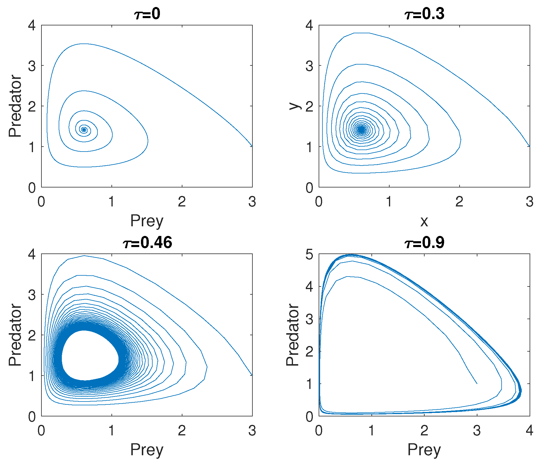
Figure 1 shows the phase portraits of the deterministic system given by Equation (1) for different values of the time delay $\tau$, and for the parameter values $r=0.8$, $K=5$, $\sigma =0.01$, $\beta =0.5$, and $a=0.3$ [17]. For these values, the interior equilibrium is $(x^{*},y^{*})=(0.6036,1.4153)$, ${\mathcal{R}}_0=8.2833$ and ${\mathcal{R}}_c=2.9881$. This corresponds to the case where $1<{\mathcal{R}}_c<{\mathcal{R}}_0$. As can be seen, there is a critical value of $\tau$, the system switches from a stable fixed point to a limit cycle.

Figure 1. Phase portraits of Model (1) at different time delays. $r=0.8,K=5,\sigma =0.01,\beta =0.5$, $a=0.3\Rightarrow {\tau }^{*}=0.46$, and $0\le t\le$ 10,000. $x\left(0\right)=3,y\left(0\right)=1$.

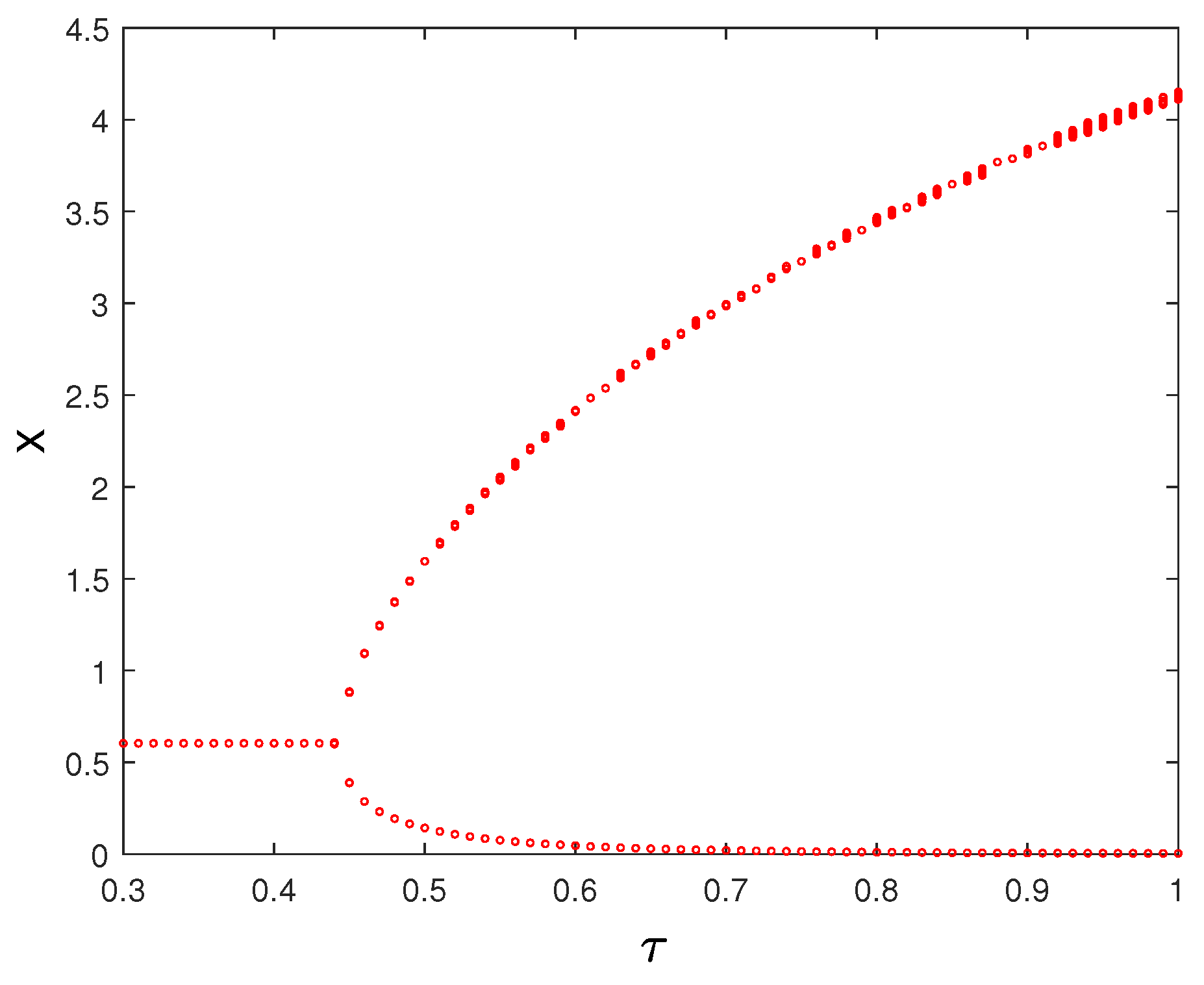
To better visualize these bifurcation patterns, we also plotted the bifurcation diagram with $\tau$ as a varying parameter (see Figure 2). According to our numerical results, the interior equilibrium is asymptotically stable for values of $\tau$ smaller than the bifurcation value ${\tau }^{+}=0.46$ at which the Hopf bifurcation occurs. At this critical value, the trajectories of the system slowly converge toward the limit cycle, while for values of $\tau$ larger than ${\tau }^{+}$, the behaviour of the system quickly collapses into the limit cycle (see Figure 1).

Figure 2. Hopf bifurcation diagram of the deterministic system (1) considering the time delay as a bifurcation parameter. For $\tau <0.46$, the interior equilibrium is asymptotically stable. For $\tau \ge 0.46$, an asymptotic limit cycle emerges.

3. Two Stochastic Models

In this section, we will construct two stochastic models and compare their asymptotic behaviour.

3.1. The First Stochastic Model (Model 1)

From a biological perspective, the inclusion of stochastic perturbations in the deterministic predator–prey model (1) allows for a more realistic interpretation of the system. The simplest way to do this is to add a white noise that is proportional to $x\left(t\right)$ and $y\left(t\right)$, leading to the following SDDE:

$$\left\{\begin{array}{c}dx\left(t\right)=\left[rx\left(t\right)\left(1-{\displaystyle \frac{x\left(t\right)}{K}}\right)-{\displaystyle \frac{\beta x\left(t\right)y(t-\tau )}{1+\sigma x\left(t\right)}}\right]dt+{\nu }_{1}x\left(t\right)d{W}_1\left(t\right),\hfill \\ dy\left(t\right)=\left[{\displaystyle \frac{\beta x\left(t\right)y(t-\tau )}{1+\sigma x\left(t\right)}}-ay\left(t\right)\right]dt+{\nu }_{2}y\left(t\right)d{W}_2\left(t\right),\hfill \end{array}\right.$$

(2)

where $W_1\left(t\right)$ and $W_2\left(t\right)$ denote two independent Brownian motions, and the positive constants ${\nu }_1$ and ${\nu }_2$ represent the intensity of the environmental white noises.

The numerical simulations use Milstein’s scheme for SDDEs, discussed in [18] or [14] (p. 137); actually, it is a simple adaptation of the method for an SDE of the same name which can be found in classical texts, e.g., [19,20], and more recently [21].

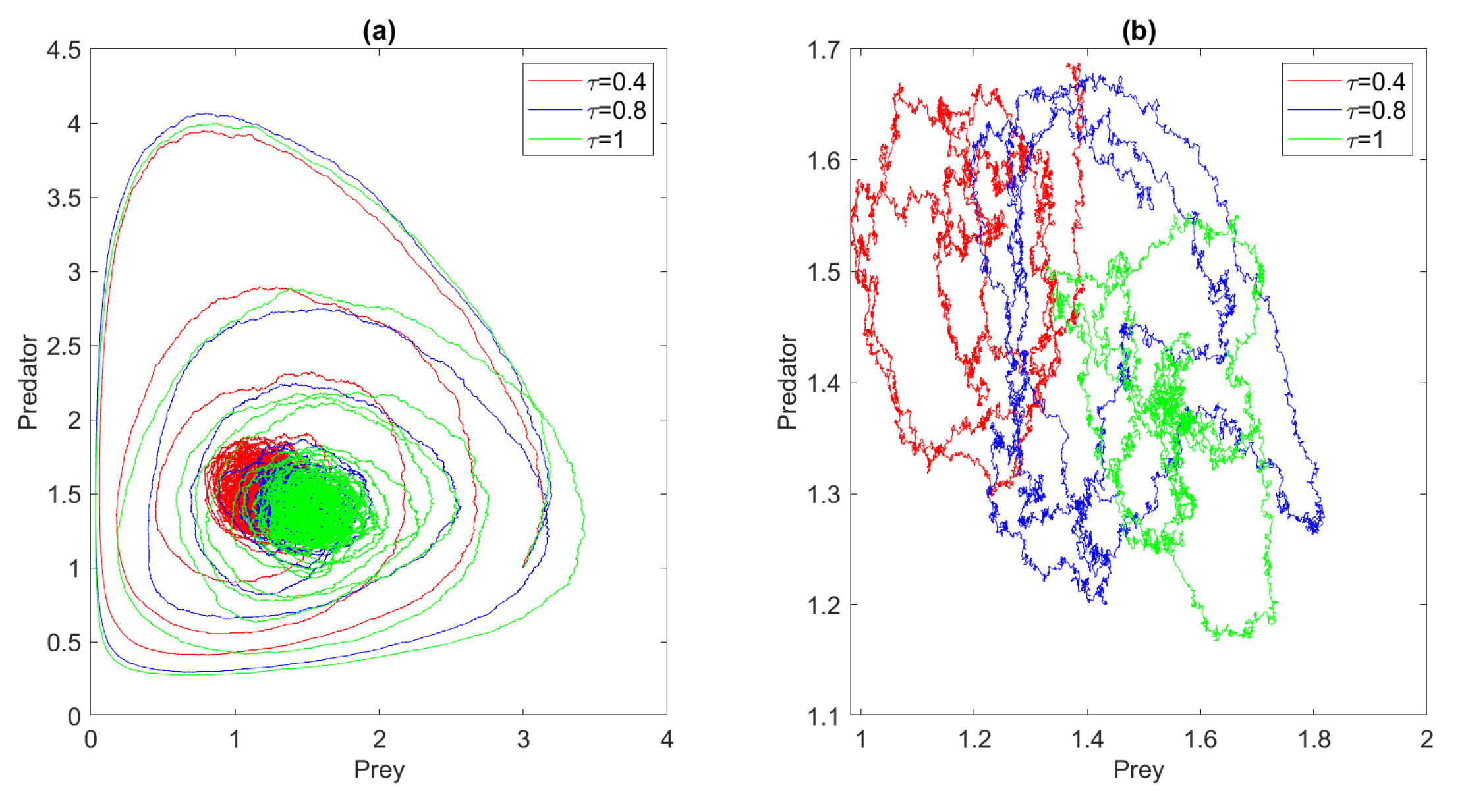
In Figure 3, we plotted the phase portraits the model for different values of the time delay $\tau$. The results were obtained from the stochastic data over 500 simulations and $0\le t\le 1500$. As you can see (panel (a)), for each value of $\tau$, the trajectories approach different fixed points, and no Hopf bifurcation is observed. In other words, the time delay moves the system to different regions of the state space where a particular stationary fixed point occurs.

Figure 3. (a) Phase portraits of the first stochastic model (model 1) for different values of the time delay $\tau$ for ${\nu }_1={\nu }_2=0.1$, $r=0.8$, $K=5$, $\sigma =1/3$, $\beta =0.5$, and $a=0.3$. The results were obtained from the stochastic data over 500 simulations and $0\le t\le 1500$. For the phase portrait in panel (b), we considered only the permanent regime.

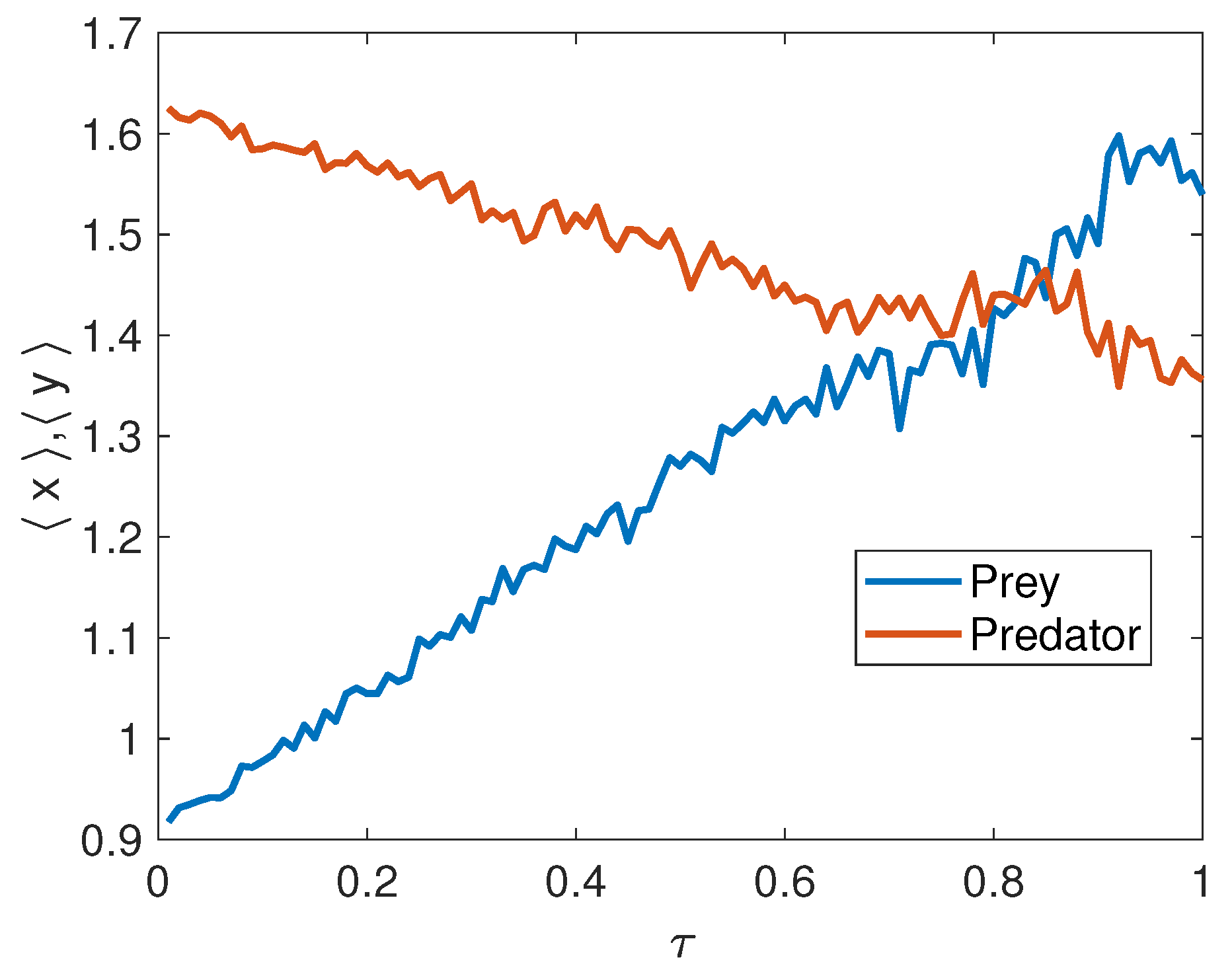
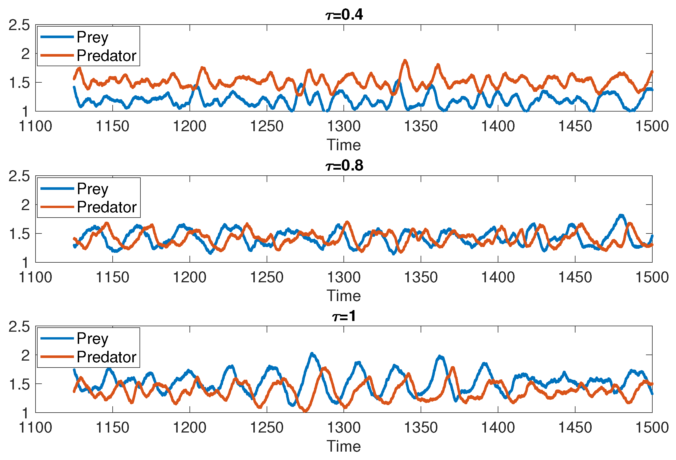
To better understand how the time delay affects the system dynamics, we also plotted the long-term average evolution of the steady-state equilibrium as a function of the time delay (see Figure 4). For each value of $\tau$, the trajectories were averaged over 500 runs and $0\le t\le 1500$. For values of $\tau$ less than ${\tau }^{**}=0.8$, the prey population is on average smaller than the predator population, while for values greater than ${\tau }^{**}$ the situation reverses and the predator population dominates the prey population. This value of ${\tau }^{**}$ is of course dependent on the capture rate $\sigma$, and increases with decreasing $\sigma$. At the critical value $\tau **$, the population sizes of prey and predators are equal on average (see Figure 5).

Figure 4. The first stochastic model (Model 1): The long-term average evolution of the stationary equilibrium as a function of the time delay. ${\nu }_1={\nu }_2=0.1$, $r=0.8$, $K=5$, $\sigma =1/3$, $\beta =0.5$, and $a=0.3$.

Figure 5. The first stochastic model (Model 1): Long-term trajectories of the model for different values of the time delay $\tau$ for ${\nu }_1={\nu }_2=0.1$, ${\nu }_1={\nu }_2=0.1$, $r=0.8$, $K=5$, $\sigma =1/3$, $\beta =0.5$, and $a=0.3$. The results were obtained from the stochastic data over 500 simulations and $0\le t\le 1500$.

3.2. The Second Stochastic Model (Model 2)

The second stochastic model that we will consider, which we could call the probabilistic model, is very similar to the ones analyzed in [22,23,24,25], assuming that the changes and their probabilities are those given in Table 1.

Table 1. Possible changes in $\mathbf{Z}={(X,Y)}^T$ and their probabilities.

Change	Probability
$\Delta {\mathbf{Z}}^{\left(1\right)}={(1,0)}^T$	$p_1=rx\left(t\right)\left(1-{\displaystyle \frac{x\left(t\right)}{K}}\right)\Delta t$
$\Delta {\mathbf{Z}}^{\left(2\right)}={(-1,0)}^T$	$p_2={\displaystyle \frac{\beta x\left(t\right)Y(t-\tau )}{1+\sigma x\left(t\right)}}\Delta t$
$\Delta {\mathbf{Z}}^{\left(3\right)}={(0,1)}^T$	$p_3={\displaystyle \frac{\beta x\left(t\right)Y(t-\tau )}{1+\sigma x\left(t\right)}}\Delta t$
$\Delta {\mathbf{Z}}^{\left(4\right)}={(0,-1)}^T$	$p_4=ay\left(t\right)\Delta t$

Fixing $\mathbf{Z}\left(t\right)$ at time t, we calculate the expected change for $\mathbf{Z}={(X,Y)}^T$

$$\mathrm{E}(\Delta \mathbf{Z})=\sum _{j=1}^4{p}_j\Delta {\mathbf{Z}}^{\left(j\right)}=\left(\begin{array}{c}rx\left(t\right)\left(1-{\displaystyle \frac{x\left(t\right)}{K}}\right)-{\displaystyle \frac{\beta x\left(t\right)y(t-\tau )}{1+\sigma x\left(t\right)}},\\ {\displaystyle \frac{\beta x\left(t\right)y(t-\tau )}{1+\sigma x\left(t\right)}}-ay\left(t\right),\end{array}\right)\Delta t,$$

(3)

and the covariance matrix

$$\mathrm{E}(\Delta \mathbf{Z}{(\Delta \mathbf{Z})}^T)=\sum _{j=1}^4{p}_j(\Delta {\mathbf{Z}}^{\left(j\right)}){(\Delta {\mathbf{Z}}^{\left(j\right)})}^T=\mathbf{D}(x,y)\Delta t,$$

(4)

where $\mathbf{D}(x,y)$ is the diffusion matrix

$$\begin{array}{c}\hfill \mathbf{D}=\left(\begin{array}{cc}rx\left(t\right)\left(1-{\displaystyle \frac{x\left(t\right)}{K}}\right)+{\displaystyle \frac{\beta x\left(t\right)y(t-\tau )}{1+\sigma x\left(t\right)}}& 0\\ 0& {\displaystyle \frac{\beta x\left(t\right)y(t-\tau )}{1+\sigma x\left(t\right)}}+ay\left(t\right)\end{array}\right),\end{array}$$

so we arrive at a stochastic differential system

$$\left\{\begin{array}{c}dx\left(t\right)=\left[rx\left(t\right)\left(1-{\displaystyle \frac{x\left(t\right)}{K}}\right)-{\displaystyle \frac{\beta x\left(t\right)Y(t-\tau )}{1+\sigma x\left(t\right)}}\right]dt\hfill \\ +\sqrt{rx\left(t\right)\left(1-{\displaystyle \frac{x\left(t\right)}{K}}\right)+{\displaystyle \frac{\beta x\left(t\right)y(t-\tau )}{1+\sigma x\left(t\right)}}}d{W}_1\left(t\right),\hfill \\ dy\left(t\right)=\left[{\displaystyle \frac{\beta x\left(t\right)y(t-\tau )}{1+\sigma x\left(t\right)}}-ay\left(t\right)\right]dt+\sqrt{{\displaystyle \frac{\beta x\left(t\right)y(t-\tau )}{1+\sigma x\left(t\right)}}+ay\left(t\right)}d{W}_2\left(t\right)\hfill \end{array}\right.$$

(5)

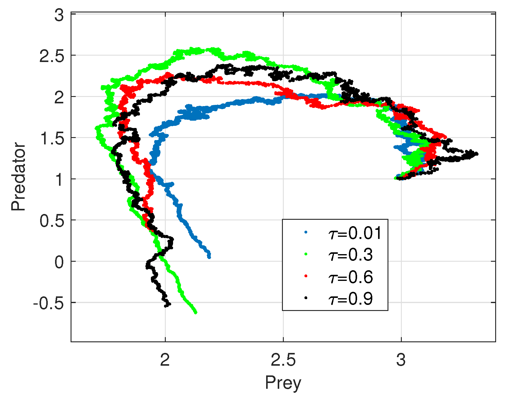
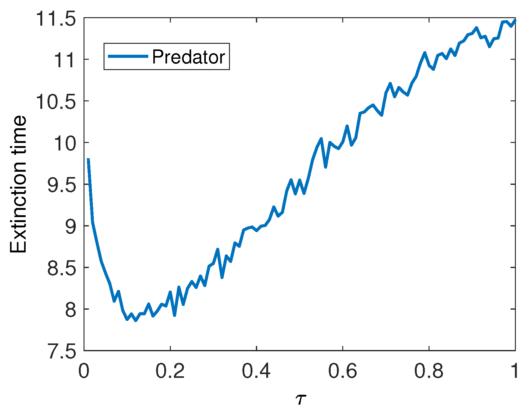
In Figure 6, we have plotted the phase portraits of Model 2 for different values of $\tau$, ranging from low to higher values. The results correspond to an average of 100 trials with initial values $x\left(0\right)=3,y\left(0\right)=1$, and $0\le t\le 9$. In this case, the predator population goes to extinction very quickly, and the time to extinction appears to increase with delay, showing a minimum for low values of $\tau$ (see Figure 7).

Figure 6. The second stochastic model (Model 2): Mean of 100 simulations. For $\tau =0.01$ in blue, $\tau =0.3$ in green, $\tau =0.6$ in red with $0\le t\le 9$, and $\tau =0.9$ in black with $0\le t\le 12$.

Figure 7. The second stochastic model (Model 2): Extinction time of the predator population as a function of time delay. The parameters of the model are $r=0.8$, $K=5$, $\sigma =1/3$, $\beta =0.5$, and $a=0.3$.

4. Conclusions

We have analysed the behaviour of two time-delayed stochastic differential systems for the prey–predator model and compared them with the corresponding deterministic system. The introduction of stochastic perturbations into these time-delayed models has a significant impact on population extinction and enriches the dynamics of the models. We found a significant difference between the deterministic system and the two classes of stochastic systems. Considering the time delay as a bifurcation parameter, the deterministic system exhibits a Hopf bifurcation leading to a critical ${\tau }^{+}$, from which the system transitions from the stable asymptotic fixed point to a stable limit cycle.

When the stochastic perturbation is modelled by simply adding a white noise to the deterministic components of the system (Model 1), the time delay appears to drive the system into different regions of state space where a particular stationary fixed point occurs, but no Hopf bifurcation is observed. Nevertheless, the population appears to be persistent for both the deterministic system and the stochastic Model 1. However, in contrast to what we observed previously, for the second stochastic system (Model 2) derived from a probabilistic approach, the system collapses rapidly and the population goes to extinction. This is consistent with previous work supporting the fact that the nature of the stochastic system has a significant impact on the asymptotic behaviour of the population, and environmental noise can cause the solution of the stochastic system to be extinct [23]. On the other hand, this shows that reliable population projections require modelling of both the environment and demographic stochasticity, and that uncertainty must be taken into account when estimating model parameters [26].

References

- Brockman, J. The Third Culture: Beyond the Scientific Revolution; Simon and Shuster: New York, NY, USA, 1995. [Google Scholar]
- May, R. Stability and Complexity in Model Ecosystems; Cambridge University Press: Cambridge, UK, 1973. [Google Scholar]
- Murray, J. Mathematical Biology I: An Introduction, 3rd ed.; Springer: Berlin/Heidelberg, Germany, 2002. [Google Scholar]
- Simmons, G. Differential Equations with Applications and Historical Notes; McGraw-Hill International Editions: New York, NY, USA, 1972. [Google Scholar]
- Boyce, W.; Diprima, R. Elementary Differential Equations and Boundary Value Problems, 4th ed.; John Wiley and Sons: Hoboken, NJ, USA, 1986. [Google Scholar]
- de Vries, G.; Hillen, T.; Lewis, M.; Müller, J.; Schönfisch, B. A Course in Mathematical Biology; SIAM: Philadelphia, PA, USA, 2006. [Google Scholar]
- Neal, D. Introduction to Population Biology; Cambridge University Press: Cambridge, UK, 2004. [Google Scholar]
- Sharin, M. Exploration of Methematical Modles in Biology with MATLAB; Wiley: Hoboken, NJ, USA, 2014. [Google Scholar]
- Chou, C.; Friedman, A. Introduction to Mathematical Biology. Modeling, Analysis, and Simulations; Springer: Berlin/Heidelberg, Germany, 2016. [Google Scholar]
- Allen, L. An Introduction to Stochastic Processes with Applications to Biology; Person Prentice Hall: London, UK, 2003. [Google Scholar]
- Allen, E. Modeling with Itô Stochastic Differential Equations; Springer: Berlin/Heidelberg, Germany, 2007. [Google Scholar]
- Chasnov, J. Mathematical Biolgy; The Hong Kong Univeristy of Science and Technology: Hong Kong, China, 2009. [Google Scholar]
- Pardoux, E. Probabilistic Models of Population Evolution Scaling Limits, Genealogies and Interactions; Springer: Berlin/Heidelberg, Germany, 2016. [Google Scholar]
- Rihan, F. Delay Differential Equaitons and Applications to Biology; Springer: Berlin/Heidelberg, Germany, 2021. [Google Scholar]
- Sunthrayuth, P.; Ullah, R.; Khan, A.; Shah, R.; Jeevan Kafle, I.M.; Jarad, F. Numerical Analysis of the Fractional-Order Nonlinear System of Volterra Integro-Differential Equations. J. Funct. Spaces 2021, 2021, 1537958. [Google Scholar] [CrossRef]
- Freedman, H.I. Deterministic mathematical models in population ecology. Can. J. Stat. 1980, 10, 315. [Google Scholar]
- Shampine, L.; Gladwell, I.; Thompson, S. Solving ODEs with MATLAB; Cambridge University Press: Cambridge, UK, 2003. [Google Scholar]
- Hofmann, N.; Müller-Gronbach, T. A modified Milstein scheme for approximation of stochastic delay differential equations with constant time lag. J. Comput. Appl. Mathet. 2006, 197, 89–121. [Google Scholar] [CrossRef]
- Higham, D. An Algorithmic Introduction to Numerical Simulation of Stochastic Differential Equations. SIAM Rev. 2001, 43, 525–546. [Google Scholar] [CrossRef]
- Kloeden, P.; Platen, E. Numerical Solution of Stochastic Differential Equations; Cambridge University Press: Cambridge, UK, 1998. [Google Scholar]
- Higham, D.; Kloeden, E. An Introduction to the Numerical Simulation of Stochastic Differential Equations; SIAM: Philadelphia, PA, USA, 2021. [Google Scholar]
- de la Hoz, F.; Vadillo, F. A mean extinction-time estimate for a stochastic Lotka-Volterra predator-prey model. Appl. Math. Comput. 2012, 219, 170–179. [Google Scholar] [CrossRef]
- Vadillo, F. Comparing stochastic Lotka-Volterra predator-prey models. Appl. Math. Comput. 2019, 360, 181–189. [Google Scholar] [CrossRef]
- de la Hoz, F.; Doubova, A.; Vadillo, F. Persistence-time Estimation for some Stochastic SIS Epidemic Models. Discret. Countinous Dyn. Syst. Ser. B 2015, 20, 2933–2947. [Google Scholar] [CrossRef]
- Moujahid, A.; Vadillo, F. Modeling and Calibration for Stochastic Differential Models. Fractal Fract. 2022, 6, 707. [Google Scholar] [CrossRef]
- Engen, S.; Saether, B.E.; Moller, A.P. Stochastic Population Dynamics and Time to Extinction of a Declining Population of Barn Swallows. J. Anim. Ecol. 2001, 70, 789–797. [Google Scholar] [CrossRef]
Disclaimer/Publisher’s Note: The statements, opinions and data contained in all publications are solely those of the individual author(s) and contributor(s) and not of MDPI and/or the editor(s). MDPI and/or the editor(s) disclaim responsibility for any injury to people or property resulting from any ideas, methods, instructions or products referred to in the content. |
© 2023 by the authors. Licensee MDPI, Basel, Switzerland. This article is an open access article distributed under the terms and conditions of the Creative Commons Attribution (CC BY) license (https://creativecommons.org/licenses/by/4.0/).