Abstract
In bridge health monitoring, in order to closely monitor the structural state changes of the bridge under heavy traffic load and other harsh environments, the monitoring system is required to give the change process of structural modal parameters. Due to the symmetric variables of bridge monitoring during operation, the evaluation needs to be completed by the recursive identification of modal parameters based on environmental excitation, especially the recursive recognition of the random subspace method with high recognition accuracy. We have studied the recursive identification methods of covariance-driven and data-driven random subspace categories respectively, established the corresponding recursive format, and used the model structure of the ASCE structural health monitoring benchmark problem as a numerical example to verify the reliability of the proposed method. First, based on the similar interference environment of the observation data at the same time, a reference point covariance-driven random subspace recursive algorithm (IV-RSSI/Cov) based on the auxiliary variable projection approximation tracking (IV-PAST) algorithm is established. The recursive format of the system matrix and modal parameters is obtained. Based on Givens rotation, the rank-2 update form of the row space projection matrix is established, and the recursive format of the data-driven recursive random subspace method (RSSI/Data) under the PAST algorithm is obtained. Then, based on the benchmark problem of ASCE-SHM, the response of the model structure under environmental excitation is numerically simulated, the frequency, damping ratio and vibration mode of the structure are recursively tracked, and their reliability and shortcomings are studied. After improving the recursive method, the frequency tracking accuracy has been improved, with a maximum accuracy of 99.8%.
1. Introduction
Bridge Health Monitoring (BHM) is just one specific application of Structural Health Monitoring (SHM) in the field of bridge engineering, and the two have the same connotation. Bao et al. [1] describe SHM as structural health monitoring as the process of implementing damage diagnosis strategies for aeronautical, civil and mechanical engineering structures, clearly stating the main task of damage diagnosis in SHM. Early diagnosis of structural damage is one of the core tasks of the health monitoring system.
Damage to a structure is reflected as changes in material and geometric properties, including boundary constraints and connection conditions. The goal of damage diagnosis is to try to gradually answer the following five progressively deeper questions [2]: (1) whether there is damage; (2) the Location of the damage; (3) the type of damage; (4) the extent of the damage; (5) Structural remaining life prediction (prognosis).
It is fully understood that for modal parameter identification of symmetric variables, the use of the recursive stochastic subspace method is very effective. From the perspective of bridge maintenance and management, if the degree of damage reaches a certain limit, the predicted result of the remaining life of the structure will not meet the requirements (or understood as the current state assessment of the structure does not meet the requirements), it is necessary to take certain maintenance measures to repair and strengthen the structure (that is, damage control), and then the reliability of the structure is improved, the predicted remaining life (or structural state assessment) will meet the requirements again, and then continue to bear possible damage in operation.
It can be seen that bridge maintenance based on a health monitoring system is a dynamic cycle process including online monitoring, damage diagnosis, structural assessment, and decision-making. Compared with the traditional detection and maintenance method, the first three links have new theoretical connotations, which makes bridge maintenance more scientific.
The online monitoring link of the bridge should involve more hardware development, and the current development of related technologies in this area is very rapid [3,4,5,6], the introduction of new sensing elements in other industries such as aviation, machinery and other fields, as well as new sensing and transmission ideas (such as various intelligent sensors, distributed sensors, wireless transmission, etc.), will greatly promote the research of subsequent links. Due to the convenience, fast and effective characteristics of vibration monitoring (acceleration response measurement not only does not require an absolute reference point, but also uses environmental excitation conveniently and cheaply), the vibration-based bridge health monitoring theory has been extensively and deeply studied [7].
In the damage diagnosis link, according to whether the diagnostic process needs to establish a structural finite element model, it can be divided into two categories: model-based (such as model modification method, etc.) and signal-based (such as damage index method).
The signal-based damage index method is directly extracting dynamic characteristics (or dynamic fingerprints) that can reflect structural damage based on monitoring signals, and directly determine whether the damage is damaged or not according to their changes. These dynamic characteristics include structural frequency [8,9,10], structural mode shape (including modal guarantee criterion MAC and coordinate mode guarantee criterion COMAC [11,12], strain mode or curvature mode [13,14,15,16], modal flexibility [17] (including damage localization vector DLV method [18], uniform load flexural surface method [19,20]), modal strain energy [21,22,23,24,25], etc. Farrar’s I-40 bridge-based damage test study clarifies that although various damage index methods can correctly diagnose the most severe damage conditions, the effect is not satisfactory when the damage is mild [26,27]. Several current studies have demonstrated that environmental conditions, particularly changes in temperature, interfere significantly with injury diagnosis [28,29,30,31]. In short, although the damage index method does not require detailed design information of the structure, it can generally only answer the first-level question of damage diagnosis, that is, to determine whether the damage occurs, and it is difficult to give damage localization and quantitative answers.
The model modification method integrates the two complementary technologies of structural finite element analysis and dynamic monitoring, which is more conducive to answering more in-depth questions in diagnosis, especially when the initial state information such as design documents and bridge formation tests of new bridges is easier to obtain. After nearly half a century of development, the model modification theory has been relatively mature [32], and has achieved many successful applications in machinery, aviation and other fields.
Condition assessment techniques based on health monitoring are a more in-depth issue. Reasonable structural state definition, scientific evaluation system and methods are all key issues worthy of studying [33,34,35,36,37,38,39]. At present, in general, research in this area mainly focuses on how to use monitoring and processing information to extend the use of structural reliability methods and the use of traditional structural assessment methods, and there has been some progress in some aspects.
In general, in multiple-input multiple-output (MIMO) subspace recognition applications, less attention is paid to the automation of the recognition process because the total recognition workload is not large, and the final recognition results are often selected manually. In the field of SHM, such as bridge health monitoring, huge amounts of monitoring data are often generated, and the huge workload would prevent the achievement of the monitoring goals if this approach is adopted, so they need to be improved to achieve automatic modal identification (AMI) without human intervention. In addition, automatic recognition not only saves a lot of tedious human effort due to its automation, but also overcomes the inevitable subjectivity of human intervention and the inability to base final inferences on comprehensive and complex comparisons by introducing scientific discriminant methods. Finally, the study of automatic modal recognition can also contribute to the diffusion of modal analysis tools to the general user community.
The CMIF method (or FDD method), SSI, and PolyMAX are three methods that have been widely used in bridge health monitoring for operational modal analysis under environmental stimuli [40], and the idea of implementing automatic modal parameter identification in various methods is mainly to simulate the “logical” process during the human intervention. The CMIF method is used to automatically identify the modal parameters of the Hong Kong Tingjiu cable-stayed bridge for one year, but the author does not elaborate on the specific implementation process of the method [41]. The modal consistency index (essentially the modal guarantee criterion MAC value) is proposed to be defined, the MAC value of the singular vector corresponding to the point near the peak of the maximum singular value discrete curve, and the MAC value of the singular vector corresponding to the peak point is greater than the predetermined critical value. Then the point belongs to the homemade region, otherwise, it belongs to the noise mode, and then complete the modal parameter identification according to the idea of FDD, the key of the method is to determine the appropriate critical MAC value [42]. Magalhães [43] adopts a similar method, and the corresponding feature of the peak is judged to be the true mode by the criterion that there are homemade regions on both sides of a peak on the maximum singular value discrete curve and the number of frequency points belonging to the homemade is greater than the number of critical points, and the paper claims to receive good results. Mcmillan [44] proposes to first determine the corresponding frequency bandwidth of each mode (decompose the singular values of the intersectoral matrix formed after data grouping, draw the average MAC-frequency curve between the vectors corresponding to the largest singular value of each group. The frequency width of the average MAC value greater than a predetermined value is the frequency bandwidth of the mode), and then identify the modal parameters through the inverse Fourier transform according to the idea of FDD. Yue [45] designed a threshold value to present the damage index to obtain information regarding the existence of structural damage. The threshold can be used to distinguish a damaged state from an undamaged state.
The recognition automation of SSI and PolyMAX methods is carried out on the basis of stable graphs, which essentially use stable maps to automatically eliminate false modes. Rainieri [46] proposes the simplest automatic identification method, which determines whether the modal estimation of each order of the system is a stable point, and takes the number of stable points to reach an artificially specified critical value as the judgment condition for the true mode after determining whether the modal estimation of each order of the system is a stable point. Deraemaeker [47] defines the i-th order “modal transformation norm” (MTN) based on the modal decomposition of the positive value spectrum (Fourier transform of the positive time-delay cross-correlation function) of the response power spectrum, which describes the importance of the i-th modal component in the spectrum. Select the structure order, calculate the MTN of each order mode and arrange it in descending order, use the identification results of the previous one period as a reference, compare the distance between the mode arranged in this period and the mode of each order in the previous one period, and determine that the nearest mode is the estimated result of the mode in this period.
Another type of automatic recognition method based on stable graphs is clustering. Magalhães [48] defines the distance between stable points as the sum of the relative frequency difference and (1-MAC), and the distance between classes is defined as the shortest distance between any two points between the two classes, and then the system clustering algorithm is applied to condense the stable points, and finally, the class containing the number of stable points greater than a certain predetermined value is the real modal class. The fuzzy C-means clustering method is applied to realize the automatic identification of the covariance-driven random subspace method [49]. In addition, some single-modal criteria such as modal phase collinearity (MPC) and modal mean phase deviation (MPD) are used to eliminate spurious modes.
2. Automatic Modal Identification Based on the RSSI-Cov/Ref Algorithms
This section proposes automatic modal parameter identification based on the SSI and DBSCAN algorithms. The identification process is as follows.
(1) Step 1: Determine the initial period T0 and sampling data length N0, select the number of observation data matrix row blocks i, the number of auxiliary variable channels r, the delay length h and the number of row blocks m, and set the corresponding Hankel matrix and according to the new weighting mechanism.
(2) Step 2: The covariance matrix is decomposed by SVD.
(3) Step 3: Obtain the extended observable matrix under the new mechanism.
(4) Step 4: The system matrices A and C are obtained.
(5) Step 5: The structural modal parameters and in the initial period are obtained.
(6) Step 6: Assign initial values W(0), P(0) to recursive variables W, P.
(7) Step 7: Set the block observation vector and auxiliary variable block column vector containing the latest sampling time data according to the formula.
(8) Step 8: Recursive update W (t), P (t).
(9) Step 9: Solve system matrices A and C.
(10) Step 10: Obtain the structural modal parameter and at the current time t.
(11) Step 11: t = t + 1, repeat the solution process in steps (7) to (10) until the end of the data period.
For the recursive identification of the above auxiliary variables, it is worth pointing out that when the process and measurement noise do not meet the broadband white noise assumption, such as band-pass white noise, as long as the autocorrelation length of the noise is less than the delay length hΔt of the auxiliary variable (that is, it is less than the autocorrelation length of the output measurement), the symmetric modal parameters can be correctly identified, and when h = 1, it will degenerate into the classical covariance driven random subspace identification.
2.1. Hankel Matrix Weighting Mechanism
In both offline random subspace modal identification and online identification, the covariance Toeplitz matrix can be obtained by sorting the measured output of each channel into the following Hankel matrix (assuming the number of sampling points in the period is N0), and then the product of its block matrix.
In the above formula, the three numbers in the and subscripts correspond to the subscripts of the observation data column vector of the upper left element of the matrix, namely the observation discrete time series number, the number of row blocks of the matrix and the observation time series number of the observation data of the lower right element.
The starting point of the new weighting mechanism is that when processing the data of any time period, the weighting value of the most recent observation data is taken as 1, and the observation data is multiplied by the weighting coefficient of for each forward sampling period of 1 unit. So, the weighted Hankel matrix of the initial period is:
Although the form of the above formula is the same as that of the old update formula, because the new block column vector is set according to the formula and the formula, the data of the entire period can meet the principle of weighting according to the different distance from the “current time”, and ensure that the weight of the same observation vector y is equal when it appears in different positions.
2.2. Auxiliary Variable Projection Approximation Subspace Tracking Algorithm (IV-PAST)
The recursive calculation needs to first determine the initial values W(0) and P(0). For W(0), there are two ways to assign the initial value: one is to perform offline identification in the initial period of data to obtain the left singular vector Ur group integration W(0) of the covariance matrix, and the other is to take any full-rank matrix such as the formula as the initial value. can also be used as the initial value. This simple assignment only affects the modal tracking results in a short time after the initial period, and has no effect on the stability of the tracking results in the later period of the algorithm.
where is the identity matrix of order r’. The auxiliary variables are discussed as follows. (1) Selection of auxiliary variable : it should be orthogonal to the noise in the random measurement signal z(t). Generally, the measurement signal after a certain time delay can be taken or the signal can be grouped, with some channels as the measurement signal and some channels as the auxiliary variable signal. (2) The length of the auxiliary variable : there is no limit to the length. When the value is equal to the length of the signal z(t), the recursive formula can also be simplified, but in theory, the greater the length of the auxiliary variable, the better the tracking accuracy. When the auxiliary variable is taken as h(t), the method will degenerate into Yang’s projection approximation algorithm (PAST), and then the formula of the signal subspace basis vector result will degenerate into the formula.
2.3. RSSI/DATA Algorithm
The data-driven random subspace method refers to the projection of the “future” output data Hankel matrix row space to the “past” output data Hankel matrix row space to complete data compression without traditional covariance calculation, and the symmetric system matrix will finally be obtained from the projection result. Since the projection matrix is obtained by QR decomposition, and the extended observable matrix Oi is calculated by SVD decomposition, it is necessary to update the QR decomposition and then introduce subspace tracking technology to obtain Oi, then the tracking modal parameters can be recursively calculated.
In the initial period T0, in the offline data-driven recognition algorithm, the row space of the “future” output data Hankel matrix is projected to the row space of the “past” output Hankel matrix . The projection result is obtained by the following QR decomposition:
The sequence product P(N0) of the Givens rotation matrix is introduced (It is also an orthogonal matrix, there is PPT = I), so that it meets
The QR decomposition of in the formula above should be recursively solved for modal parameter tracking. However, the formula and subsequent solutions that the information of the Q matrix is not required for modal tracking. In fact, only the solution R(N0 + 1) can be recursively solved, which can be obtained from the formula.
It can be seen from the recognition theoretical formula that the extended observable matrix Oi can be obtained from the SVD decomposition. Since the eigenvector in the eigenvalue decomposition (EVD) is the same as the left singular vector of the SVD decomposition, Oi can also be obtained from the EVD decomposition of the “correlation” matrix of R(N0 + 1) on the left of the formula.
3. Numerical Studies
3.1. ASCE-SHM Symmetric Model Structure
The symmetric frame model of the ASCE benchmark problem is studied to test the methods developed in this paper, as Figure 1 [17]. This numerical example adopts a scaled model of a bridge steel structure frame. The frame is made of hot-rolled 300W grade steel (nominal yield strength 300 Mpa), and the cross-section is specially designed for testing. In order to simplify the research, this paper treats the structure as a simplified shear beam model, that is, a 4-degree-of-freedom structure, and the simplified model is shown in Figure 2, so the cross-sectional characteristics of the beams, columns and supporting components of the structure will not be described here. The qualities of each layer of the 4-degree-of-freedom finite element simplified model of the frame structure are m1 = 3452.4 kg, m2 = m3 = 2652.4 kg, m4 = 1809.9 kg. The interlayer stiffness is k1 = k2 = k3 = k4 = 67.9 MN/m; The damping matrix is 1%, 0.7%, 0.8%, 0.9% calculated according to Rayleigh damping, and the damping ratio of each order is set respectively, and the coefficients corresponding to the mass matrix and the stiffness matrix are 1 s−1 and 5 × 10⁻⁵ s, and the theoretical frequencies of the structure are 9.41 Hz, 25.54 Hz, 38.66 Hz and 48.01 Hz, respectively.
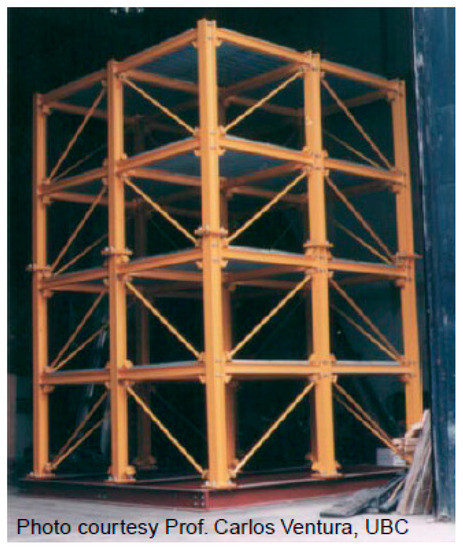
Figure 1.
ASCE-SHM benchmark problem research structure prototype.
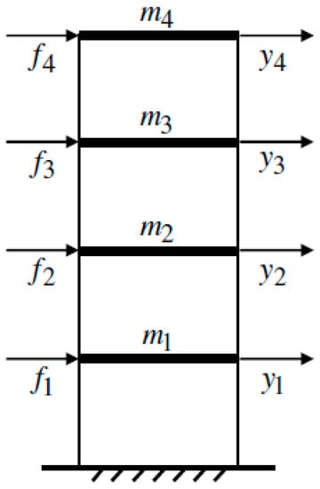
Figure 2.
Simplified model, i.e., 4 degrees of freedom shear beam structure.
3.2. RSSI/COV Recursive Tracking
The simulation applies excitation Fi, i = 1…4, at each floor slab of the structure, the sampling frequency is 250 Hz, the sampling time length is, and the following three working conditions are considered:
(1) The excitation Fi and measurement noise vi are independent broadband Gaussian white noise, and the structural stiffness K, mass M and damping matrix C remain unchanged, that is, the structural modal characteristics remain unchanged.
(2) The excitation Fi and measurement noise vi is changed to narrowband independent Gaussian white noise within 50, and the structural characteristic matrices K, M and C remain unchanged.
(3) The excitation Fi and measurement noise vi is independent wideband white Gaussian noise, but the interlayer stiffness K1 of the first layer of the structure is linearly attenuated to 0.5 K1 between the 10th and 15th seconds (the frequency fi of each order of the structure will also be linearly attenuated during this period), and the mass matrix M and the damping ratio of the structure remain unchanged (the damping matrix C must change accordingly according to Rayleigh’s damping theory).
First, you need to simulate the source data (i.e., acceleration “measurement” data) needed to obtain the tracking algorithm, and you need to solve the structural response of the simplified model at different inputs. For working case 1 and working case 2, because the structural characteristic matrix is invariant in the dynamic response problem of linear time-invariant (LTI) system, there are various methods such as model superposition method, stepwise integration method, state space method, etc. can be used; For working case 3, the modal superposition method is no longer applicable because the structural stiffness matrix and damping matrix C change during the time period, that is, the response problem of the linear parameter change (LPV) instant-changing structure. If it is assumed that the structural characteristics only change at the sampling point moment, and the “zero-order hold” assumption is satisfied when it does not change during the sampling interval, the following two methods can be used to approximate the calculation.
For the state space method, because the state transition matrix of the time-varying structure is difficult to obtain, it is approximated by the assumption of “zero-order retention” to apply it to the current sampling period, first the state variable and output variable at the endpoint of the sampling interval are obtained by recursion of the state equation of the sampling interval according to the state equation recursion method of the time-invariant structure, and then the structural characteristic matrix is updated, and then the next 1 sampling interval is recursively calculated according to the new state equation until the entire period.
For the stepwise integration method, first, discretize the time of the vibration differential equation, and only require the structure to be accurately satisfied at the discrete time series point, then assume that the structural characteristic matrix in the sampling interval is unchanged, that is, the time-invariant structure in the interval, assume the acceleration change law in the time period, and finally solve the motion-related quantity at the end moment of the sampling interval according to the motion law. If the method is used to solve (), it is an unconditional convergence algorithm.
In case 1, the white Gaussian noise excitation Fi, 5% rms measurement of white Gaussian noise v1, and the front 10 s history waveform and normalized autocorrelation function of the structural acceleration response y1 based on state-space recursion is shown in Figure 3. Since the excitation and noise both satisfy the wideband white noise assumption, the auxiliary variable delay h = 1 is taken, that is, the classical covariance-driven random subspace method is used for recursive identification.
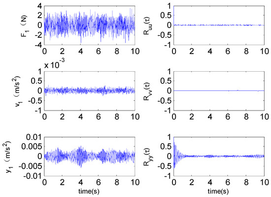
Figure 3.
Time history waveform and normalized autocorrelation function (τ > 0) for Gaussian white noise excitation force F1, measuring white noise v1 and acceleration response y1 in working condition 1.
Since there is no structural damage, a large amnesia factor can be taken, and in order to determine the number of rows and blocks i of formula 3 of the data matrix forming the covariance matrix, recursive identification is carried out in four cases of i = 10, 30, 50, 80 respectively (the first 3s of the data are used as the initial period, and the offline batch algorithm is applied to it, and U, after the decomposition of the covariance matrix SVD is used as the initial value W(0), P(0), and the obtained frequency and damping ratio results, are shown in Figure 4, Figure 5, Figure 6 and Figure 7 (“S.F.” Represents the true structural frequency, “S.D.R.” represents the true structural damping ratio).
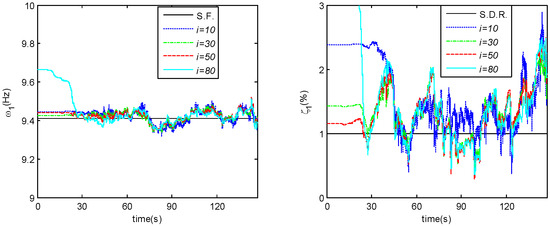
Figure 4.
Tracking results of the 1st frequency and damping ratio of working case 1 under a different number of rows and blocks.
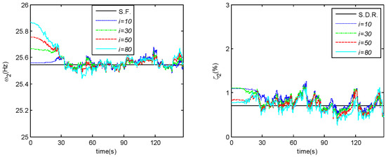
Figure 5.
Tracking results of second-order frequency and damping ratio of working condition 1 under a different number of rows and blocks.
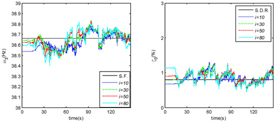
Figure 6.
Tracking results of the 3rd frequency and damping ratio of working case 1 under a different number of rows and blocks.
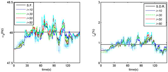
Figure 7.
Tracking results of the 4th frequency and damping ratio of working case 1 under a different number of rows and blocks.
From the identification results of frequency and damping ratio in Figure 2, Figure 3, Figure 4, Figure 5, Figure 6 and Figure 7, it can be seen that in the initial recursion period, such as within 30 s, there is a process of stabilizing to the real characteristics of the structure (but the difference percentage is still relatively small) under different row block number i. After the stabilization period such as 30 s, the recognition effect of different row block numbers for low-order modes is very small, and the difference is slightly larger in high-order modes, indicating that the number of different line blocks has a greater impact on the tracking of high-order frequencies than that of low-order modes. Overall, frequency tracking accuracy is good, as their percentage difference curve for true frequency is shown in Figure 3, with a value of about 0.2% and a maximum value of 0.59%.
Comprehensive Figure 8 can be seen that when the number of row blocks is 10, the recognition results of the frequency and damping of each order are quite different from the real value, but when the number of row blocks is higher than 10, that is, when they are taken as 30, 50 and 80, respectively, the difference percentage of each order decreases greatly and tends to be stable, which reflects the influence of the number of row blocks on the recognition results, indicating that the number of correlation submatrices needs to be determined high enough.
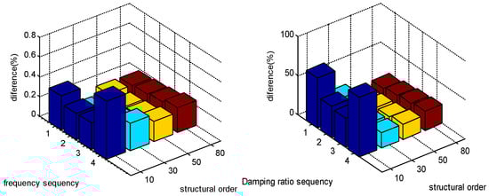
Figure 8.
Percentage difference in frequency and percentage difference in damping ratio for different number of row blocks i.
Figure 8 can also be seen that after taking a high enough number of row blocks, such as in the next three higher row block numbers, the frequency and damping ratio of each order mode The recognition value and the true value difference percentage are roughly the same, both of which are about 20%.
In addition, after determining the number of rows and blocks that is high enough, such as 30, 50, and 80, the percentage difference between the frequency and damping ratio of each order of the structure is about 10~20%, and the maximum difference percentage reaches 76% when i = 10. Based on the above observations, i = 50 was finally determined (this value was taken in subsequent studies in this paper).
The tracking results of the mode component ratio (the ratio of the 4th component of the j-mode shape to the other components ) at this time are shown in Figure 9. It can be seen from the figure that the components of each mode shape are better than the tracking results. The percentage difference between the component ratio and the true value in the period of 30–150 was 0.54%, 1.17%, 1.49% and 1.6%, respectively, and the average deviation was 1.2%.
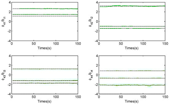
Figure 9.
Recursive tracking results of the mode shape component ratio of each order in working case 1 when the number of rows and blocks i = 50.
In the above recursion, the structure order r’ is taken as 4 (this value is also taken in the rest of this article), which is the true order of the structure. The determination of order is a common problem of all time-domain mode identification methods, which can theoretically be determined by the number of non-zero singular values or significant singular values decomposed by the SVD decomposition of the initial time period covariance matrix, as shown in Figure 10 of the first 20 singular values in this example, it can be seen that there is a significant difference between the 8th and 9th singular values, and the remaining singular values are basically zero, so it can be concluded that the state space order is 8. However, in practical applications, their differences may not be obvious, at this time you can also do a power spectrum analysis of the measurement channel, especially if the power spectrum of each channel is superimposed in the same diagram, then the number of their common peak is the number of structural orders, the result of this example is shown in Figure 10, it can be clearly seen that the structural order is 4.
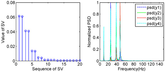
Figure 10.
Distribution of singular values (SV-singular values) and power spectrum for each measurement channel.
In case 2, both the excitation and measurement noises are narrowband white noise, and the power spectrum and autocorrelation function graphs for the excitation component u1 of Layer 1, the measurement noise (5% mean squared value) v1, and the Layer 1 measurement response y1 are shown in Figure 11. It can be seen from the figure that the excitation and noise have a certain autocorrelation length (about 50Δt), and it is advisable to use the delayed measurement output as an auxiliary variable for recursive identification, and the classical covariance random subspace method may not be ideal. Taking i = 50, β = 0.9995 the percentage intensity of the mean square value of the noise is 2%, and Figure 12 shows the comparison of the recursive recognition results of the structure frequency fi and damping ratio ξ in the case of classical SSI with delay h = 1 and auxiliary variable SSI at h = 20.
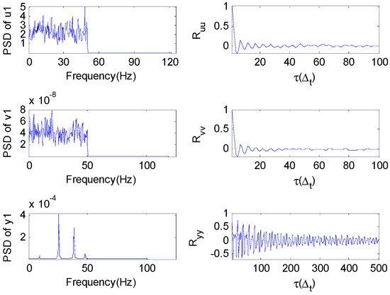
Figure 11.
Time limit for operating case 2 with excitation u1, noise v1, and power spectrum and autocorrelation function of measured output y1.
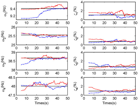
Figure 12.
Frequency and damping ratio results of recursive identification of h = 1 (blue line) and h = 20 (red line) in working condition 2.
It can be seen from the figure that the damping ratio of the two is similar, but the recognition effect is better when the frequency result h = 20, especially in the first-order mode. From 5 s to 50 s, the percentage difference between the frequency of each order and the true value was 0.73%, 0.17%, 0.28% and 0.20% when h = 1, and 0.39%, 0.15%, 0.10% and 0.26% at h = 20, respectively. The percentage difference between the damping ratio of each mode shape and the true value was 41.3%, 36.3%, 16.9% and 18.0% at h = 1, and 46.7%, 36.3%, 28.2% and 27.4% at h = 20, respectively. When h = 20, the comparison between the component ratio of each mode shape and the true value is shown in Figure 12, and the average percentage difference between the component ratio of each mode shape and the true value is 0.73%, 1.19%, 1.51% and 3.77%, respectively, which shows that the recursive recognition accuracy of mode shape is very high.
In case 3, the excitation and noise are both Gaussian white noise, which satisfies the noise assumption of subspace recognition, but the linear attenuation of the structural stiffness and the damping ratio of each mode remains unchanged, the state space model is a differential equation with a variation coefficient due to the change of stiffness matrix k and damping matrix c due to time, and its structure is a linear parameter change system. At this point, a “zero-order hold” can be taken after time discretization, and the state space method can be used to approximate the state and structure response within the sampling interval. When the linear attenuation reaches 50% of the original stiffness, the delay h = 1 is used, the measurement noise is 1% mean squared error, and the structural frequency results identified recursively with different forgetting factors are shown in Figure 13.
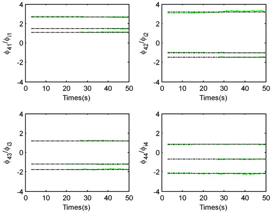
Figure 13.
Results of the component ratio of each mode shape identified by recursive identification of time delay h = 20 in working case 2.
It can be seen from Figure 14 that different forgetting factors have a great influence on the tracking accuracy of the region of decreasing stiffness, and the tracking is more accurate when the value is small in the low-order frequency of the structure, such as the 1st and 2nd order frequencies in this figure, this trend is clear, but it does not change much after β = 0.997; In the higher-order frequency tracking of the structure, the lower forgetting factor tends to cause greater tracking oscillations during the period when the structure frequency is unchanged, so it is necessary to balance these two considerations, and β = 0.997 is used in the subsequent parts of this example. Of course, it is more ideal to use a variable forgetting factor, a small forgetting factor in the stiffness change part, and a large forgetting factor in the stiffness unchanged part, but because the time point of the stiffness change cannot be known in advance during the recursion process, it is necessary to establish a suitable discriminant according to the recursion results to change the forgetting factor, which will be a big challenge.
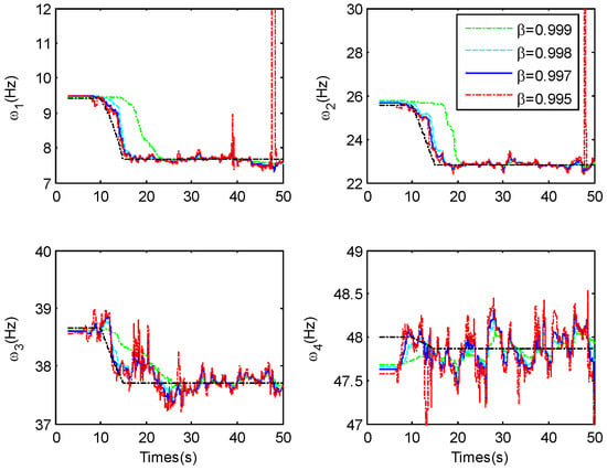
Figure 14.
Structural frequency recursion recognition results under different amnesia factor β under working condition 3.
After determining β = 0.997, the effects of different percent noise levels (i.e., noise mean square value and signal mean square value percentage NL) such as NL = 1%, 5%, 10% and 20% on the recursive results of structure frequency are shown in Figure 15. It can be seen from the figure that the difference between different noise levels for frequency regression recognition is small, and the robustness of the method is very good. When the percentage noise level of mean square value is NL = 20%, the first 3s period is used as the initial batch period, and the percentage difference between the frequency fi of each order structure and the true frequency is 1.45%, 0.68%, 0.39% and 0.31% in the 5s to 50 s period, respectively.
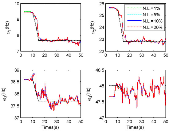
Figure 15.
Structural frequency recursive identification results at different noise levels under operating condition 3.
The tracking results of the structural damping ratio at the noise level NL = 20% are shown in Figure 16, and the percentage difference between the damping ratio and the true damping ratio of each order is 71.1%, 63.3%, 56.9% and 36.5% in the 5 s to 50 s period, respectively, and the damping ratio results at lower noise are shown in Figure 17, which shows that the oscillation of the damping ratio is directly related to the noise level as expected, which is likely to be caused by another reason such as the algorithm itself.
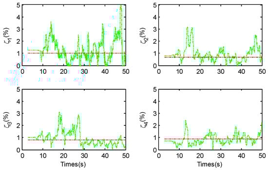
Figure 16.
Recursive identification results of structural damping ratio in working case 3 (β = 0.997, NL = 20%).
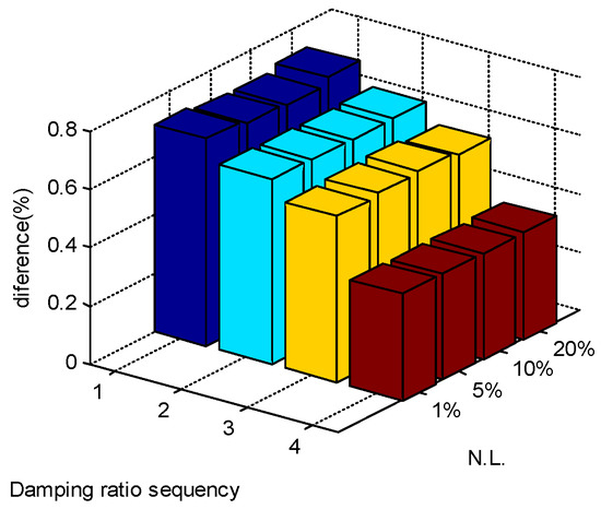
Figure 17.
Recursive identification results of structural damping ratio under different noise levels under working condition 3 (β = 0.997).
The tracking results of the mode shape component ratio of each order under the noise level NL = 20% are shown in Figure 18, and the average percentage difference from the true value is 4.57%, 4.04%, 3.55% and 5.10%, respectively, and the mode shape tracking accuracy is very ideal.
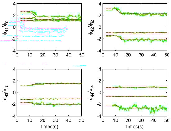
Figure 18.
Recursive identification results of mode component ratio in working case 3 (β = 0.997, NL = 20%).
3.3. RSSI/DATA Recursive Tracking
For data-driven stochastic subspace recursive identification, the numerical model of 4 degrees of freedom shear beam in the ASCE-SHM benchmark problem is still used to verify the recognition effect. The model incentive method is still to apply the excitation Fi at each floor slab, i = 1, … 4. The sampling frequency is 250 Hz, the sampling time length is 50 s, and the following two working conditions are considered:
(1) The excitation Fi and measured noise vi are independent broadband Gaussian white noise, and the structural stiffness K, mass M and damping matrix C remain unchanged, that is, the structural mode characteristics remain unchanged;
(2) The excitation Fi and measurement noise vi are independent wideband Gaussian white noise, but the interlayer stiffness k1 of the first layer of the structure is linearly attenuated to 0.5 k1 between the 10th and 15th seconds, and the mass matrix M and the structural damping ratio ξi remain unchanged.
For working case 1, according to the research results in the previous section, the initial 3 s data is used as the initial value matrix required for the initial period recognition of the formula (3.100), the forgetting factor β = 0.9995, the number of rows and blocks i of the data matrix is taken as 50, the percentage of the mean square value of the measured noise and signal is 10%, and the results of the frequency fi, damping ratio ξi and mode component ratio of each order of the structure after recursive identification are shown in Figure 19, Figure 20 and Figure 21, respectively.
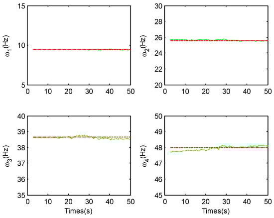
Figure 19.
Structural frequency recursion recognition results of working condition 1 (β = 0.9995, NL = 10%).
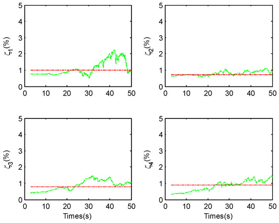
Figure 20.
Recursive identification results of structural damping ratio in working case 1 (β = 0.9995, NL = 10%).
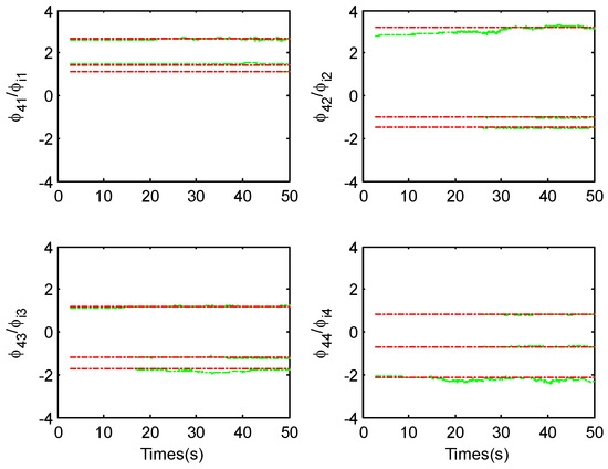
Figure 21.
Recursive identification results of mode component ratio in working case 1 (β = 0.9995, NL = 10%).
From 5 s to 50 s, the percentage difference between the frequency obtained by recursive identification and the true frequency was 0.41%, 0.35%, 0.18% and 0.24%, respectively. The percentage difference in the resulting damping ratio was 51.4%, 65.5%, 65.7% and 23.5%, respectively. The percentage difference of the component ratios of each mode shape was 1.91%, 1.49%, 2.11% and 1.95% on average. It can be seen that similar to the covariance-driven random subspace recursive recognition results, the accuracy of frequency and mode shape is good, but the recognition effect of the damping ratio is average.
In case 2, the interlaminar stiffness damage of the first layer of the model is 50%, and the forgetting factor has a significant impact on the recognition results, but its value range is not large, here β = 0.999, 0.9985, 0.998 and 0.9975 are taken, respectively, and the recognition results are shown in Figure 22. In the stiffness change segment, the recognition effect of different forgetting factors was more obvious, and the tracking was more sensitive and accurate at smaller values, but the forgetting factor no longer had a favorable effect on the recursive results after it dropped to 0.998, but on the contrary, it caused greater oscillations of the results, so β = 0.998 was taken in subsequent studies. Because β ≤ 1, its suitable value change range is not large, that is, the identification result is more sensitive to it, which will add certain difficulties to the adaptive study of forgetting factors.
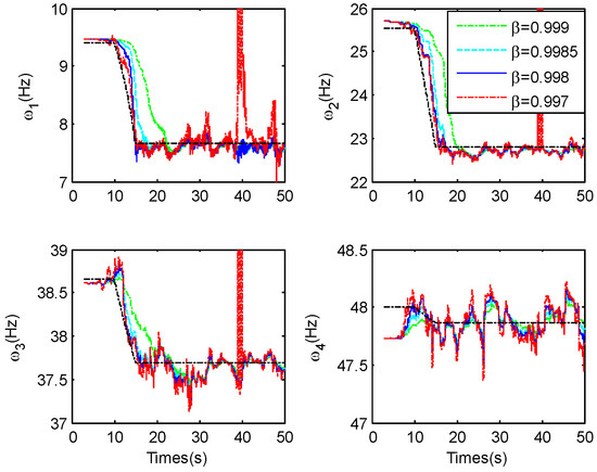
Figure 22.
Recursive recognition results of structural frequencies under different forgetting factors in case 1 (NL = 10%).
Under the determination of the forgetting factor of β = 0.998, the robustness of the identification results to the measured noise is studied, and the percentage of the mean square value of the measured noise and the signal is taken respectively, that is, the noise level (NL) is 5%, 10%, 20%, 50%, respectively, the recursive identification results of the structure frequency are shown in Figure 23, it can be seen that the degree of influence of noise on different modes is different, this calculation has a more obvious impact on the 1st order frequency results, and the robustness of the recursive recognition method is better overall, about 20% The identification results are more reliable under the mean square value noise. If the noise level is 20%, the percentage difference between the identified frequency result and the true frequency is 3.49%, 0.69%, 0.30% and 0.31%, respectively, within the 5 s to 50 s.
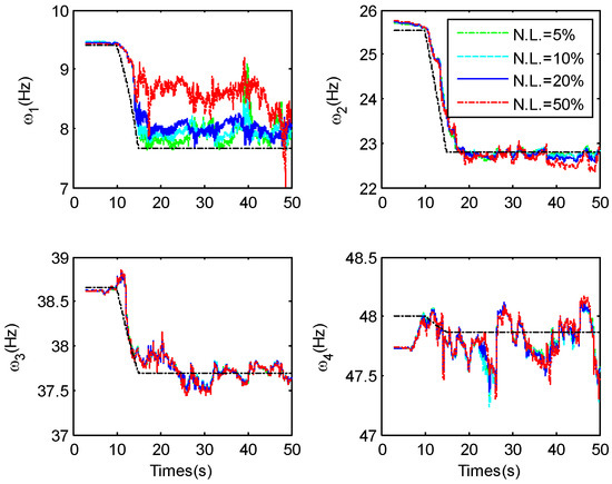
Figure 23.
Recursive identification results of structure frequencies under different noise levels under working condition 1 (β = 0.998).
At this time, the recursive recognition results of the structural damping ratio and mode shape component ratio are shown in Figure 24, Figure 25 and Figure 26, respectively. The damping ratio estimation is unreliable at 50% mean square noise, especially since the results of the 1st and 2nd orders are very different. The mode component ratio results were reliable, and the average percentage difference between the modal component ratio and the true value was 11.0%, 10.6%, 4.4% and 7.7% in the 5 s to 50 s, respectively.
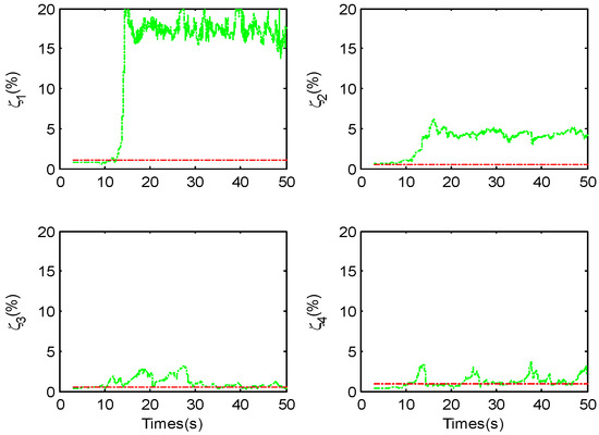
Figure 24.
Recursive identification results of structural damping ratio in operating condition 2 (damage 50%) (NL = 20%).
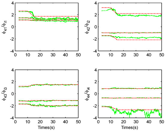
Figure 25.
Recursive recognition results of mode component ratio of structure in working case 2 (NL = 20%).
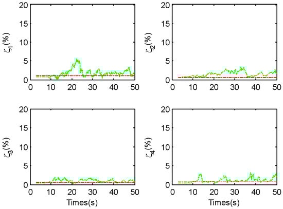
Figure 26.
Recursive identification results of damping ratio of structure in working condition 2 (when damage is 30%) (NL = 20%).
4. Conclusions
In order to track the structural modal properties in real time, this article focuses on the recursive recognition problem of the stochastic subspace method, and establishes covariance-driven and data-driven recursive implementation algorithms for symmetric variables:
(1) In the covariance-driven recursive identification, a new weighted form is first introduced to make the weights of the sampled data at each moment consistent everywhere in the algorithm, and then the auxiliary variable PAST algorithm is introduced to obtain the recursive formula of the extended observable matrix column space, so as to realize the recursive solution of modal characteristics. This method can complete the modal recursion identification problem under non-wideband white noise interference through the appropriate selection of auxiliary variables.
(2) In data-driven recursive recognition, the rank-2 update form of the row space projection matrix is first derived based on Givens rotation, and then the idea of the PAST algorithm is followed again, and the matrix inverse lemma is applied twice to obtain the recursive form of the extended observable matrix column space to complete the recursive modal recognition.
(3) Numerical examples show that the two recursive recognition methods mentioned in this paper have good tracking accuracy for frequency and mode shape. In the covariance-driven recursive identification, the percentage difference between the frequency recognition result and the true value at working condition 1~3 was 0.2~0.59%, 0.10~0.39% and 0.31~1.45%, respectively, and the different percentage of mode component ratio was 0.54~1.6%, 0.73~3.77% and 0.73~3.77%, respectively. In data-driven recursive recognition, the percentage difference between the frequency recognition result and the true value at working condition 1~2 is 0.18~0.41% and 0.30~3.49%, respectively, and the different percentage of mode component ratio is 1.91~2.11% and 4.4~11.0%, respectively.
(4) Numerical examples show that the tracking effect of the two methods on the damping ratio is inferior to the tracking results of frequency and mode shape. For example, in the covariance-driven random subspace recursive identification, the difference percentage of working condition 1 is about 20%, working condition 2 is about 20~40%, and working condition 3 reaches 30~70%; In data-driven recursive identification, the difference percentage of working case 1 is about 23.5~65.7%, and the damping ratio results of the 1st and 2nd mode modes in working condition 2 are unreliable, because this method cannot adapt to excessive damage degree, such as reducing the damage degree such as when the damage is changed to 30%, the difference percentage of damping percentage is about 47~89%, and there is no longer a serious deviation from the true value. Of course, the recognition results of the damping ratio are still not as ideal as the frequency and mode shape recognition results, which is due to the fact that the measurement noise has a relatively sensitive effect on the damping recognition results.
Author Contributions
Conceptualization, H.W.; methodology, H.W.; software, H.W.; validation, H.W.; formal analysis, Y.H.; investigation, Y.H.; resources, Y.H.; data curation, Y.H.; writing—original draft preparation, H.W. and Y.H.; writing—review and editing, H.W.; visualization, H.W.; supervision, Y.H.; project administration, Y.H.; funding acquisition, H.W. and Y.H. All authors have read and agreed to the published version of the manuscript.
Funding
This research was supported in part by Science and Technology Project of Education Department of Jiangxi Province under GJJ2200621, in part by National Natural Science Foundation of China under Grant 52165069, in part by Natural Science Foundation of Jiangxi Province under Grant 20224BAB214051, in part by National Natural Science Foundation of China under Grant 52005182, in part by Natural Science Foundation of Jiangxi Province under Grant 20202BABL214027.
Data Availability Statement
Not Applicable.
Acknowledgments
The authors thank all the reviewers who participated in the review.
Conflicts of Interest
The authors declare no conflict of interest.
References
- Bao, Y.; Chen, Z.; Wei, S.; Xu, Y.; Tang, Z.; Li, H. The State of the Art of Data Science and Engineering in Structural Health Monitoring. Engineering 2019, 5, 234–242. [Google Scholar] [CrossRef]
- Rytter, A. Vibrational Based Inspection of Civil Engineering Structures. Ph.D. Thesis, Aalborg University, Aalborg, Denmark, 1993. [Google Scholar]
- Boller, C.; Chang, F.; Fujino, Y. Encyclopedia of Structural Health Monitoring; John Wiley & Sons: Chichester, UK, 2009. [Google Scholar]
- Bao, Y.; Li, H.; Chen, Z.; Zhang, F.; Guo, A. Sparse l1 optimization-based identification approach for the distribution of moving heavy vehicle loads on cable-stayed bridges. Struct. Control Health Monit. 2016, 23, 144–155. [Google Scholar] [CrossRef]
- Li, H.; Ou, J.; Zhang, X.; Pei, M.; Li, N. Research and practice of health monitoring for long-span bridges in the mainland of China. Smart Struct. Syst. 2015, 15, 555–576. [Google Scholar] [CrossRef]
- Wang, H.; Tao, T.; Li, A.; Zhang, Y. Structural health monitoring system for Sutong Cable-stayed Bridge. Smart Struct. Syst. 2016, 18, 317–334. [Google Scholar] [CrossRef]
- Fan, W.; Lu, H.; Zhang, X.; Zhang, Y.; Zeng, R.; Liu, Q. Two-Degree-Of-Freedom Dynamic Model-Based Terminal Sliding Mode Control with Observer for Dual-Driving Feed Stage. Symmetry 2018, 10, 488. [Google Scholar] [CrossRef]
- Cawley, P.; Adams, R.D. The location of defects in structures from measurements of natural frequencies. J. Strain Anal. Eng. Des. 1979, 14, 49–57. [Google Scholar] [CrossRef]
- Mufti, A.A. Structural Health Monitoring of Innovative Canadian Civil Engineering Structures. Struct. Health Monit. 2002, 1, 89–103. [Google Scholar] [CrossRef]
- Yang, Y. Output-only modal identification by compressed sensing: Non-uniform low-rate random sampling. Mech. Syst. Signal Process. 2015, 56–57, 15–34. [Google Scholar] [CrossRef]
- Allemang, R.J. The modal assurance criterion-twenty years of use and abuse. Sound Vib. 2003, 37, 14–21. [Google Scholar]
- Lieven, N.A.; Ewins, D.J. Spatial Correlation of Mode Shapes: The Coordinate Modal Assurance Criterion (COMAC); Society of Experimental Mechanics: Bethel, Connecticut, 1988. [Google Scholar]
- Bao, Y.; Shi, Z.; Wang, X.; Li, H. Compressive sensing of wireless sensors based on group sparse optimization for structural health monitoring. Struct. Health Monit. 2017, 17, 823–836. [Google Scholar] [CrossRef]
- Zhou, X.-Q.; Xia, Y.; Weng, S. L1 regularization approach to structural damage detection using frequency data. Struct. Health Monit. 2015, 14, 571–582. [Google Scholar] [CrossRef]
- Ndambi, J.M.; Vantomme, J.; Harri, K. Damage assessment in reinforced concrete beams using eigenfrequencies and mode shape derivatives. Eng. Struct. 2002, 24, 501–515. [Google Scholar] [CrossRef]
- Zhang, C.D.; Xu, Y.L. Comparative studies on damage identification with Tikhonov regularization and sparse regularization. Struct. Control Health Monit. 2016, 23, 560–579. [Google Scholar] [CrossRef]
- Hou, R.; Xia, Y.; Bao, Y.; Zhou, X. Selection of regularization parameter for l1-regularized damage detection. J. Sound Vib. 2018, 423, 141–160. [Google Scholar] [CrossRef]
- Bernal, D. Load vectors for damage localization. J. Eng. Mech. 2002, 128, 7–14. [Google Scholar] [CrossRef]
- Yuen, K.-V.; Ortiz, G.A. Outlier detection and robust regression for correlated data. Comput. Methods Appl. Mech. Eng. 2017, 313, 632–646. [Google Scholar] [CrossRef]
- Wang, J.; Qiao, P. Improved damage detection for beam-type structures using a uniform load surface. Struct. Health Monit. 2007, 6, 99–110. [Google Scholar] [CrossRef]
- Wang, N.; Cao, G.; Yan, L.; Wang, L. Modeling and Control for a Multi-Rope Parallel Suspension Lifting System under Spatial Distributed Tensions and Multiple Constraints. Symmetry 2018, 10, 412. [Google Scholar] [CrossRef]
- Luo, Y.F.; Ye, Z.W.; Guo, X.N.; Qiang, X.H.; Chen, X.M. Data Missing Mechanism and Missing Data Real-Time Processing Methods in the Construction Monitoring of Steel Structures. Adv. Struct. Eng. 2015, 18, 585–601. [Google Scholar] [CrossRef]
- Shi, Z.; Law, S.; Zhang, L. Improved Damage Quantification from Elemental Modal Strain Energy Change. J. Eng. Mech. 2002, 128, 521–529. [Google Scholar] [CrossRef]
- James, H.S.; Wang, S.; Li, H. Cross-Modal strain energy method for estimating damage severity. J. Eng. Mech. 2006, 132, 429–437. [Google Scholar] [CrossRef]
- Yang, Y.; Nagarajaiah, S. Harnessing data structure for recovery of randomly missing structural vibration responses time history: Sparse representation versus low-rank structure. Mech. Syst. Signal Process. 2016, 74, 165–182. [Google Scholar] [CrossRef]
- Charles, R.F.A.D. Comparative study of damage identification algorithms applied to a bridge: I. Experiment. Smart Mater. Struct. 1998, 7, 704. [Google Scholar]
- Marasco, G.; Piana, G.; Chiaia, B.; Ventura, G. Genetic Algorithm Supported by Influence Lines and a Neural Network for Bridge Health Monitoring. J. Struct. Eng. 2022, 148, 04022123. [Google Scholar] [CrossRef]
- Duan, M.; Lu, H.; Zhang, X.; Zhang, Y.; Li, Z.; Liu, Q. Dynamic Modeling and Experiment Research on Twin Ball Screw Feed System Considering the Joint Stiffness. Symmetry 2018, 10, 686. [Google Scholar] [CrossRef]
- Zhang, Z.; Luo, Y. Restoring method for missing data of spatial structural stress monitoring based on correlation. Mech. Syst. Signal Process. 2017, 91, 266–277. [Google Scholar] [CrossRef]
- Chen, Z.; Bao, Y.; Li, H.; Spencer, B.F., Jr. A novel distribution regression approach for data loss compensation in structural health monitoring. Struct. Health Monit. 2017, 17, 1473–1490. [Google Scholar] [CrossRef]
- Sohn, H. Effects of environmental and operational variability on structural health monitoring. Philos. Trans. R. Soc. Math. Phys. Eng. Sci. 2007, 365, 539–560. [Google Scholar] [CrossRef]
- Friswell, M.I.; Mottershead, J.E. Finite Element Model Updating in Structural Dynamics; Kluwer Academic Publishers: Dordrecht, The Netherlands, 1995. [Google Scholar]
- Frangopol, D.; Strauss, A.; Kim, S. Bridge Reliability Assessment Based on Monitoring. J. Bridge Eng. 2008, 13, 258–270. [Google Scholar] [CrossRef]
- Aktan, A.E.; Farhey, D.N.; Brown, D.L.; Dalal, V.; Helmicki, A.J.; Hunt, V.J.; Shelley, S.J. Condition assessment for bridge management. J. Infrastruct. Syst. 1996, 2, 108–117. [Google Scholar] [CrossRef]
- Chen, Z.; Bao, Y.; Li, H.; Spencer, B.F., Jr. LQD-RKHS-based distribution-to-distribution regression methodology for restoring the probability distributions of missing SHM data. Mech. Syst. Signal Process. 2019, 121, 655–674. [Google Scholar] [CrossRef]
- Xu, Y.; Li, S.; Zhang, D.; Jin, Y.; Zhang, F.; Li, N.; Li, H. Identification framework for cracks on a steel structure surface by a restricted Boltzmann machines algorithm based on consumer-grade camera images. Struct. Control Health Monit. 2018, 25, e2075. [Google Scholar] [CrossRef]
- Liu, M.; Frangopol, D.; Kim, S. Bridge Safety Evaluation Based on Monitored Live Load Effects. J. Bridge Eng. 2009, 14, 257–269. [Google Scholar] [CrossRef]
- Li, S. A structural model of productivity, uncertain demand, and export dynamics. J. Int. Econ. 2018, 115, 1–15. [Google Scholar] [CrossRef]
- Liu, M.; Frangopol, D.; Kim, S. Bridge system performance assessment from structural health monitoring: A case study. J. Struct. Eng. 2009, 135, 733–742. [Google Scholar] [CrossRef]
- Xu, Y.; Qian, W.; Li, N.; Li, H. Typical advances of artificial intelligence in civil engineering. Adv. Struct. Eng. 2022, 25, 3405–3424. [Google Scholar] [CrossRef]
- Ni, Y.Q.; Fan, K.Q.; Zheng, G.; Ko, J.M. Automatic modal identification and variability in measured modal vectors of a cable-stayed bridge. Struct. Eng. Mech. 2005, 19, 123–139. [Google Scholar] [CrossRef]
- Brincker, R.; Anderson, P.; Jacobsen, N.J. Automated Frequency Domain Decomposition for Operational Modal Analysis; Society of Experimental Mechanics: Bethel, Connecticut, 2007. [Google Scholar]
- Magalhães, F.; Cunha, Á.; Caetano, E. Dynamic monitoring of a long span arch bridge. Eng. Struct. 2008, 30, 3034–3044. [Google Scholar] [CrossRef]
- Mcmillan, L.; Varga, L. A review of the use of artificial intelligence methods in infrastructure systems. Eng. Appl. Artif. Intell. 2022, 116, 105472. [Google Scholar] [CrossRef]
- Yue, N.; Aliabadi, M.H. Hierarchical approach for uncertainty quantification and reliability assessment of guided wave-based structural health monitoring. Struct. Health Monit. 2021, 20, 2274–2299. [Google Scholar] [CrossRef]
- Rainieri, C.; Fabbrocino, G. Automated output-only dynamic identification of civil engineering structures. Mech. Syst. Signal Process. 2010, 24, 678–695. [Google Scholar] [CrossRef]
- Deraemaeker, A.; Reynders, E.; De Roeck, G.; Kullaa, J. Vibration-based structural health monitoring using output-only measurements under changing environment. Mech. Syst. Signal Process. 2008, 22, 34–56. [Google Scholar] [CrossRef]
- Magalhães, F.; Cunha, Á.; Caetano, E. Online automatic identification of the modal parameters of a long span arch bridge. Mech. Syst. Signal Process. 2009, 23, 316–329. [Google Scholar] [CrossRef]
- Carden, E.P.; Brownjohn JM, W. Fuzzy clustering of stability diagrams for Vibration-Based structural health monitoring. Comput. Aided Civ. Infrastruct. Eng. 2008, 23, 360–372. [Google Scholar] [CrossRef]
Disclaimer/Publisher’s Note: The statements, opinions and data contained in all publications are solely those of the individual author(s) and contributor(s) and not of MDPI and/or the editor(s). MDPI and/or the editor(s) disclaim responsibility for any injury to people or property resulting from any ideas, methods, instructions or products referred to in the content. |
© 2023 by the authors. Licensee MDPI, Basel, Switzerland. This article is an open access article distributed under the terms and conditions of the Creative Commons Attribution (CC BY) license (https://creativecommons.org/licenses/by/4.0/).