Differential Evolution and Agglomerative-Clustering-Based Mutation Strategy for Complex Numerical Optimization Problems

Abstract

Differential evolution is an evolutionary algorithm that is used to solve complex numerical optimization problems. Differential evolution balances exploration and exploitation to find the best genes for the objective function. However, finding this balance is a challenging task. To overcome this challenge, we propose a clustering-based mutation strategy called Agglomerative Best Cluster Differential Evolution (ABCDE). The proposed model converges in an efficient manner without being trapped in local optima. It works by clustering the population to identify similar genes and avoids local optima. The adaptive crossover rate ensures that poor-quality genes are not reintroduced into the population. The proposed ABCDE is capable of generating a population efficiently where the difference between the values of the trial vector and objective vector is even less than 1% for some benchmark functions, and hence it outperforms both classical mutation strategies and the random neighborhood mutation strategy. The optimal and fast convergence of differential evolution has potential applications in the weight optimization of artificial neural networks and in stochastic and time-constrained environments such as cloud computing.

1. Introduction

Global optimization is a well-known problem in the current era, especially in scientific and engineering fields. Decade-long research has introduced many methods for numerical optimization. These are classified into two categories: gradient-based and heuristic-intelligence-based. Gradient-based strategy is based on continuity and differentiability, requiring strict conditions for objective functions; therefore, it has very limited real-world applications. Alternatively, heuristic intelligence includes methods that are simple to implement and hence yield promising results in their real-world applications. These methods are inspired by the nature around us, for instance, the genetic algorithm, particle swarm optimization, artificial bee colony algorithm, water cycle algorithm, and squirrel search algorithm [1]. Another heuristic-based scheme, FT2 (Fuzzy Type-2), is an extension of fuzzy logic. It allows for uncertainty and imprecision in decision-making by using linguistic variables and fuzzy sets. In the context of optimization algorithms, FT2 can be used to develop new and innovative approaches that can handle complex and uncertain problems [2].

Evolutionary algorithms are now one of the premier choices for solving global optimization problems. The evolutionary-based differential evolution (DE) algorithm explores the entire input population to identify a gene with numerical values that closely matches the numerical value of a specified objective function. Through each iteration, the algorithm generates new genes by combining existing ones and optimizes the existing values per the numerical value of the objective function. Hence, the output numerical value is globally (throughout the entire population) optimal [3]. These algorithms take motivation from nature in the evolution of different organisms. Evolutionary algorithms are adaptive, and they keep progressing generation by generation.

Differential evolution has been applied to a wide range of optimization problems in various scientific disciplines, including image processing, machine learning, and engineering. For example, differential evolution has been used to optimize the clustering of medical images, solve optimization problems related to the design of neural networks, and optimize the placement of sensors in wireless sensor networks. The simple and efficient approach of differential evolution has caught the eyes of many researchers throughout the world, especially in solving various optimization problems. It has outperformed various existing state-of-the-art algorithms in many competitions of the Congress on Evolutionary Computation (CEC) [4]. Therefore, differential evolution is widely used to solve many real-world optimization problems in various fields of life, e.g., chemical engineering, electrical engineering, electronics engineering, digital processing of images, and artificial neural networks [5]. Similar to other evolutionary algorithms, differential evolution is a technique that uses heuristics for population management and manipulation of genes by mutation, crossover rate (CR), and selection [6]. Differential evolution has been widely used to solve minimization/maximization problems.

Due to its simple and limited infrastructure, the differential evolution can yield positive results in many numerical optimization problems. The performance of differential evolution is largely dependent upon the process of mutation and crossover. Moreover, the parameters such as population size NP, scaling factor F, and crossover rate CR have a significant impact on the output of the model. The researchers have experimented a great deal by variating these parameters to achieve fast convergence and robustness of the differential evolution process. The work performed in differential evolution can be characterized into parameter control strategies, offspring generation strategies [7], multi-operator-based strategy [8], distributed structure of population [9], and merger-based strategy [10]. Among these strategies, mutation-based strategies have captured the most attention of the researchers, and this has given birth to many versions of differential evolution. These distinct versions of differential evolution have emerged as a result of their applications in the fields such as bioinformatics [11], electrical power-based systems [12], and digital processing of images [13]. Among the classical versions of differential evolution, the DE/rand/1 algorithm explores the entire population and creates a donor vector by choosing genes randomly for calculating a differential, while the other version, DE/best/1, exploits the population by selecting only the best gene for calculating the differential. Even though these variants have achieved favorable outcomes in many fields such as balancing exploitation and exploration in a particular field, they remain a hot research area. In between these two extremes of exploration and exploitation, most (24%) of the work conducted in the field of differential evolution in the past two decades has been in the customization of mutation strategies [5], whereas the work performed in differential evolution was 18% in hybrid strategies, 15% in population-based strategies, 12% in discrete differential evolution, 11% in parameter adaption strategies, 10% in crossover-based strategies, and 10% in different miscellaneous strategies [5]. DE has applications in stochastic and dynamic fields such as cloud computing. Therefore, it requires measures to achieve fast convergence along with avoiding the relative local optimal position.

In the existing relevant literature, there are two research issues related to differential evolution: (a) the use of multiple mutation strategies which requires extra time for probability-based selection, or (b) the use of a single mutation strategy that is computationally complex. These limitations prevented differential evolution from achieving fast and optimal convergence and limited its applications. In this study, a new variant of differential evolution, namely Agglomerative Best Cluster Differential Evolution (ABCDE), is introduced that addresses the challenge of balancing exploration and exploitation while achieving fast convergence and avoiding local optima. To accomplish the balance, agglomerative clustering is utilized to divide the population into subpopulations, thereby clustering genes with similar values together to reduce the risk of becoming trapped in local optima. This study also presents a novel clustering-based mutation strategy that balances exploration and exploitation in differential evolution.

The base study employed a random neighborhood-based approach in which the neighbors of each individual in the population are calculated, and then genes are randomly selected from the entire population to create a donor vector, iterating over the entire population repeatedly. In contrast, the proposed study randomly selects a cluster from a limited set of clusters and then selects a gene randomly from the entire population to create a donor vector. As a result, the proposed algorithm has a computational complexity of O (k × n) (where k is the number of clusters, and n is the population size), while the random neighborhood-based strategy has a computational complexity of O (n × n). Key contributions of this research include the following:

▪

Population clustering—performed to combine genes with similar numerical values to avoid the local optima.

▪

Ranking—used on the clusters to extract the best gene to induce exploitation capability.

▪

Differential calculation—between the best genes from a randomly chosen cluster to induce exploration capability.

▪

DE/Current-to-Best/k—a novel mutation policy devised to produce the donor vector.

▪

Adaptive CR—the scheme followed for offspring generation in which selection between a newly generated offspring and the original vector will be performed based on a randomly generated number.

Section 2 gives an insight into the concept of differential evolution by explaining its phases and commonly used mutation strategies. Section 3 discusses the relevant work performed and presents its limitations. Section 4 formulates the research gap in terms of the problem statement and elaborates the proposed scheme via its framework and algorithm. Section 5 explains the resource and application modeling. The performance evaluation parameters are listed in Section 6. In Section 7, the obtained results and their rationale are discussed. Finally, Section 8 draws a conclusion, describes the limitation, and hints about the future pathway.

2. Background Information

The differential evolution algorithm consists of several phases. The first phase of differential evolution is the creation of a synthetic population between the given range of given bounds [6]. It is given by Equation (1).

min{f (⃗x)|x_min, j ≤ xj ≤ x_max,j, j = 1, 2, …, D}

(1)

where ⃗x = (x₁, x₂, …, x_D) is a solution vector, D represents the dimensions of solution space, and x_min, j, and x_max, j are the lower and upper bounds of the j_th component of solution space. At the beginning of an algorithm, the initial population P₀ includes NP individuals [6]. This is given by Equation (2).

⃗x_0i = (x_0i, 1, x_0i, 2, …, x_0i, D)

(2)

where i = 1, 2, …, NP is randomly generated in the search space, and NP represents the population size. The j_th component of the i_th vector is created by Equation (3).

x_{0 I,j} = x_min, j + rand · (x_max,j– − x_min,j)

(3)

where rand is a random number generated between the intervals [0, 1].

The second step of the algorithm is the mutation process [6]. Some common methods of mutation are exploration-based, exploitation-based, differential-based, double-exploration-based, and double-exploitation-based. A brief description for each is given as follows:

• Single Random

V_i = X_r1 + F (Xr₂ − X_r3)

(4)

Equation (4) depicts the mutation strategy in which the donor vector V_i is generated by selecting genes X_r1, X_r2, and X_r3 randomly. This mutation strategy is adopted for exploring the population space.

• Single Best

V_i = X_best + F (X_r1 − X_r2)

(5)

Equation (5) is the representation of the mutation strategy in which exploitation is performed in a particular direction, as only the best gene is included in the donor vector [14].

• Single Relative Best

V_i = X_i + F (X_best − X_i) + F · (X_r1 − X_r2)

(6)

In Equation (6), the comparative best gene is selected, i.e., the gene that is better than the one under consideration for replacement of X_i. This equation shows that two differentials are calculated as follows: one between X_i and the best gene and the other between the randomly selected two genes. This strategy tries to balance exploration and exploitation [14].

• Double Random

V_i = X_r1 + F (X_r2 − X_r3) + F · (X_r4 − X_r5)

(7)

Equation (7) calculates two separate differentials multiplied by the mutation factor F. Four randomly selected genes participate in the calculation of differential in this strategy [14].

• Double Best

V_i = X_best + F (X_r1 − X_r2) + F (X_r3 − X_r4)

(8)

Equation (8) also calculates two differentials between four randomly selected genes, but here, the gene to be replaced is not randomly selected but is the best gene in the population. In all the equations above, X_r1, X_r2, and X_r3 are randomly selected vectors, and F is a scaling factor. X_best is the vector that has the best value among all [14].

Thirdly, the crossover operator is applied binomially over mutant vector V_i and the selected gene X_i [6]. The resultant vector is considered by the following:

$$U_{i,j}=\{\begin{array}{c}{V}_{i,j}, If ran{d}_j\le CR or J=J_{rand}\hfill \\ X_{i,j}, Otherwise\hfill \end{array}$$

(9)

Equation (9) shows that the donor vector U_i,j constitutes either V_i,j if a randomly generated number has the value above a predefined crossover rate CR or pre-existing gene X_i,j. Here, the value of I is from 1 to NP, and the value of j ranges from 1 to D. Moreover, the values of rand_j and CR range between 0 and 1 [6]. Lastly, the final decision of keeping the old gene or incorporating a new gene is made using the following:

$$V_i=\{\begin{array}{c}{U}_i, If U_i<f\left(x_i\right) \hfill \\ X_i, Otherwise\hfill \end{array}$$

(10)

Equation (10) shows that if the newly produced gene U_i is better, then it is incorporated, otherwise the old gene is kept intact [6].

3. Related Work

The mutation is a key factor in determining the pace at which the differential evolution model converges. Too fast convergence can lead to local optima, and too slow convergence may take longer than necessary to converge. Differential evolution has a wide range of real-world applications. For example, differential evolution has been used to detect symmetry in images, 3D models, and other data sets. By comparing different parts of the data set, differential evolution makes it possible to identify symmetrical patterns, which can be useful in fields such as computer vision, image processing, and pattern recognition. It has also been used to perform symmetry group analysis of crystals and other materials. By analyzing the symmetries of a crystal lattice, differential evolution has helped to identify the crystal’s symmetry group, which is important for understanding the crystal’s properties and behavior. Differential evolution is also used to optimize symmetric structures and systems. By taking advantage of the symmetry properties of a system, differential evolution can search for optimal solutions more efficiently than other optimization algorithms. Furthermore, differential evolution can also be used for symmetry-based control of robotic systems and other mechanical systems. By exploiting the symmetry properties of the system, differential evolution can help to design control strategies that are more robust and efficient. In the past two decades, the researchers have not remained contented with merely combining the existing strategies, but they have gone a step ahead and introduced many new mutation strategies. Although their efforts have improved the effectiveness of differential evolution, they have also made the naive procedure a complex one. Work has been performed using difference vectors, neighborhood strategy, and heuristic-based mechanisms.

Such an effort introduced the 2-Opt-DE scheme [15]. It used a mutation strategy that is inspired by the classical 2-Opt algorithm [16]. This classical algorithm was traditionally used in traveling salesman problems for finding the route of the salesman. This algorithm was used to avoid the self-crossing of the salesman by reordering the routes. When applied to DE, the 2-Opt algorithm helped in avoiding the local optima in the population. The mutation strategy was named the DE/2-Opt/1 scheme. This scheme had two basic versions. In the “2Opt/1” version, the base vector always outperformed the differential vector. The other version, “2Opt/2”, required at least five members to constitute the vector. This was a promising policy, but it lacked the needed explanation why the performance of the proposed system was better.

Epitropakis et al. [17] proposed a proximity-based mutation strategy. In this scheme, the neighbors of the base vectors were used to generate the donor vector, as opposed to traditional schemes that used randomly chosen genes to form a donor vector. The probability-based approach ensured the exploration capability of the proposed model. The proposed scheme first calculated the distance between the genes of the entire population and formed a metric out of it. The pair having the minimum probability was likely to be selected in the entire metric. Here, the distance calculated is inversely proportional to selection. The probability-based roulette scheme was used lately. The calculated distance and probabilities were used for the selection of offspring. Since this scheme uses neighbors for forming a donor vector, there is a fair chance of it being trapped in a local optimum. Furthermore, this scheme could not keep its promise when tested on multimodal populations.

Ali et al. [18] proposed a new mutation strategy by changing the basic structure of differential evolution. Instead of applying the scaling factor to the difference between the randomly selected vectors, this scheme applied the scaling factor to the individual vectors first, and then it took the difference between the two. The author also claimed that he did not generate a trial vector for each gene, he generated it for the worst solutions only. The study proved that if a vector is already on the top of the fitness-wise generated list, then generating a trial vector is a waste of time and processing resources. The best vector is never replaced by the worst one in any case. In this scheme, the process of generating trial vectors is repeated q times. If after q times a successful trial was not generated, then the projection was applied to the vector instead of mutation. Multiplication of scaling factors with individuals instead of their differential increased the processing steps. As opposed to this scheme, we can only skip the crossover step for highly ranked genes if we segregate the population first.

Two separate mutation strategies (exploration-based and exploitation-based) were proposed by Zhou et al. [19]. They also proposed modifications to mutation and crossover operators. The sorted population is segregated into the BEST and WORST groups. Separate mutation and crossover strategies were adopted for each group. The members of the B group were mutated based on the single best policy. The W group gave the base vector, and others were selected randomly. For the W group, the base and one difference vector were selected from the W group, and the second difference vector was always picked from the B group. The binomial crossover was performed for both groups. The outcome suggested that this scheme could balance exploration and exploitation. Since each step required processing in both groups, this policy was somewhat slow.

Meng et al. [20] proposed a strategy named PaDE. This scheme was used to overcome the problems of rectilinear population scope reduction. This scheme also applied adaptive CR values for grouping the genes. Since the parabolic reduction is slower than the linear, this scheme takes more time for optimizing than its counterparts. An ensemble of a few popular mutation operators was used by Wu et al. [21]. The authors used JADE, CoDE, and EPSDE to form a new scheme called EDEV. In this scheme, the authors divided the population into four subgroups. One group was assigned to each mutation strategy, and the fourth one was a rewarding group that was assigned to the operator that had performed best after a fixed number of iterations. Since this scheme is a trial-and-error method, it takes longer than usual to converge to an optimal position. Liu et al. [22] clustered the population in the form of subpopulations. They performed the clustering twice, and hence the name double-layered. In the first phase of clustering, the authors intended to find as many optimal positions as possible. The seed from the first layer of clustering was given to the second phase of clustering. In the second phase, the objective was to find the global optimal position among all the subpopulations. This scheme clustered the entire population twice, which is a time taking process, and hence the scalability of the scheme is compromised.

Zhou [8] proposed a scheme in which the underestimation of the offspring was calculated. This scheme used an abstract convex underestimation model for this purpose. The scheme applied different mutation strategies for the generation of the offsprings. Later the underestimation was performed on each of the newly generated offsprings to choose the most promising candidate. This scheme is computationally extensive, as for each single offspring many iterations are performed. Therefore, this scheme is slow and expensive.

In the study by Cai et al. [23], a neighborhood utilization technique was used. It used the cosine similarity index to find the neighbors of a gene. The difference between the values obtained from the index decided the size of the neighborhood of any gene. This neighborhood also guided the search direction of the population. Since cosine similarity only uses the direction, not the magnitude, the difference index of this study does not project a reality in the population.

Khalek et al. proposed a novel mutation strategy for application in cloud computing [24]. Their study proposed a multi-objective service composition approach using an enhanced multi-objective differential evolution algorithm. The authors state that service composition is a challenging problem due to the various quality of service requirements that need to be considered. The proposed approach aims to optimize multiple QoS parameters simultaneously to provide a set of optimal service compositions. The authors enhanced the traditional multi-objective differential evolution algorithm by introducing a novel mutation strategy that helps to balance the exploration and exploitation phases. They also proposed a fitness function that considers multiple QoS parameters such as response time, throughput, reliability, and cost. To evaluate the proposed approach, the authors conducted experiments on a service repository with different numbers of services and QoS parameters. The results show that the proposed approach outperforms existing approaches in terms of convergence and diversity of the obtained solutions. The main drawback of the proposed algorithm was its high computational cost, which could limit its applicability to large-scale service composition problems. Additionally, the algorithm’s performance could be affected by the chosen parameter settings, and it may require careful tuning to obtain good results for different problem instances.

To ensure energy efficiency in cloud computing, Rana et al. [25] proposed a new mutation scheme called WOADE. The paper describes a hybrid algorithm for solving the multi-objective virtual machine scheduling problem in cloud computing, which combines the whale optimization algorithm and differential evolution algorithm. The proposed algorithm, called hybrid WOA-DE, aims to optimize two objectives: energy consumption and makespan. The paper compares the performance of the hybrid WOA-differential evolution algorithm with two other well-known multi-objective optimization algorithms, NSGA-II and MOPSO, and also with the basic WOA algorithm. The experimental results show that the proposed hybrid WOA-DE algorithm outperforms the other algorithms in terms of both convergence and diversity of solutions. It had limitations such as the need to consider more realistic constraints and uncertainties in cloud computing environments and to explore the use of other optimization techniques in combination with WOADE.

The effectiveness of differential evolution has also been utilized in deep learning by Xue et al. [26]. The main contribution of the paper is the improvement of the convergence speed and performance of FNNs by utilizing the strengths of both differential evolution and Adam. The proposed algorithm uses differential evolution to search the global optimum and Adam to refine the solution locally. The algorithm was evaluated on several benchmark datasets and compared with other optimization algorithms. The results show that the proposed method performs better in terms of both convergence speed and accuracy. However, the drawback of this approach is that it may be computationally expensive as it involves running two different optimization algorithms simultaneously. Additionally, the paper does not provide an in-depth analysis of the algorithm’s performance under various hyperparameter settings.

In the base study, a neighborhood-based strategy was proposed by Peng et al. [14]. They suggested a new single neighbor mutation policy with a fixed-size window. In each iteration, a fixed number of neighbors are picked and used for creating a donor vector. They claimed that this policy balances the single random and single best strategies. However, the neighbors can only be a good option for finding the right direction when the population is ranked by fitness-wise values.

On a random population, there is a fair number of chances that the neighbors can lead to a local optimum. Table 1 provides a concise comparison of recent research articles based on key aspects of the field, highlighting how the proposed approach will not only possess the advantageous features of differential evolution but also circumvent drawbacks such as being trapped in local optima. A thorough analysis of the literature indicates that the proposed method incorporates several benefits, including a partitioned population, innovative mutation strategy, adaptive parameter settings, rapid convergence, and the capacity to evade local optima across the entire population.

Table 1. Summary of some of the latest differential evolution schemes.

Ref.	Population Division	Mutation Strategy	Adaptive Optimization	Local Optima	Fast Convergence
(Cai, 2020) [23]	Yes	Yes	No	Yes	Yes
(Peng, 2018) [14]	No	Yes	No	Yes	Yes
(Meng, 2019) [20]	Yes	Yes	Yes	No	No
(Wu, 2018) [21]	Yes	Yes	No	No	No
(Liu, 2021) [22]	Yes	No	No	No	No
(Zhou, 2018) [8]	No	Yes	Yes	No	No

4. Proposed Model: Agglomerative Best Cluster Differential Evolution (ABCDE)

The problem addressed in this study is the dilemma of finding a balance between exploration and exploitation capabilities in differential evolution. The exploration-centric policy takes longer to converge, while the exploitation-centric policy tends to become trapped in local optima. The proposed solution makes it possible to develop a novel clustering-based mutation strategy that can converge quickly without being trapped in any local optima. Unlike previous studies, this work uses a single mutation policy that is less computationally extensive, which allows the fast convergence of the population.

For this purpose, let there be a set of synthetic population P consisting of random values generated within the suggested bounds a and b of the objective function. We will consider P the solution set f{}, as given in Equation (11).

: μP ≡ {x~N(a,b)} | P ↔ f{}

(11)

The generated population NP which is a subset of P has D dimensions. Here NP is the size of this dataset. For every generated vector/gene, the probability distribution is even, and it is between 0 and 1. This is shown by Equation (12).

∀ NP ∈ P ∃ {1……D} & U (0,1)

(12)

From population NP, the offspring vector is created by multiplying the differential ∆ of X_R1, X_R2 and the mutation factor F. In Equation (13), ∏ represents the sum of this multiplied difference. Lastly, it is added to the gene X_i,j.

U_i,j ⇒ X_i,j + ∏ (F, ∆ (X_R1, X_R2))

(13)

where the value of F ranges between 0 and 2 for every donor vector U_i,j. The criteria for success are given in Equation (14) which states that the proposed method should achieve the objective of reaching the optimization level (between exploration and exploitation) by mutating only the subset of the entire population, and not every gene of the population needs to be mutated to reach the optimal level.

$$\{\begin{array}{c}{U}_{i,j} \ne f\left(U_{i,j}\right) \subseteq F\left(U_{i,j}\right)\\ U_{i,j}\ne \left\{ X_{R1}, X_{R2}\right\} \in U_{i,j} \leftrightarrow NP\end{array}$$

(14)

The remaining section explains the anatomy and working of the proposed model. It consists of the framework, its constructs, their interlinkages, and their functions. It also includes the proposed algorithm that hints at the concretion of the abstract concept presented in the framework.

4.1. Proposed Framework

Figure 1 presents the framework of the proposed methodology that shows the major components and the relationship between them. It consists of a novel clustering module, ranking module, and differential module along with the traditional modules of mutation, crossover, and selection. In the clustering process, the randomly generated populace is clustered. The agglomerative hierarchal clustering method is used for this purpose. Hierarchal clustering can group similar genes without the need for prior specification of the number of clusters. It repeatedly calculates the similarity between any two genes by considering every gene a distinct cluster, as given in Equation (15).

$$D\left(r,s\right)=\frac{T_{r,s}}{N_r{N}_s}$$

(15)

where T_r,s is pair-wise distance, and N_r and N_s are the sizes. Upon the completion of the clustering phase, the entire population is clustered into K clusters. In the ranking subsection, all the clusters are sorted descendingly to bring the best gene from each cluster to the top position. It is an ongoing process that will be performed at every insertion in the relevant cluster. The differential subsection calculates the differential between the top genes from K clusters. The pairing of the clusters for calculation is performed randomly. This module is the backbone of the proposed algorithm. The clustering and ranking ensure the exploitation of the said approach, while the random selection of the clusters is adopted to ensure the exploration of the population. The mutation is the most critical operation during differential evolution. According to the proposed strategy, as shown in Equation (16), the mutation is performed using a new operator for the process of mutation namely “K-Relative Best”.

$$V_i=X_i+F({\displaystyle \sum }\left(K_{best,}K+1_{best, \dots }K{n}_{best }\right)$$

(16)

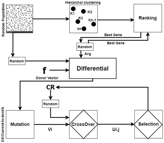
Figure 1. The framework of agglomerative-clustering-based differential evolution.

The proposed Equation (16) explains that the donor vector will be formed by calculating the differential between randomly selected clusters. In each iteration, the donor vector is generated by utilizing randomly selected different clusters.

The proposed scheme utilizes an adaptive crossover strategy. The crossover rate is adapted according to the fitness value of the newly created offspring. If the objective function value of the newly created offspring is better than that of the target vector, then CR_L (crossover large) value will be used in the selection phase and CR_S (crossover small) otherwise. The large and small values of the crossover rate ensure that the best is included in the population in each iteration. In the last stage of the proposed differential evolution scheme, either a newly created gene U_i,j is selected and added to the population, or X_i,j retains its position. Not only the newly created vector is included in the population, but it is inserted into the most relevant cluster, based on the prediction method of agglomerative clustering.

4.2. Proposed Algorithm

The proposed algorithm is a comprehensive enlistment of the entire process of this study.

Algorithm 1: Clustering-based self-adaptive DE

It starts with the creation of a random population within the given bounds of each benchmark function. Before beginning the next process, it is ensured that each gene/vector of this synthetic population is within the given bounds of the benchmark function. This population is fed to the clustering mechanism that generates the dendrogram for the entire population. This dendrogram helps in deciding the number of clusters “k” to be created by the hierarchal agglomerative clustering mechanism. Each cluster is separately stored and sorted in descending order (as we are solving the minimization problem). Once the clusters are formed, the best gene from randomly chosen clusters is fetched and passed to the mutation operation. The differential between the fetched genes is calculated as per the novel DE\k-Relative Best\1 policy. Upon completion of the mutation process, a donor vector U_i,j is produced. Next, the algorithm creates an offspring by the process of crossover between the trial vector U_i,j, and the target vector V_i.

The last phase of the entire process is to decide whether we will retain the existing target vector, or it will be replaced by a newly created trial vector. The best between the both remains in the population. If it happens to be the newly created trial vector, then the algorithm predicts the relevant cluster and inserts it into it. At each iteration, both the population clustering and adaptive CR value ensure that only the genes with improved performance are included in the population.

5. Benchmark Functions and Experimental Settings

To test the performance of the proposed algorithm, thirteen of the most complex benchmark functions from CEC2005 are used. The details of these functions are provided in Table 2. We have implemented these benchmarks in our experiments as a minimization problem. These functions are grouped into two categories: shifted unimodal and shifted multimodal. These benchmark functions were introduced by Yao et al. [27]. These most complex benchmark functions were introduced in a special session on real-parameter optimization of CEC 2005 by Suganthan et al. [28]. The parametric setting is exactly as in [23], i.e., NP is set to 1000, F is at 0.5, and the CR is initially at 0.7. Average values of error rate and standard deviation are obtained after running the algorithm for each benchmark function several times. Each time, 100 iterations are performed for each benchmark. For all benchmark functions, approximately after 100 iterations, the proposed policy reached optimal point.

Table 2. Test suit with 13 most complex benchmark functions presented in EC2005.

Type	f (x)	Name	Search Range	Global Optimum
Shifted Unimodal	f1	$f_1\left(x\right)={\displaystyle {\displaystyle \sum }_{i=1}^D}{z}_i^2+f_{bias}, z=x-o,x=[x_{1,}{x}_2\dots ,x_D]$	[−100, 100]	−450
	f2	$f_2\left(x\right)={\displaystyle {\displaystyle \sum }_{i=1}^D}{({\displaystyle {\displaystyle \sum }_{j=1}^i}{z}_j)}^2+f_{bias}, z=x-o,x=[x_{1,}{x}_2\dots ,x_D]$	[−100, 100]	−450
	f3	$f_3\left(x\right)={\displaystyle {\displaystyle \sum }_{i=1}^D}{\left({10}^6\right)}^{\frac{i-1}{D-1}}{z}_i^2+f_{bias}, z=\left(x-o\right)\ast M,,x=[x_{1,}{x}_2\dots ,x_D]$	[−100, 100]	−450
	f4	$f_4\left(x\right)=( {\displaystyle {\displaystyle \sum }_{i=1}^D}{({\displaystyle {\displaystyle \sum }_{j=1}^i}{z}_j)}^2)\ast \left(1+0.4\left|N\left(0,1\right)\right|\right)+f-bia{s}_4,z=x-o,x=[x_{1,}{x}_2\dots ,x_D]$	[−100, 100]	−450
	f5	$f\left(x\right)=\max \{\left|x_1+2x_2-7\right|,|2x_1+x_2-5\left|\right\},i=1,\dots ,n, X^{*}=\left[1,3\right],f\left(X^{*}\right)=0$	[−100, 100]	−310
Shifted Multimodal	f6	$f_6\left(x\right)={\displaystyle {\displaystyle \sum }_{i=1}^D}\left(100{(z_i^2-z_{i+1})}^2+{\left(z_1-1\right)}^2\right)+f_{bias}, z=x-o,x=[x_{1,}{x}_2\dots ,x_D]$	[−100, 100]	390
	f7	$f_8\left(x\right)=-20\exp (-0.2\sqrt{\frac{1}{D}{\displaystyle {\displaystyle \sum }_{i=1}^D}{z}_i^2)-\exp (\frac{1}{D}{\displaystyle {\displaystyle \sum }_{i=1}^D}\cos (2\pi z_i}))+20+e+f\_bias,z=\left(x-o\right)\ast M$	[−32, 32]	−140
	f8	$f_9\left(x\right)={\displaystyle {\displaystyle \sum }_{i=1}^D}(z_i^2-10\cos \left(2\pi z_i\right)+10)+f\_bias,z=x-o,x=x_1,x_{2,}\dots ,x_D$	[−5, 5]	−140
	f9	$f_{10}\left(x\right)={\displaystyle {\displaystyle \sum }_{i=1}^D}(z_i^2-10\cos \left(2\pi z_i\right)+10)+f\_bias,z=x-o\ast M,x=x_1,x_{2,}\dots ,x_D$	[−5, 5]	−330
	f10	$f_{11}\left(x\right)={\displaystyle {\displaystyle \sum }_{i=1}^D}({\displaystyle {\displaystyle \sum }_{k=0}^{kmax}}\left[a^k\cos \left(2\pi b^k\left(z_i+0.5\right)\right)\right])-D{\displaystyle {\displaystyle \sum }_{k=0}^{kmax}}[a^k\cos \left(2\pi b^k\left(z_i\mathrm{.0.5}\right)\right]+f_{bias}$	[−0.5, 0.5]	90
	f11	$f_{12}\left(x\right)={\displaystyle {\displaystyle \sum }_{i=1}^D}{\left(A_i-B_i\left(x\right)\right)}^2+f\_bias$	[−3.14, 3.14]	−460
	f12	$f_8\left(x\right)={\displaystyle {\displaystyle \sum }_{i=1}^D}\frac{x_i{}^2}{4000}-{\displaystyle {\displaystyle \prod }_{i=1}^D}\cos \left(\frac{x_i}{\sqrt{i}}\right)+1$	[−3, 1]	−130
	f13	$f\left(x,y\right)=0.5+\frac{{\sin }^2(\sqrt{x^2+y^2)-0.5}}{1+0.001{\left(x^2+y^2\right)}^2}$	[−100, 100]	−300

The experiments were run on Google’s GPU having Intel (R) Xeon (R) with a 2.30 GHz dual-core processor of Haswell Family having 12 GB of RAM and 25 GB storage space.

6. Performance Evaluation Parameters

The performance of the proposed strategy is tested in terms of error rate and, improvement number, and the number of times CR_L and CR_s are used

The error rate, calculated by Equation (17), is the difference between the trial vector and the target vector in terms of the objective function value.

$$ErroRate={{\displaystyle \sum }}_{i=1}^{iter}f\left(x_{trial}\right)-f\left(x_{target}\right)$$

(17)

where iter is the presets of the number of iterations, and f (x) is the objective function value for trial and target vectors. The improvement number is calculated by measuring the difference between the trial vector’s value and the value of the pre-existing vector.

7. Results and Discussion

This section explains the results attained by ABCDE against the classical variants, e.g., random and best mutation policies, and against the state-of-the-art policy, e.g., random neighborhood DE. Table 3 displays the average error rates and their corresponding standard deviations for each of the benchmark functions. The proposed algorithm was run multiple times for each function to obtain these values. The best result for each benchmark is highlighted in bold, while the runner-up values are underlined. It is noteworthy that the ABCDE algorithm outperformed its counterparts by a significant margin for all thirteen of the most complex functions in CEC 2005. This can be attributed to the clustering mechanism and self-adaptiveness employed in the algorithm. In Table 3, a comparison is presented among DE/rand/1, DE/best/1, RNDE, and ABCDE. All values for ABCDE are negative, indicating that, on average, the algorithm never generated a gene with a lower objective value than that of the target vector. It consistently produced objective values that were equal to or better than those of its counterparts.

Table 3. Experimental results showing average error ± standard deviation of random, best, random neighborhood and proposed mutation policies at D = 30 and iterations = 100.

f(x)	DE/Rand/1	DE/Best/1	RNDE	ABCDE
f1	0.00 × 10−00 ± 0.00 × 10−00	3.64 × 10−13 ± 2.62 × 10−13	0.00 × 10+00 ± 0.00 × 10+00	−6.59 × 10+03 ± 9.25 × 10+03
f2	4.15 × 10−05 ± 3.95 × 10−05	1.18 × 10−12 ± 7.06 × 10−13	1.53 × 10−13 ± 8.19 × 10−14	−2.34 × 10+05 ± 4.13 × 10+05
f3	3.54 × 10+05 ± 1.86 × 10+05	1.39 × 10+04 ± 1.08 × 10+04	1.63 × 10+05 ± 1.00 × 10+05	−1.29 × 10+13 ± 4.10 × 10+13
f4	1.82 × 10−02 ± 2.54 × 10−02	2.06 × 10+02 ± 3.50 × 10+02	4.10 × 10−04 ± 6.38 × 10−04	−1.28 × 10+06 ± 2.24 × 10+06
f5	5.78 × 10+01 ± 6.45 × 10+01	2.09 × 10+03 ± 7.14 × 10+02	1.22 × 10+02 ± 1.95 × 10+02	−2.74 × 10+03 ± 4.50 × 10+03
f6	1.90 × 10−01 ± 8.27 × 10−01	1.06 × 10+00 ± 1.76 × 10+00	1.33 × 10−01 ± 7.16 × 10−01	−1.22 × 10+10 ± 2.46 × 10+10
f7	2.09 × 10+01 ± 4.67 × 10−02	2.09 × 10+01 ± 5.92 × 10−02	2.09 × 10+01 ± 5.10 × 10−02	−1.76 × 10+04 ± 1.79 × 10+05
f8	1.34 × 10+02 ± 2.23 × 10+01	1.06 × 10+02 ± 2.84 × 10+01	1.89 × 10−15 ± 1.02 × 10−14	−1.99 × 10+01 ± 2.43 × 10+01
f9	1.83 × 10+02 ± 8.39 × 10+00	1.53 × 10+02 ± 3.95 × 10+01	1.12 × 10+02 ± 1.20 × 10+01	−4.99 × 10+01 ± 3.40 × 10+03
f10	3.97 × 10+01 ± 1.13 × 10+00	2.12 × 10+01 ± 3.14 × 10+00	3.24 × 10+01 ± 1.02 × 10+00	−1.81 × 10+00 ± 2.21 × 10+00
f11	1.42 × 10+03 ± 2.98 × 10+03	1.27 × 10+03 ± 1.32 × 10+03	4.21 × 10+03 ± 1.12 × 10+04	−2.34 × 10+05 ± 3.79 × 10+05
f12	1.53 × 10+01 ± 9.23 × 10−01	6.53 × 10+00 ± 2.24 × 10+00	4.11 × 10+00 ± 2.98 × 10−01	−7.11 × 10+02 ± 1.63 × 10+03
f13	1.33 × 10+01 ± 1.21 × 10−18	1.19 × 10+01 ± 5.42 × 10−01	1.30 × 10+01 ± 1.55 × 10−01	−4.48 × 10+15 ± 8.47 × 10+15

The reason behind this achievement is the utilization of the best gene for the production of the donor vector. This approach clusters the population to group similar genes and then sorts each cluster in descending order to place the best value at the top. To create a donor vector, the proposed ABCDE algorithm selects the top value from a randomly chosen cluster. For the shifted sphere function, both RNDE and DE/rand/1 policies produced genes with objective function values that were the same as those of the trial and target vectors. In contrast, the ABCDE algorithm produced genes with objective function values that were better than the target vector’s objective function value, with an average of 6.59E03 and a standard deviation of 9.25E+03.

For the Shifted Schwefel benchmark function, RNDE produced genes that were better than the target vector, with an average error of 1.53E−13 and a standard deviation of 8.19E−14. However, the ABCDE algorithm outperformed RNDE with an average of −2.34E+05 and a standard deviation of 4.13E+05. In the case of the Shifted Rotated High Conditioned Elliptical Function benchmark, DE/Best/1 produced results with an average error of 1.39E+04 and a standard deviation of 1.08E+04. However, the ABCDE algorithm produced better objective values, with an average of −1.29E+13 and a standard deviation of ±4.10E+13. In the Shifted Schwefel Problem 1.3 with Noise in Fitness benchmark, RNDE came in second place and had an average error rate of 4.10E−04 with a standard deviation of 6.38E−04. In comparison, ABCDE performed better in the f4 benchmark with an average improvement of −1.28E+06 and reached the Global Optimum on Bounds, which was the last of the unimodal benchmarks. For the rest of the multimodal benchmarks, ABCDE consistently produced superior genes that achieved lower objective values of trial vectors.

For the Shifted Rosenbrocks and Shifted Rotated Ackley with Global Optimum on Bounds benchmarks, the error rate and standard deviation were 1.33E−01 ± 7.16E−01 and 2.09E+01 ± 4.67E−02, respectively. ABCDE produced genes without any inferior objective values for both of these functions. The average success rate for ABCDE, with standard deviation, was 1.22E+10±2.46E+10 and −1.76E+04±1.79E+05. For Shifted Rastrigin, Shifted Rotated Rastrigin, Shifted Rotated Weierstrass, Schwefel Problem 2.13, and Shifted Expanded Griewank plus Rosenbrock (F8F2), ABCDE outperformed DE/Best/1, DE/Best/1, and RNDE, respectively. The scores of ABCDE for these five benchmarks were −1.99E+01, −4.99E+01, −1.81E+00, −2.34E+05, and −7.11E, respectively, and the standard deviations are shown in Table 3.

Of all the 13 benchmarks, ABCDE performed best in the Shifted Rotated Expanded Scaffer’s F6 benchmark function, significantly outperforming its counterparts. Compared to its nearest competitor, DE/Best/1, ABCDE achieved an average of 4.48E+15, with a standard deviation of 8.47E+15. Figure 2a,b show the yielded improvement in each iteration for different unimodal and multimodal benchmarks, respectively. The common thing among all is a gradual and rapid decrease between the generated trial vector and the existing target vector. The behavior of ABCDE remained consistent throughout the 100 iterations, and achieved optimal convergence for all benchmark functions.

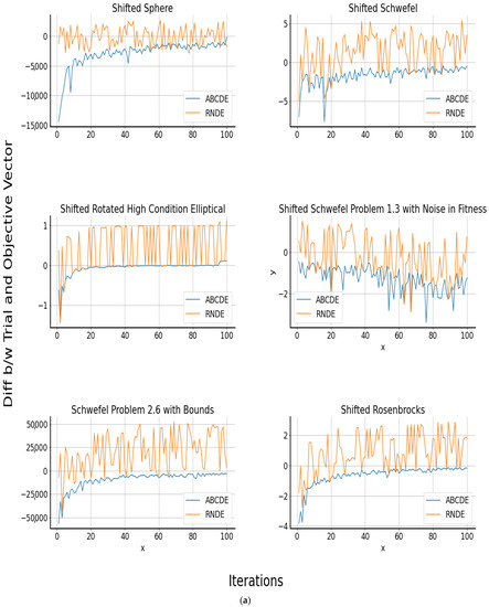
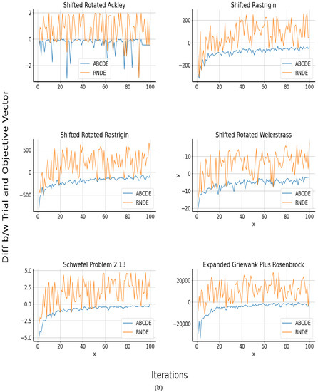
Figure 2. (a) Improvement rate of shifted unimodal benchmark functions at D = 30 and iter = 100. (b) Improvement rate of shifted multimodal benchmark functions at D = 30 and iter = 100.

By the 100th iteration, ABCDE had the smallest difference between the trial vector and the objective vector. On the other hand, RNDE fluctuated considerably and was still exploring the population by the 100th iteration. For all benchmark functions, the improvement observed in RNDE was minimal. For the Shifted Sphere function, it can be seen that at the start of the process, the difference between the trial vector and the target vector’s values was the greatest. It was almost about 150,000 units. However, with more and more iteration, the difference kept decreasing. The value of the difference reduced to 55,000 for the sixth iteration, but for the seventh iteration, it again jumped to 97,000. This pattern shows that the population had the local optima in it, which was managed well by the ABCDE as it utilized a random selection of clusters for generating donor vectors. For the Shifted Schwefel function, the graph shows that the local optima were induced at about the seventeenth iteration. This was followed by a few smaller local optimal positions in the population, but ABCDE can adapt to the situation accordingly. The graph for Shifted Rotated High Condition Elliptical function shows that the population for this benchmark converged very rapidly without any major local optima. However, for Shifted Schwefel 1.3 with Noise in Fitness function, it is eminent that 100 iterations were not enough for it to converge properly.

It started with little difference between the calculated and actual values, but with time, the difference became wider by the end of 100 iterations. Certainly, this function required more iterations to converge to any stable point. The pattern of convergence was identical for most of the unimodal and multimodal benchmarks. For Shifted Rotated Ackley function, the pattern was very polarized. In a few iterations, the difference between the offspring vector and the existing vector was at the very minimum, but suddenly in the next iteration, it reached a new high point. This validates the opinion that the generated population was very complex and had many local optima in it. For all of the unimodal and multimodal functions, the initial population is clustered into K number of clusters before applying the mutation procedure.

The clustering of population groups together the most similar genes in the entire population, and hence the chance of becoming trapped in local optima are reduced. Furthermore, at each iteration, if the trial vector is to replace the target vector, it is inserted into a proper cluster predicted by the agglomerative clustering mechanism. This is the reason why the population converged quite rapidly for each of the benchmark functions. The self-adaptive feature ensured the inclusion of only better genes into the population at each iteration. At each insertion, the population is refreshed for the number of candidate genes in the population, and also the clusters are re-ranked. Once a new gene is inserted into the relevant cluster, it is sorted again.

Figure 3 presents the summary of all four contestants for thirteen most complex benchmarks. It indicates that ABCDE always has the lowest curve pattern for all benchmarks shown on the x-axis. The y-axis gives the average error rate achieved, which is written in scientific notations. Other than the proposed strategy, all three policies yielded results that were quite similar to each other. However, the graph shoes that ABCDE outperforms all others by a fair margin due to its double-step (clustering and intelligent adaptiveness) policy.

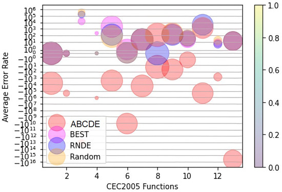
Figure 3. Error rate comparison of ABCDE for all benchmark functions.

Figure 4 shows a relationship between two adaptions of crossover rate CR. This study utilized an adaptive crossover rate policy. Whenever the proposed DE/Current-to-best/K mutation policy produced a gene that had a better objective value than the existing vector, ABCDE utilized a higher level of crossover rate and adopted approximately 85% from the donor vector. At the same time, when our proposed mutation policy could not generate a gene with a better objective value, we took as low as less than 1% from the donor vector. It can be seen that an average for the shifted sphere benchmark function, 20% of the time, DE/Current-to-best/K yielded better results. For the remaining 80% of the time, we adopted almost nothing from the donor vector and ensured that no lesser than the current gene was inserted into the population.

Figure 4. Crossover large/small usage in percentage.

For Shifted Schwefel Problem 1.2, Shifted Rotated Ackley with Global Optimum on Bounds, and Shifted Rotated Weierstrass benchmarks, our proposed mutation policy produced the least percentage of better genes. For all these situations, the self-adaptive crossover rate complimented the poor performance and obstructed the inclusion of sick genes. For Shifted Rosenbrocks benchmark function, our proposed mutation strategy produced the highest 23% of genes that were better than the existing ones. For all of the 13 benchmark functions, due to the clustering and intelligent adaption of CR, ABCDE comprehensively outperformed its counterparts by some margin. It can be seen that for ABCDE, all the obtained values are in the negative plane, which indicates that for no instance ABCDE generated offspring erroneously. Whenever ABCDE could not produce a favorable offspring, its weakness was complimented by intelligent adaption of CR value. Because of this double-check policy, in each iteration, no bad vector was inserted into the population, and hence the population converged very rapidly.

Lastly, Table 4 displays the data on the scalability of the proposed approach, compared to RNDE, with respect to accuracy, change in accuracy, clock time elapsed for simulation, and time-to-population ratio for each gene.

Table 4. Scalability statistics of ABCDE against RNDE.

Population	Max Error		Change in Error		Clock Time (s)		Time/Population Ratio
	ABCDE	RNDE	ABCDE	RNDE	ABCDE	RNDE	ABCDE	RNDE
10	0.0080	0.0080	0.0000	0.0000	11	11	1.10	1.10
100	0.3450	0.5034	0.3370	0.4954	105	105	1.05	1.05
1000	0.6359	1.5963	0.2909	0.0929	1260	1620	1.26	1.62
10000	0.9029	2.2908	0.2670	0.6945	15900	21400	1.59	2.14

Superior values are highlighted in bold. Initially, both contenders performed equally well when the population was set to 10, but as the population size increased, the accuracy of RNDE suffered significantly. In contrast, the change in accuracy of ABCDE remained consistent for all population variations. Additionally, the clock time required for running the simulation was notably different for both approaches. For the maximum input population, ABCDE took 15,900 s to converge, while RNDE took 21,400 s. This achievement is attributed to a balanced mutation strategy, combined with an adaptive crossover rate. ABCDE re-inserted only positive genes at each iteration, enabling it to converge rapidly without becoming trapped in local optima.

8. Conclusions and Future Work

Differential evolution is a very powerful evolutionary algorithm that has proved its worth in many of the CEC competitions for numerical optimization. The key to the success of differential evolution is its balanced mutation strategy. The mutation policies are categorized into two main branches: exploration-based and exploitation-based. Both of these are opposites to each other. One achieves high accuracy while the other converges very quickly. To achieve both, we need to strike a perfect balance between the two. To achieve this, a novel agglomerative-clustering-based self-adaptive differential evolution policy is proposed in this study. The proposed ABCDE strategy is tested for 13 of the most complex unimodal and multimodal benchmark functions presented in CEC 2005.

In comparison with classical and contemporary differential evolution schemes (RNDE), we have proved that ABCDE is a far better scheme, and for the 13 most complex functions of CEC 2005, the error rate is as low as <1% for some of the benchmark functions. The fast convergence of differential evolution makes it a valuable tool in various fields where optimization problems need to be solved quickly and accurately. The fast convergence of differential evolution can be a useful tool in cloud computing for optimizing resource allocation, SLAs, energy efficiency, load balancing, and resource scheduling. The fast convergence of differential evolution can also have several applications in symmetry, including crystallography, symmetry detection, image analysis, pattern recognition, and optimization of optical systems.

Agglomerative clustering can suffer from the “chaining” effect, where the algorithm tends to create long chains of small clusters instead of forming larger, more cohesive clusters. In the future, we will modify the standard agglomerative clustering mechanism to complement this drawback and to avoid any suboptimal results. We also plan to test differential evolution’s performance on the most recent benchmark function such as CEC 2020. For application, this exceedingly well-performing differential evolution approach can be utilized for optimizing the weights of an artificial neural network. This will enable us to train an ANN quickly, and hence open a gateway for the ANNs to be used in time-constrained environments such as cloud computing.

References

- Yan, X.; Tian, M. Differential Evolution with Two-Level Adaptive Mechanism for Numerical Optimization. Knowl.-Based Syst. 2022, 241, 108209. [Google Scholar] [CrossRef]
- Ahmad, M.F.; Isa, N.A.M.; Lim, W.H.; Ang, K.M. Differential Evolution: A Recent Review Based on State-of-the-Art Works. Alex. Eng. J. 2022, 61, 3831–3872. [Google Scholar] [CrossRef]
- Strnad, I.; Marsetič, R. Differential Evolution Based Numerical Variable Speed Limit Control Method with a Non-Equilibrium Traffic Model. Mathematics 2023, 11, 265. [Google Scholar] [CrossRef]
- Al-Dabbagh, R.D.; Neri, F.; Idris, N.; Baba, M.S. Algorithmic Design Issues in Adaptive Differential Evolution Schemes: Review and Taxonomy. Swarm Evol. Comput. 2018, 43, 284–311. [Google Scholar] [CrossRef]
- Pant, M.; Zaheer, H.; Garcia-Hernandez, L.; Abraham, A. Differential Evolution: A Review of More than Two Decades of Research. Eng. Appl. Artif. Intell. 2020, 90, 103479. [Google Scholar] [CrossRef]
- Price, K.V.; Storn, R.M.; Lampinen, J.A. Differential Evolution. A Practical Approach to Global Optimization; Springer Science & Business Media: Berlin, Germany, 2005. [Google Scholar]
- Deng, L.; Sun, H.; Zhang, L.; Qiao, L. N-CODE: A Differential Evolution with n-Cauchy Operator for Global Numerical Optimization. IEEE Access 2019, 7, 88517–88533. [Google Scholar] [CrossRef]
- Zhou, X.G.; Zhang, G.J. Differential Evolution with Underestimation-Based Multimutation Strategy. IEEE Trans. Cybern. 2019, 49, 1353–1364. [Google Scholar] [CrossRef]
- Ge, Y.F.; Yu, W.J.; Lin, Y.; Gong, Y.J.; Zhan, Z.H.; Chen, W.N.; Zhang, J. Distributed Differential Evolution Based on Adaptive Mergence and Split for Large-Scale Optimization. IEEE Trans. Cybern. 2018, 48, 2166–2180. [Google Scholar] [CrossRef]
- Jadon, S.S.; Tiwari, R.; Sharma, H.; Bansal, J.C. Hybrid Artificial Bee Colony Algorithm with Differential Evolution. Appl. Soft Comput. J. 2017, 58, 11–24. [Google Scholar] [CrossRef]
- Zhan, C.; Situ, W.; Yeung, L.F.; Tsang, P.W.M.; Yang, G. A Parameter Estimationmethod for Biological Systems Modelled by ODE/DDE Models Using Splineapproximation and Differential Evolution Algorithm. IEEE/ACM Trans. Comput. Biol. Bioinform. 2014, 11, 1066. [Google Scholar] [CrossRef] [PubMed]
- Zhao, J.; Xu, Y.; Luo, F.; Dong, Z.; Peng, Y. Power System Fault Diagnosis Based on History Driven Differential Evolution and Stochastic Time Domain Simulation. Inf. Sci. 2014, 275, 13–29. [Google Scholar] [CrossRef]
- Paul, S.; Das, S. Simultaneous Feature Selection and Weighting—An Evolutionary Multi-Objective Optimization Approach. Pattern Recognit. Lett. 2015, 65, 51–59. [Google Scholar] [CrossRef]
- Peng, H.; Guo, Z.; Deng, C.; Wu, Z. Enhancing Differential Evolution with Random Neighbors Based Strategy. J. Comput. Sci. 2018, 26, 501–511. [Google Scholar] [CrossRef]
- Chiang, C.W.; Lee, W.P.; Heh, J.S. A 2-Opt Based Differential Evolution for Global Optimization. Appl. Soft Comput. J. 2010, 10, 1200–1207. [Google Scholar] [CrossRef]
- Croes, G.A. A Method for Solving Traveling-Salesman Problems. Oper. Res. 1958, 6, 791–812. [Google Scholar] [CrossRef]
- Epitropakis, M.G.; Tasoulis, D.K.; Pavlidis, N.G.; Plagianakos, V.P.; Vrahatis, M.N. Enhancing Differential Evolution Utilizing Proximity-Based Mutation Operators. IEEE Trans. Evol. Comput. 2011, 15, 99–119. [Google Scholar] [CrossRef]
- Ali, M.M. Differential Evolution with Generalized Differentials. J. Comput. Appl. Math. 2011, 235, 2205–2216. [Google Scholar] [CrossRef]
- Zhou, Y.; Li, X.; Gao, L. A Differential Evolution Algorithm with Intersect Mutation Operator. Appl. Soft Comput. J. 2013, 13, 390–401. [Google Scholar] [CrossRef]
- Meng, Z.; Pan, J.S.; Tseng, K.K. PaDE: An Enhanced Differential Evolution Algorithm with Novel Control Parameter Adaptation Schemes for Numerical Optimization. Knowl.-Based Syst. 2019, 168, 80–99. [Google Scholar] [CrossRef]
- Wu, G.; Shen, X.; Li, H.; Chen, H.; Lin, A.; Suganthan, P.N. Ensemble of Differential Evolution Variants. Inf. Sci. 2018, 423, 172–186. [Google Scholar] [CrossRef]
- Liu, Q.; Du, S.; van Wyk, B.J.; Sun, Y. Double-Layer-Clustering Differential Evolution Multimodal Optimization by Speciation and Self-Adaptive Strategies. Inf. Sci. 2021, 545, 465–486. [Google Scholar] [CrossRef]
- Cai, Y.; Wu, D.; Zhou, Y.; Fu, S.; Tian, H.; Du, Y. Self-Organizing Neighborhood-Based Differential Evolution for Global Optimization. Swarm Evol. Comput. 2020, 56, 100699. [Google Scholar] [CrossRef]
- Mansour, R.F.; Alhumyani, H.; Khalek, S.A.; Saeed, R.A.; Gupta, D. Design of Cultural Emperor Penguin Optimizer for Energy-Efficient Resource Scheduling in Green Cloud Computing Environment. Clust. Comput. 2023, 26, 575–586. [Google Scholar] [CrossRef]
- Rana, N.; Abd Latiff, M.S.; Abdulhamid, S.M.; Misra, S. A Hybrid Whale Optimization Algorithm with Differential Evolution Optimization for Multi-Objective Virtual Machine Scheduling in Cloud Computing. Eng. Optim. 2022, 54, 1999–2016. [Google Scholar] [CrossRef]
- Xue, Y.; Tong, Y.; Neri, F. An Ensemble of Differential Evolution and Adam for Training Feed-Forward Neural Networks. Inf. Sci. 2022, 608, 453–471. [Google Scholar] [CrossRef]
- Yao, X.; Liu, Y.; Lin, G. Evolutionary Programming Made Faster. IEEE Trans. Evol. Comput. 1999, 3, 82–102. [Google Scholar] [CrossRef]
- Suganthan, P.N.; Hansen, N.; Liang, J.J.; Deb, K.; Chen, Y.P.; Auger, A.; Tiwari, S. Problem Definitions and Evaluation Criteria for the CEC 2005 Special Session on Real-Parameter Optimization. Technical Report, Nanyang Technological University, Singapore and KanGAL Report Number 2005005 (Kanpur Genetic Algorithms Laboratory, IIT Kanpur). May 2005. Available online: http://www.cmap.polytechnique.fr/~nikolaus.hansen/Tech-Report-May-30-05.pdf (accessed on 1 March 2023).
Disclaimer/Publisher’s Note: The statements, opinions and data contained in all publications are solely those of the individual author(s) and contributor(s) and not of MDPI and/or the editor(s). MDPI and/or the editor(s) disclaim responsibility for any injury to people or property resulting from any ideas, methods, instructions or products referred to in the content. |
© 2023 by the authors. Licensee MDPI, Basel, Switzerland. This article is an open access article distributed under the terms and conditions of the Creative Commons Attribution (CC BY) license (https://creativecommons.org/licenses/by/4.0/).