Fractional Differential Equations and Expansions in Fractional Powers

Abstract

We use power series with rational exponents to find exact solutions to initial value problems for fractional differential equations. Certain problems that have been previously studied in the literature can be solved in a closed form, and approximate solutions are derived by constructing recursions for the relevant expansion coefficients.

1. Introduction

The field of fractional integrals and derivatives is vast, and its importance is increasing daily due to its numerous applications. Different definitions have been proposed, leading to several approaches to the subject. It is worth noting that all existing types of fractional integro-differentiation operators are discussed in the book by S. Samko, A. A. Kilbas, and O. Marichev [1], along with the applications of fractional calculus to different equations, including the first-order integral equation, the Euler–Poisson–Darboux-type equations, and differential equations of fractional order. It is worth examining the findings presented in [2,3], where several extensions are proposed.

In this research study, we only use the Euler and Caputo definitions for fractional derivatives, without delving into the complex framework surrounding it. Our goal is to demonstrate that we can find solutions to certain types of initial value problems for fractional differential equations by making judicious use of power series expansions with rational exponents. It is worth noting that the powers used in these expansions exhibit a natural symmetry, as they are integer multiples of a given number $\alpha$, where $0<\alpha <1$.

It should be noted that the method being discussed in this context, which is essentially the indeterminate coefficient method, may not be suitable for solving every problem of this nature. However, this technique is worth exploring in greater depth, as it can often be adapted to the equation being studied, thereby avoiding the need for the more complex techniques outlined in the cited bibliography [4,5,6,7,8,9,10,11,12].

It is worth noting that the same approach can be applied to the solution of more general equations as well as to the evaluation of the approximation errors, as shown by G. Groza and M. Jianu [13]. Please note that in our case we are finding exact solutions, and as such the aforesaid step is unnecessary.

In the final section of this paper, we utilize the same methodology to obtain an approximate solution to the fractional-order logistic equation. A similar approach can be found in the articles of M. Ortigueira et al. [14,15,16], which were recently shared with us by the author after our article in MDPI Symmetry [17] was published. We encourage interested readers to refer to these articles for further information.

2. Fractional Derivative of Powers

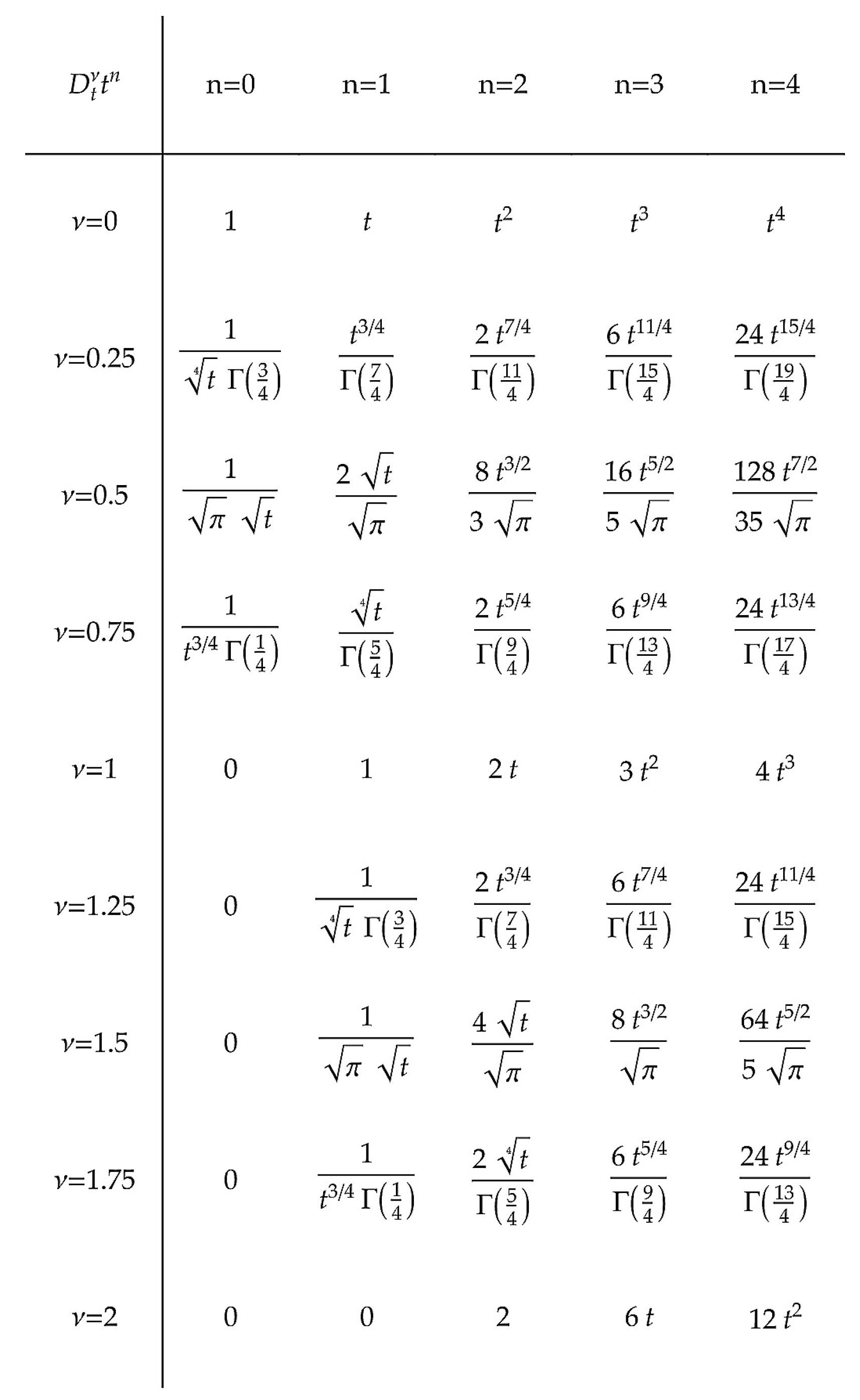
The definition of the fractional derivative of a power function dates back to Euler, and falls within the definition of fractional derivatives introduced by Caputo as a special case:

$$\begin{array}{c}\left\{\begin{array}{c}{\displaystyle D_t^{\nu }{t}^n=\frac{\mathrm{\Gamma }(n+1)}{\mathrm{\Gamma }(n+1-\nu )}{t}^{n-\nu },(n\ge \left[\nu \right]),}\\ D_t^{\nu }{t}^n=0,(n<\left[\nu \right]),\end{array}\right.\end{array}$$

(1)

where n and $\nu$ are rational numbers and $\left[\nu \right]$ denotes the integral part of $\nu$. If c is a constant, then $D_t^{\nu }c=0$.

As is known from theory, the Caputo derivative is defined in the following way [18]:

$$\begin{array}{c}\hfill {\displaystyle D_{a+}^{\nu }f\left(t\right)=\frac{1}{\mathrm{\Gamma }(n-\nu )}{\int }_a^t\frac{f^{\left(n\right)}\left(\tau \right)}{{(t-\tau )}^{\nu -n+1}}d\tau ,(n\ge \left[\nu \right]),}\end{array}$$

and reduces to (1) when $a=0$ and $f\left(t\right)=t^n$.

Particular Cases

As an example, when $\nu =1/2$ and n is an integer, we find that

$$\begin{array}{c}\hfill {\displaystyle D_t^{1/2}{t}^n=\frac{n!}{\mathrm{\Gamma }(n+\frac{1}{2})}{t}^{n-\frac{1}{2}},(n\ge 1),}\end{array}$$

(2)

and more generally, for $\nu =(2k+1)/2$ with $(k=1,2,\dots )$,

$$\begin{array}{c}\hfill \begin{array}{c}{\displaystyle D_t^{3/2}{t}^n=\frac{n!}{\mathrm{\Gamma }(n-1/2)}{t}^{n-3/2},D_t^{5/2}{t}^n=\frac{n!}{\mathrm{\Gamma }(n-3/2)}{t}^{n-5/2},}\\ {\displaystyle \phantom{1pt26pt}{D}_t^{N-1/2}{t}^n=\frac{n!}{\mathrm{\Gamma }(n-N+3/2)}{t}^{n-N+1/2},}\end{array}\end{array}$$

where

$$\begin{array}{c}\hfill {\displaystyle \mathrm{\Gamma }(1/2)=\sqrt{\pi },\mathrm{\Gamma }(3/2)=\frac{\sqrt{\pi }}{2},\dots ,\mathrm{\Gamma }(n+1/2)=\frac{(2n-1)!!}{2^n}\sqrt{\pi }.}\end{array}$$

The first few examples of fractional derivatives of powers are shown in the Appendix A at the end of this article.

3. Expansion in Fractional Powers

We define the expansion of an analytic function $f\left(t\right)$ in terms of fractional powers as per the following expression:

$$\begin{array}{c}\hfill \begin{array}{c}{\displaystyle f\left(t\right)=a_0+\frac{a_1}{\mathrm{\Gamma }(3/2)}{t}^{1/2}+\frac{a_2}{\mathrm{\Gamma }(5/2)}{t}^{3/2}+\frac{a_3}{\mathrm{\Gamma }(7/2)}{t}^{5/2}+\cdots +\frac{a_n}{\mathrm{\Gamma }(n+1/2)}{t}^{n-1/2}+\dots =}\\ {\displaystyle \phantom{1pt26pt}{a}_0+\sum _{n=1}^{\infty }\frac{a_n}{\mathrm{\Gamma }(n+1/2)}{t}^{n-1/2}.}\end{array}\end{array}$$

(3)

This is a formal expansion, and series convergence aspects are not considered here, as only a finite number of terms is considered in the following.

The meaning of the expansion coefficients is as follows.

Of course, we have $a_0=f\left(0\right)$; as it is possible to exchange the Caputo fractional derivative $D^{1/2}$ with the series symbol (see [18]), we find

$$\begin{array}{c}\hfill {\displaystyle D_t^{1/2}{f\left(t\right)|}_{(t=0)}=\frac{a_1}{\mathrm{\Gamma }(3/2)}{D}_t^{1/2}{t}^{1/2}{{|}_{(t=0)}+\frac{a_2}{\mathrm{\Gamma }(5/2)}{D}_t^{1/2}{t}^{3/2}|}_{(t=0)}+\dots ,}\end{array}$$

that is,

$$\begin{array}{c}\hfill {\displaystyle D_t^{1/2}f\left(t\right){|}_{(t=0)}=\frac{a_1}{\mathrm{\Gamma }(3/2)}\frac{\mathrm{\Gamma }(3/2)}{\mathrm{\Gamma }\left(1\right)}+\frac{a_2}{\mathrm{\Gamma }(5/2)}\frac{\mathrm{\Gamma }(5/2)}{\mathrm{\Gamma }\left(2\right)}t{|}_{(t=0)}+0+\cdots =a_1,}\end{array}$$

$$\begin{array}{c}\hfill \begin{array}{c}{D}_t^{3/2}\left({\displaystyle f\left(t\right)-a_0-\frac{a_1}{\mathrm{\Gamma }(3/2)}{t}^{1/2}}\right){|}_{(t=0)}=\\ \phantom{1pt26pt}{D}_t^{3/2}\left({\displaystyle \frac{a_2}{\mathrm{\Gamma }(5/2)}{t}^{3/2}+\frac{a_3}{\mathrm{\Gamma }(7/2)}{t}^{5/2}+\cdots +\frac{a_n}{\mathrm{\Gamma }(n+1/2)}{t}^{n-1/2}+\dots }\right){|}_{(t=0)}=\\ \phantom{1pt30pt}\left({\displaystyle \frac{a_2}{\mathrm{\Gamma }(5/2)}\frac{\mathrm{\Gamma }(5/2)}{\mathrm{\Gamma }\left(1\right)}+\frac{a_3}{\mathrm{\Gamma }(7/2)}\frac{\mathrm{\Gamma }(7/2)}{\mathrm{\Gamma }\left(2\right)}t+\frac{a_3}{\mathrm{\Gamma }(7/2)}\frac{\mathrm{\Gamma }(7/2)}{\mathrm{\Gamma }\left(3\right)}{t}^2+\dots }\right){|}_{(t=0)}=a_2,\end{array}\end{array}$$

and, for the general N-th coefficient,

$$\begin{array}{c}\hfill D_t^{(N-1/2)}\left({\displaystyle f\left(t\right)-a_0-\sum _{n=1}^{N-1}\frac{a_n}{\mathrm{\Gamma }(n+1/2)}{t}^{n-1/2}}\right){|}_{(t=0)}=a_N.\end{array}$$

Remark 1. 

Similar expansions could be obtained assuming $\nu =1/3,1/4,\dots$

Subsequent Derivatives of Order $1/2$

Considering the expansion in (3), we find

$$\begin{array}{c}\hfill \begin{array}{c}{\displaystyle D_t^{1/2}f\left(t\right)=a_1+a_{2}t+\frac{a_3}{2!}{t}^2+\frac{a_4}{3!}{t}^3+\cdots +\frac{a_{n+1}}{n!}{t}^n+\dots ,}\end{array}\end{array}$$

(4)

$$\begin{array}{c}\hfill \begin{array}{c}{\displaystyle D_{t}f\left(t\right)=D_t^{1/2}{D}_t^{1/2}f\left(t\right)=\frac{a_2}{\mathrm{\Gamma }(3/2)}{t}^{1/2}+\frac{a_3}{\mathrm{\Gamma }(5/2)}{t}^{3/2}+\frac{a_4}{\mathrm{\Gamma }(7/2)}{t}^{5/2}+\dots }\\ {\displaystyle \phantom{1pt26pt}+\frac{a_{n+1}}{\mathrm{\Gamma }(n+1/2)}{t}^{n-1/2}+\dots ,}\end{array}\end{array}$$

(5)

$$\begin{array}{c}\hfill {\displaystyle D_t{D}_t^{1/2}f\left(t\right)=D_t^{3/2}f\left(t\right)=a_2+a_{3}t+\frac{a_4}{2!}{t}^2+\cdots +\frac{a_{n+2}}{n!}{t}^n+\dots ,}\end{array}$$

(6)

$$\begin{array}{c}\hfill \begin{array}{c}{\displaystyle D_t^{2}f\left(t\right)=D_t^{1/2}{D}_t^{3/2}f\left(t\right)=\frac{a_3}{\mathrm{\Gamma }(3/2)}{t}^{1/2}+\frac{a_4}{\mathrm{\Gamma }(5/2)}{t}^{3/2}+\frac{a_5}{\mathrm{\Gamma }(7/2)}{t}^{5/2}+\dots }\\ {\displaystyle \phantom{1pt26pt}+\frac{a_{n+2}}{\mathrm{\Gamma }(n+1/2)}{t}^{n+1/2}+\dots .}\end{array}\end{array}$$

(7)

Other half-integer-order derivatives can be easily derived by noting that at each step it is sufficient to increase the index of the coefficients $a_n$ by one unit and leave the powers of the variable t unchanged.

In the following, we apply the method of indeterminate coefficients to solve initial value problems of fractional differential equations.

4. Examples

4.1. Example 1

Let us first consider the problem of finding a particular solution for the following inhomogeneous fractional equation [10]:

$$\begin{array}{c}\hfill \left\{\begin{array}{c}{\displaystyle D_t^{1/2}Z\left(t\right)+Z\left(t\right)=t^2+\frac{2}{\mathrm{\Gamma }(5/2)}{t}^{3/2},}\hfill \\ Z\left(0\right)=0.\hfill \end{array}\right.\end{array}$$

(8)

Set

$$\begin{array}{c}\hfill {\displaystyle Z\left(t\right)=\sum _{n=0}^{\infty }{a}_n\frac{t^n}{n!},}\end{array}$$

(9)

then, ${\displaystyle D_t^{1/2}(t^n/n!)=\frac{1}{\mathrm{\Gamma }(n+\frac{1}{2})}{t}^{n-\frac{1}{2}}}$.

Recalling that the Caputo differentiation under the series symbol holds for analytic functions, and considering that the fractional derivative of the first constant term vanishes, we can conclude that

$$\begin{array}{c}\hfill {\displaystyle \sum _{n=1}^{\infty }{a}_n\frac{1}{\mathrm{\Gamma }(n+\frac{1}{2})}{t}^{n-\frac{1}{2}}+\sum _{n=0}^{\infty }{a}_n\frac{t^n}{n!}=t^2+\frac{2}{\mathrm{\Gamma }(5/2)}{t}^{3/2},}\end{array}$$

that is

$$\begin{array}{c}\hfill \begin{array}{c}{\displaystyle a_1\frac{1}{\mathrm{\Gamma }(3/2)}{t}^{1/2}+a_2\frac{1}{\mathrm{\Gamma }(5/2)}{t}^{3/2}+a_3\frac{1}{\mathrm{\Gamma }(7/2)}{t}^{5/2}+\cdots +}\\ {\displaystyle \phantom{1pt26pt}{a}_0+a_{1}t+a_2\frac{t^2}{2!}+a_3\frac{t^3}{3!}+\cdots =t^2+\frac{2}{\mathrm{\Gamma }(5/2)}{t}^{3/2}.}\end{array}\end{array}$$

Comparing the two members, we find

$$\begin{array}{c}\hfill a_0=a_1=0,a_2=2,a_3=a_4=a_5=\cdots =0,\end{array}$$

meaning that the solution is found to be $Z\left(t\right)=t^2$, as has been verified using a more complex approach in [4].

Remark 2. 

In this case it is sufficient to consider a classical Taylor expansion for the solution, as considering powers of type $t^{n/2}$ leads to the same result through more time-consuming calculations. In the following, the specific type of fractional expansion is selected in such a way that negative powers of the variable t never appear. The condition for which this holds is reported in Section 5.

4.2. Example 2

Consider the linear initial value problem [10]

$$\begin{array}{c}\hfill \left\{\begin{array}{c}{\displaystyle Z^{\prime }\left(t\right)+D_t^{1/4}Z\left(t\right)+Z\left(t\right)=\frac{5}{2}{t}^{3/2}+t^{5/2}+\frac{15}{8}\frac{\sqrt{\pi }}{\mathrm{\Gamma }(13/4)}{t}^{9/4},}\hfill \\ Z\left(0\right)=0.\hfill \end{array}\right.\end{array}$$

(10)

Set

$$\begin{array}{c}\hfill {\displaystyle Z\left(t\right)=\sum _{n>4}^{\infty }{a}_n{t}^{n/4},}\end{array}$$

(11)

then,

$$\begin{array}{c}\hfill {\displaystyle Z^{\prime }\left(t\right)=\sum _{n>4}^{\infty }\frac{n}{4}{a}_n{t}^{(n-4)/4},}\end{array}$$

(12)

$$\begin{array}{c}\hfill {\displaystyle D_t^{1/4}Z\left(t\right)=\sum _{n>4}^{\infty }{a}_n{D}_t^{1/4}{t}^{n/4}=\sum _{n>4}^{\infty }{a}_n\frac{\mathrm{\Gamma }(\frac{n}{4}+1)}{\mathrm{\Gamma }(\frac{n}{4}+\frac{3}{4})}{t}^{(n-1)/4}.}\end{array}$$

When comparing with the second term, we notice that the only non-zero coefficients $a_n$ are those with $n=6$ and $n=10$ in (11) and with $n=10$ and $n=14$ in (12). Additionally, looking at the coefficient with $n=10$ and recalling that $\mathrm{\Gamma }(7/2)=15\sqrt{\pi }/8$, we find

$$\begin{array}{c}\hfill {\displaystyle D_t^{1/4}{a}_{10}{t}^{5/2}=a_{10}\frac{\mathrm{\Gamma }(5/2+1)}{\mathrm{\Gamma }(13/4)}{t}^{9/4}=a_{10}\frac{15}{8}\frac{\sqrt{\pi }}{\mathrm{\Gamma }(13/4)}{t}^{9/4}.}\end{array}$$

Upon combining the equations above, we can conclude that

$$\begin{array}{c}\hfill \begin{array}{c}{\displaystyle \frac{5}{2}{a}_{10}{t}^{3/2}+\frac{7}{2}{a}_{14}{t}^{5/2}+a_{10}\frac{15}{8}\frac{\sqrt{\pi }}{\mathrm{\Gamma }(13/4)}{t}^{9/4}+a_6{t}^{3/2}+a_{10}{t}^{5/2}=}\\ {\displaystyle \phantom{1pt22pt}=\frac{5}{2}{t}^{3/2}+t^{5/2}+\frac{15}{8}\frac{\sqrt{\pi }}{\mathrm{\Gamma }(13/4)}{t}^{9/4},}\end{array}\end{array}$$

from which the following conditions are derived:

$$\begin{array}{c}\hfill a_6=a_{14}=0,a_{10}=1.\end{array}$$

Therefore, the solution is provided by

$$\begin{array}{c}\hfill Z\left(t\right)=t^{5/2}.\end{array}$$

4.3. Example 3

Consider the fractional oscillation equation of a rigid plate immersed in a Newtonian fluid [8,10]:

$$\begin{array}{c}\hfill \left\{\begin{array}{c}{\displaystyle D_t^{\nu }Z\left(t\right)+Z\left(t\right)=t^4-\frac{1}{2}{t}^3-\frac{3}{\mathrm{\Gamma }(4-\nu )}{t}^{3-\nu }+\frac{24}{\mathrm{\Gamma }(5-\nu )}{t}^{4-\nu },(0<\nu <1),}\hfill \\ Z\left(0\right)=0.\hfill \end{array}\right.\end{array}$$

(13)

Because the exact solution $Z\left(t\right)=t^4-\frac{1}{2}{t}^3$ is independent of the choice of $\nu$, we let $\nu =1/4$ such that

$$\begin{array}{c}\hfill \left\{\begin{array}{c}{\displaystyle D_t^{1/4}Z\left(t\right)+Z\left(t\right)=t^4-\frac{1}{2}{t}^3-\frac{3}{\mathrm{\Gamma }(15/4)}{t}^{11/4}+\frac{24}{\mathrm{\Gamma }(19/4)}{t}^{15/4},}\hfill \\ Z\left(0\right)=0,\hfill \end{array}\right.\end{array}$$

Set

$$\begin{array}{c}\hfill {\displaystyle Z\left(t\right)=\sum _{n>4}^{\infty }{a}_n{t}^{n/4},}\end{array}$$

(14)

then,

$$\begin{array}{c}\hfill {\displaystyle D_t^{1/4}Z\left(t\right)=\sum _{n>4}^{\infty }{a}_n{D}_t^{1/4}{t}^{n/4}=\sum _{n>4}^{\infty }{a}_n\frac{\mathrm{\Gamma }(\frac{n}{4}+1)}{\mathrm{\Gamma }(\frac{n}{4}+\frac{3}{4})}{t}^{(n-1)/4}.}\end{array}$$

By inspecting the second member of (12), we can conclude that the only non-zero coefficients are those with $n=16$ and $n=12$. Then,

$$\begin{array}{c}\hfill {\displaystyle D_t^{1/4}{a}_{16}{t}^4=\sum _{n>4}^{\infty }{a}_{16}\frac{\mathrm{\Gamma }\left(5\right)}{\mathrm{\Gamma }(4+3/4)}=a_{16}\frac{24}{\mathrm{\Gamma }(19/4)}{t}^{(15/4)},}\end{array}$$

and

$$\begin{array}{c}\hfill {\displaystyle D_t^{1/4}{a}_{12}{t}^3=\sum _{n>4}^{\infty }{a}_{12}\frac{\mathrm{\Gamma }\left(4\right)}{\mathrm{\Gamma }(3+3/4)}=a_{12}\frac{6}{\mathrm{\Gamma }(15/4)}{t}^{(11/4)}.}\end{array}$$

Upon substituting into (12), we find

$$\begin{array}{c}\hfill \begin{array}{c}{\displaystyle a_{16}\frac{24}{\mathrm{\Gamma }(19/4)}{t}^{(15/4)}+a_{12}\frac{6}{\mathrm{\Gamma }(15/4)}{t}^{(11/4)}+a_{16}{t}^4+a_{12}{t}^3=}\\ {\displaystyle \phantom{1pt16pt}{t}^4-\frac{1}{2}{t}^3-\frac{3}{\mathrm{\Gamma }(15/4)}{t}^{11/4}+\frac{24}{\mathrm{\Gamma }(19/4)}{t}^{15/4},}\end{array}\end{array}$$

thus, that it must be the case that

$$\begin{array}{c}\hfill {\displaystyle a_{12}=-\frac{1}{2}{a}_{16}=1.}\end{array}$$

Therefore, the solution is found to be $Z\left(t\right)=t^4-\frac{1}{2}{t}^3$.

5. A More General Fractional Differential Problem

In this section, we consider a set of more general fractional differential equations that can be solved using the technique of indeterminate coefficients.

To this end, consider the following fractional differential problem:

$$\begin{array}{c}\hfill \left\{\begin{array}{c}{\alpha }_1{D}_t^{{\nu }_1}Z\left(t\right)+{\alpha }_2{D}_t^{{\nu }_2}Z\left(t\right)+\cdots +{\alpha }_m{D}_t^{{\nu }_m}Z\left(t\right)+Z\left(t\right)={\Pi }_r\left(t\right)+\hfill \\ {\displaystyle {\beta }_1\frac{\mathrm{\Gamma }(1+k_1/\nu )}{\mathrm{\Gamma }(1+k_1/\nu -{\nu }_1)}{t}^{k_1/\nu -{\nu }_1}+\cdots +{\beta }_m\frac{\mathrm{\Gamma }(1+k_m/\nu )}{\mathrm{\Gamma }(1+k_m/\nu -{\nu }_m)}{t}^{k_m/\nu -{\nu }_m},}\hfill \\ \phantom{1pt16pt}Z\left(0\right)=0,\hfill \end{array}\right.\end{array}$$

(15)

where $0<{\nu }_k=1/n_k<1$, $(k=1,2,\dots ,m)$, $\nu$ is the $LCM$ of $n_1,n_2,\dots ,n_m$, and ${\mathrm{\Pi }}_r\left(t\right)$ is a given polynomial of degree r.

We can write the solution $Z\left(t\right)$ as a combination with indeterminate coefficients of the form

$$\begin{array}{c}\hfill {\displaystyle Z\left(t\right)=\sum _{n>\nu }^{\infty }{a}_n{t}^{n/\nu }=a_{\nu }t+\cdots +a_{\nu +k_1}{t}^{k_1/\nu }+\cdots +a_{\nu +k_m}{t}^{k_m/\nu }+\cdots +a_r{t}^{r/\nu }+\dots .}\end{array}$$

(16)

Then,

$$\begin{array}{c}\hfill \begin{array}{c}{\displaystyle D_t^{{\nu }_1}{t}^{k_1/\nu }=\frac{\mathrm{\Gamma }(1+k_1/\nu )}{\mathrm{\Gamma }(1+k_1/\nu -{\nu }_1)}{t}^{k_1/\nu -{\nu }_1},\dots ,}\hfill \\ {\displaystyle D_t^{{\nu }_m}{t}^{k_m/\nu }=\frac{\mathrm{\Gamma }(1+k_m/\nu )}{\mathrm{\Gamma }(1+k_m/\nu -{\nu }_m)}{t}^{k_m/\nu -{\nu }_m},}\hfill \end{array}\end{array}$$

(17)

and upon substitution into (15) we find a system of linear algebraic equations with a solution that provides the indeterminate coefficients.

6. Higher-Order Fractional Equations

In this section, we use the complete expansion of a function $f\left(t\right)$ in terms of integer and half-integer powers of t to solve higher-order fractional equations even with non-homogeneous initial conditions.

Set

$$\begin{array}{c}\hfill \begin{array}{c}{\displaystyle f\left(t\right)=a_0+a_1{t}^{1/2}+a_{2}t+a_3{t}^{3/2}+a_4{t}^2+a_5{t}^{5/2}+\cdots =a_0+\sum _{n=1}^{\infty }{a}_n{t}^{n/2}.}\end{array}\end{array}$$

(18)

Depending on the order of the considered fractional differential equation and the assigned initial conditions, the expansion (18) can be adapted to solve initial value problems involving higher-order fractional equations, as can be seen in the following examples borrowed from the literature.

6.1. Example 4

Consider the following inhomogeneous Bagley–Torvik fractional differential equation (see [6], Ex. 5.1):

$$\begin{array}{c}\hfill \left\{\begin{array}{c}{D}_t^{2}y\left(t\right)+D_t^{3/2}y\left(t\right)+y\left(t\right)=1+t,\hfill \\ y\left(0\right)=1,y^{\prime }\left(0\right)=1.\hfill \end{array}\right.\end{array}$$

(19)

Because the second-derivative term is present in the considered equation, we set $a_1=a_3=0$ in the expansion (18). Noting that $a_0=y\left(0\right)=1$, we have

$$\begin{array}{c}\hfill \begin{array}{c}y\left(t\right)=1+a_{2}t+a_4{t}^2+a_5{t}^{5/2}+a_6{t}^3+a_7{t}^{7/2}+\dots ,\end{array}\end{array}$$

(20)

and

$$\begin{array}{c}\hfill y^{\prime }\left(t\right)=a_2+2a_{4}t+\frac{5}{2}{a}_5{t}^{3/2}+3a_6{t}^2+\frac{7}{2}{a}_7{t}^{5/2}+\dots .\end{array}$$

By enforcing the second initial condition, we obtain $a_2=1$.

$$\begin{array}{c}\hfill {\displaystyle D_t^{3/2}y\left(t\right)=D_t^{1/2}{y}^{\prime }\left(t\right)=2a_4\frac{1}{\mathrm{\Gamma }(3/2)}{t}^{1/2}+\frac{5}{2}{a}_5\frac{\mathrm{\Gamma }(5/2)}{\mathrm{\Gamma }\left(2\right)}t+\dots ,}\end{array}$$

$$\begin{array}{c}\hfill y^{\prime \prime }\left(t\right)=2a_4+\frac{15}{4}{a}_5{t}^{1/2}+6a_{6}t+\frac{35}{4}{a}_7{t}^{3/2}+\dots .\end{array}$$

Upon substituting into (19) and considering the powers of t up to order 1 such that all the large-index coefficients vanish, we find

$$\begin{array}{c}\hfill {\displaystyle 2a_4+\frac{15}{4}{a}_5{t}^{1/2}+6a_{6}t+2a_4\frac{1}{\mathrm{\Gamma }(3/2)}{t}^{1/2}+\frac{5}{2}{a}_5\frac{\mathrm{\Gamma }(5/2)}{\mathrm{\Gamma }\left(2\right)}t+1+t=1+t.}\end{array}$$

It follows that $a_4=a_5=0$, as no fractional-power terms are present in the second member; furthermore, $6a_6+1=1$ and consequently $a_6=0$. Therefore, the solution is found to be $y\left(t\right)=1+t$, as reported in [6].

6.2. Example 5

Consider the following inhomogeneous fractional differential equation (see [11], Ex. 5.2):

$$\begin{array}{c}\hfill \left\{\begin{array}{c}{\displaystyle D_t^{2}y\left(t\right)+D_t^{1/2}y\left(t\right)+y\left(t\right)=t^3+6t+\frac{16}{5\sqrt{\pi }}{t}^{5/2},}\hfill \\ y\left(0\right)=y^{\prime }\left(0\right)=0.\hfill \end{array}\right.\end{array}$$

(21)

Because the second-derivative term is present in the considered equation, we set $a_1=a_3=0$ in the expansion (18). Noting that $a_0=y\left(0\right)=1$, we have

$$\begin{array}{c}\hfill \begin{array}{c}y\left(t\right)=a_4{t}^2+a_5{t}^{5/2}+a_6{t}^3+a_7{t}^{7/2}+a_8{t}^4+a_9{t}^{9/2}+\dots ,\end{array}\end{array}$$

(22)

and

$$\begin{array}{c}\hfill y^{\prime }\left(t\right)=2a_{4}t+\frac{5}{2}{a}_5{t}^{3/2}+3a_6{t}^2+\frac{7}{2}{a}_7{t}^{5/2}+4a_8{t}^3+\frac{9}{2}{a}_9{t}^{7/2}+\dots .\end{array}$$

The second initial condition is obviously satisfied.

$$\begin{array}{c}\hfill {\displaystyle D_t^{1/2}y\left(t\right)=a_4\frac{2}{\mathrm{\Gamma }(5/2)}{t}^{3/2}+a_5\frac{\mathrm{\Gamma }(7/2)}{\mathrm{\Gamma }\left(3\right)}{t}^2+a_6\frac{6}{\mathrm{\Gamma }(7/2)}{t}^{5/2}+a_7\frac{\mathrm{\Gamma }(9/2)}{\mathrm{\Gamma }\left(4\right)}{t}^3+\dots ,}\end{array}$$

$$\begin{array}{c}\hfill y^{\prime \prime }\left(t\right)=2a_4+\frac{15}{4}{a}_5{t}^{1/2}+6a_{6}t+\frac{35}{4}{a}_7{t}^{3/2}+12a_8{t}^2+\frac{63}{4}{a}_9{t}^{5/2}+\dots .\end{array}$$

As the second member of Equation (21) contains only powers of orders not greater than 3, it is sufficient to restrict our attention to the same powers in the expression of $y\left(t\right),D_t^{1/2}y\left(t\right),y^{\prime \prime }\left(t\right)$ while setting all the coefficients $a_n$ with $n\ge 9$ equal to zero. Then, substituting into (21), we find

$$\begin{array}{c}\hfill \begin{array}{c}{\displaystyle 2a_4+\frac{15}{4}{a}_5{t}^{1/2}+6a_{6}t+\frac{35}{4}{a}_7{t}^{3/2}+12a_8{t}^2+\frac{63}{4}{a}_9{t}^{5/2}+}\hfill \\ {\displaystyle a_4\frac{2}{\mathrm{\Gamma }(5/2)}{t}^{3/2}+a_5\frac{\mathrm{\Gamma }(7/2)}{\mathrm{\Gamma }\left(3\right)}{t}^2+a_6\frac{6}{\mathrm{\Gamma }(7/2)}{t}^{5/2}+a_7\frac{\mathrm{\Gamma }(9/2)}{\mathrm{\Gamma }\left(4\right)}{t}^3+}\hfill \\ {\displaystyle a_4{t}^2+a_5{t}^{5/2}+a_6{t}^3=t^3+6t+\frac{16}{5\sqrt{\pi }}{t}^{5/2}.}\hfill \end{array}\end{array}$$

Inspecting the second member, we can conclude that only the powers of t with order 1, $5/2$, and 3 have to be retained. As a consequence, we set $a_4=a_5=a_7=a_8=0$. Furthermore, it must be the case that $a_6=1$ and

$$\begin{array}{c}\hfill {\displaystyle \frac{6}{\mathrm{\Gamma }(7/2)}+a_9\frac{63}{4}=\frac{16}{5\sqrt{\pi }},}\end{array}$$

which implies that

$$\begin{array}{c}\hfill {\displaystyle a_9=\frac{4}{63}\left[{\displaystyle \frac{16}{5\sqrt{\pi }}-\frac{6}{\mathrm{\Gamma }(7/2)}}\right]=\frac{4}{63}\left[{\displaystyle \frac{16}{5\sqrt{\pi }}-\frac{6·8}{15\sqrt{\pi }}}\right]=0,}\end{array}$$

confirming the initial assumption. Therefore, the solution is found to be $y=t^3$, as reported in [11].

6.3. Example 6

Consider the following inhomogeneous fractional differential equation (see [12], Ex. 5.1):

$$\begin{array}{c}\hfill \left\{\begin{array}{c}{D}_t^{3}y\left(t\right)+D_t^{5/2}y\left(t\right)+y^2\left(t\right)=t^4,\hfill \\ y\left(0\right)=y^{\prime }\left(0\right)=0,y^{\prime \prime }\left(0\right)=2.\hfill \end{array}\right.\end{array}$$

(23)

Taking into account that a third-derivative term is present in the considered equation, by enforcing the first two initial conditions we set $a_0=a_1=a_2=a_3=0$ in the expansion (18) such that

$$\begin{array}{c}\hfill \begin{array}{c}y\left(t\right)=a_4{t}^2+a_5{t}^{5/2}+a_6{t}^3+a_7{t}^{7/2}+a_8{t}^4+a_9{t}^{9/2}+\cdots +a_{13}{t}^{13/2}+a_{}{t}^7+\dots ,\end{array}\end{array}$$

(24)

$$\begin{array}{c}\hfill \begin{array}{c}{y}^2\left(t\right)=a_4^2{t}^4+a_5^2{t}^5+a_6^2{t}^6+\cdots +2a_4{a}_5{t}^{9/2}+2a_4{a}_6{t}^5+2a_4{a}_7{t}^{11/2}+\dots ,\end{array}\end{array}$$

and

$$\begin{array}{c}\hfill y^{\prime }\left(t\right)=2a_{4}t+\frac{5}{2}{a}_5{t}^{3/2}+3a_6{t}^2+\frac{7}{2}{a}_7{t}^{5/2}+4a_8{t}^3+\frac{9}{2}{a}_9{t}^{7/2}+\dots ,\end{array}$$

$$\begin{array}{c}\hfill y^{\prime \prime }\left(t\right)=2a_4+\frac{15}{4}{a}_5{t}^{1/2}+6a_{6}t+\frac{35}{4}{a}_7{t}^{3/2}+\cdots +\frac{143}{4}{a}_{13}{t}^{9/2}+42a_{14}{t}^5+\dots ,\end{array}$$

$$\begin{array}{c}\hfill y^{\prime \prime \prime }\left(t\right)=6a_6+\frac{105}{8}{a}_7{t}^{1/2}+24a_{8}t+\cdots +\frac{1287}{8}{a}_{13}{t}^{7/2}+210a_{14}{t}^4+\cdots +,\end{array}$$

where we have adopted the Caputo definition and made use of the identities $D_t{t}^{1/2}=0$ (because $1/2<1$) and $D_t^{5/2}{t}^2=0$ (because $2<5/2$). Then,

$$\begin{array}{c}\hfill {\displaystyle D_t^{5/2}y\left(t\right)=a_6\frac{\mathrm{\Gamma }\left(4\right)}{\mathrm{\Gamma }(3/2)}{t}^{1/2}+a_7\frac{\mathrm{\Gamma }(9/2)}{\mathrm{\Gamma }\left(2\right)}t+a_8\frac{\mathrm{\Gamma }\left(5\right)}{\mathrm{\Gamma }(5/2)}{t}^{3/2}+\cdots +a_{13}\frac{\mathrm{\Gamma }(15/2)}{\mathrm{\Gamma }\left(5\right)}{t}^4+\dots .}\end{array}$$

By substitution into (23), we find the condition

$$\begin{array}{c}\hfill {\displaystyle a_4^2+a_{13}\frac{\mathrm{\Gamma }(15/2)}{\mathrm{\Gamma }\left(5\right)}+210a_{14}=1.}\end{array}$$

However, similarly to the expansion (24), it must be the case that $a_n=0$ for $n\ge 5$; therefore, in the last equation, we must enforce $a_{13}=a_{14}=0$ as well as $a_4=1$ to ensure that the exact solution of the problem (23) is found to be $y=t^2$.

7. The Fractional-Order Logistic Equation

We consider the fractional-order logistic initial value problem [19]

$$\begin{array}{c}\hfill \left\{\begin{array}{c}{D}_t^{\alpha }P\left(t\right)=rP\left(t\right)\left[1-\frac{1}{K}P\left(t\right)\right],(0<\alpha <1),\hfill \\ P\left(0\right)=p_0.\hfill \end{array}\right.\end{array}$$

(25)

The expansion in fractional powers, as introduced in the preceding sections, is adopted to derive the following result.

Theorem 1. 

Setting

$$\begin{array}{c}\hfill {\displaystyle P\left(t\right)=\sum _{n=0}^{\infty }{a}_n\frac{t^{\alpha n}}{\mathrm{\Gamma }(\alpha n+1)},}\end{array}$$

(26)

the solution of the fractional-order logistic initial value problem in (25) is evaluated by computing the $a_n$ coefficients through the following recursion:

$$\begin{array}{c}\hfill \left\{\begin{array}{c}{a}_0=p_0\hfill \\ a_{n+1}=r\left[{\displaystyle a_n-\frac{1}{K}\sum _{k=0}^n\frac{a_k{a}_{n-k}\mathrm{\Gamma }(n\alpha +1)}{\mathrm{\Gamma }\left(\alpha \right(n-k)+1)\mathrm{\Gamma }(\alpha k+1)}}\right].\hfill \end{array}\right.\end{array}$$

(27)

Proof. 

From Equation (26), we find

$$\begin{array}{c}\hfill {\displaystyle D_t^{\alpha }P\left(t\right)=\sum _{n=1}^{\infty }{a}_n\frac{t^{(n-1)\alpha }}{\mathrm{\Gamma }\left(\right(n-1)\alpha +1)}=\sum _{n=0}^{\infty }{a}_{n+1}\frac{t^{n\alpha }}{\mathrm{\Gamma }(n\alpha +1)},}\end{array}$$

$$\begin{array}{c}\hfill {\displaystyle P\left(t\right)·\frac{1}{K}P\left(t\right)=\frac{1}{K}\sum _{n=0}^{\infty }\sum _{k=0}^n{a}_k{a}_{n-k}\frac{t^{n\alpha }}{\mathrm{\Gamma }\left(\alpha \right(n-k)+1)\mathrm{\Gamma }(\alpha k+1)}.}\end{array}$$

By substitution into (25), we find

$$\begin{array}{c}\hfill \begin{array}{c}{\displaystyle \sum _{n=0}^{\infty }{a}_{n+1}\frac{t^{n\alpha }}{\mathrm{\Gamma }(n\alpha +1)}=}\\ \phantom{1pt26pt}=r\left[{\displaystyle \sum _{n=0}^{\infty }{a}_n\frac{t^{\alpha n}}{\mathrm{\Gamma }(\alpha n+1)}-\frac{1}{K}\sum _{n=0}^{\infty }\sum _{k=0}^n{a}_k{a}_{n-k}\frac{t^{n\alpha }}{\mathrm{\Gamma }\left(\alpha \right(n-k)+1)\mathrm{\Gamma }(\alpha k+1)}}\right]=\\ {\displaystyle \phantom{1pt30pt}=r\sum _{n=0}^{\infty }\left[{\displaystyle \frac{a_n}{\mathrm{\Gamma }(n\alpha +1)}-\frac{1}{K}\sum _{k=0}^n\frac{a_k{a}_{n-k}}{\mathrm{\Gamma }\left(\alpha \right(n-k)+1)\mathrm{\Gamma }(\alpha k+1)}}\right]t^{n\alpha },}\end{array}\end{array}$$

and the recursion (25) for the $a_n$ coefficients follows. □

7.1. Numerical Examples

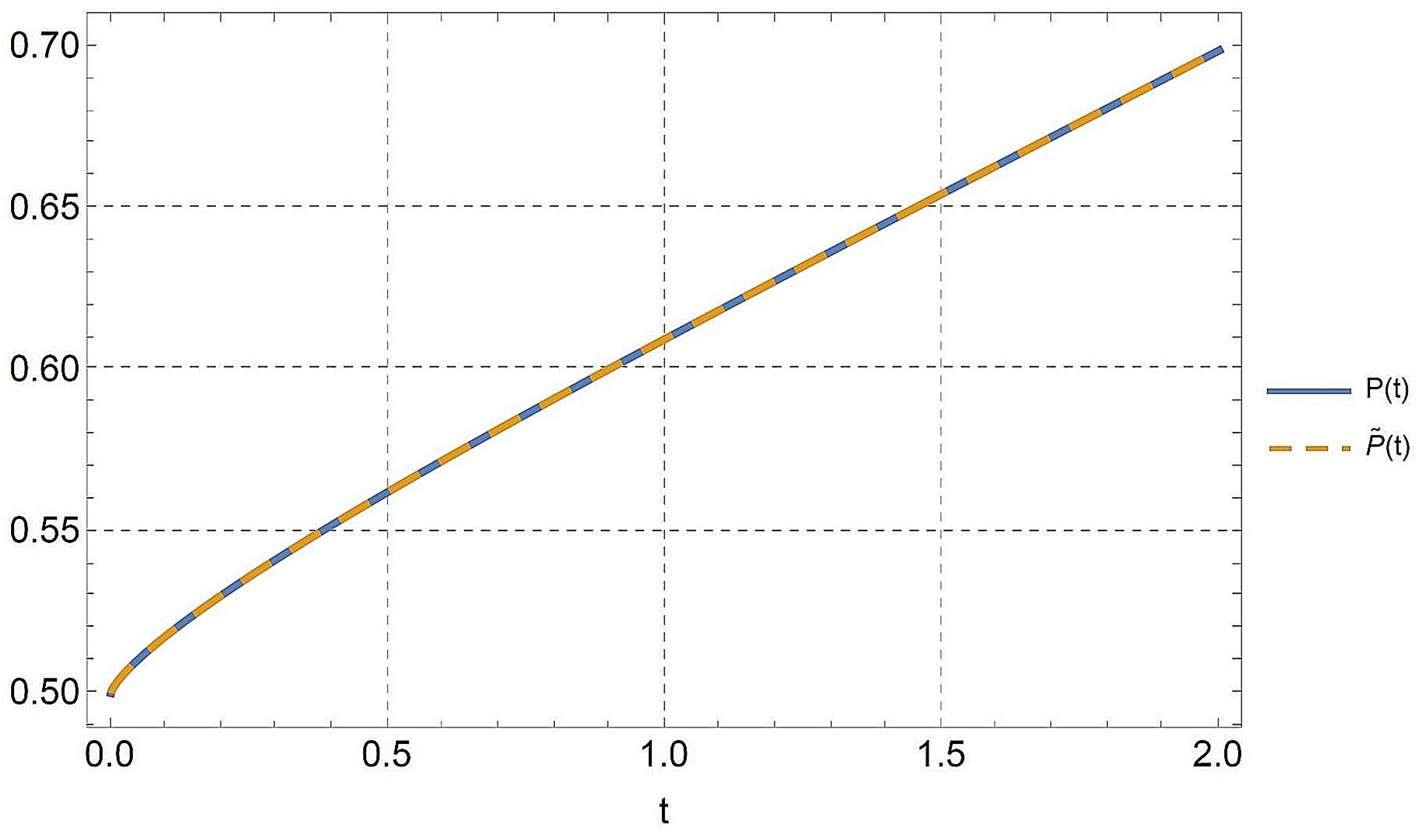
7.1.1. Example 7

Assuming that $\alpha =0.75;r=0.2;K=5.0;p_0=0.5$, and using the recursion in (27), we find the graph reported in Figure 1, where a comparison with the approximation obtained in [20] using the predictor-corrector method is shown.

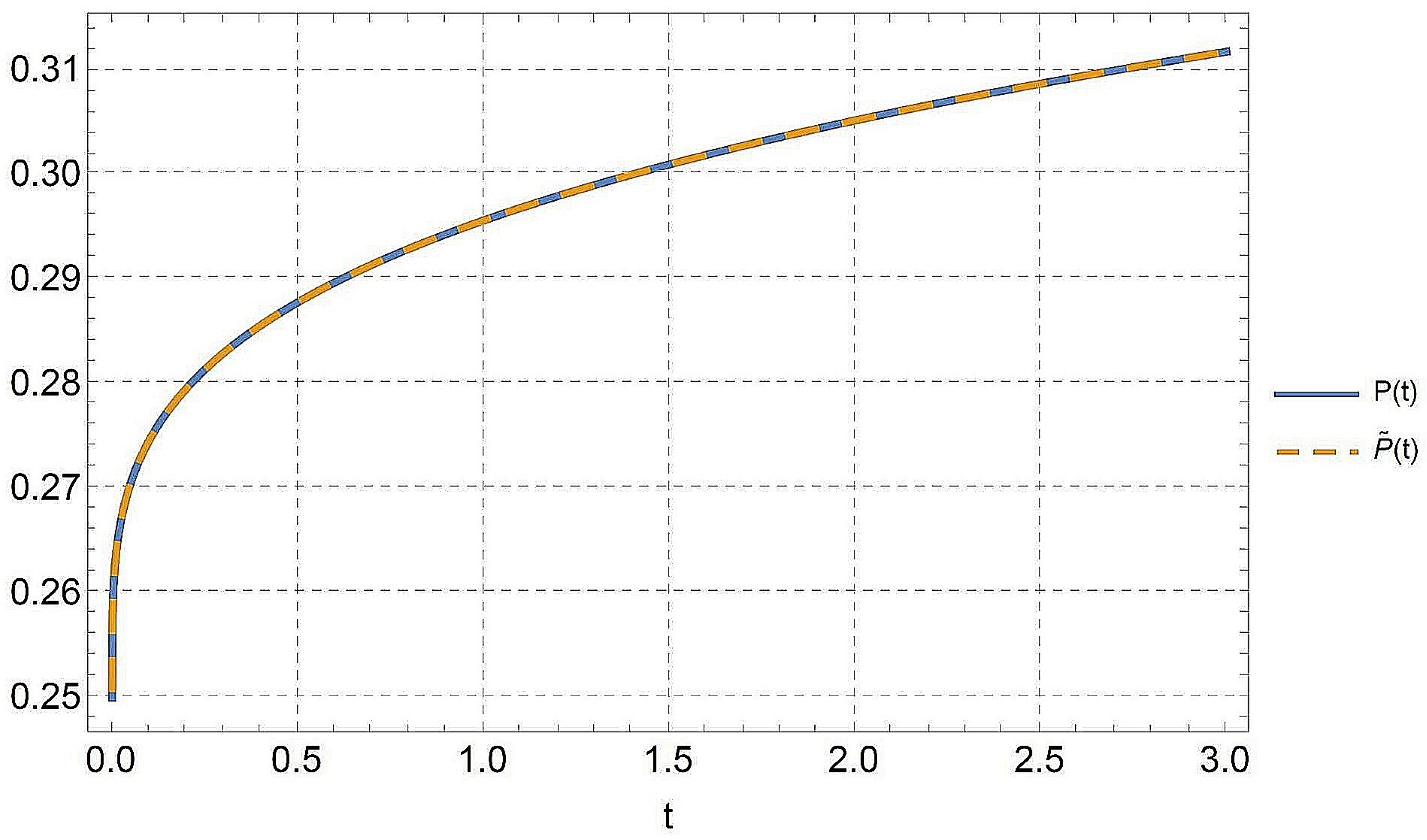
7.1.2. Example 8

Assuming that $\alpha =0.25;r=0.2;K=1.0;p_0=0.25$ and using the recursion in (27), we find the graph depicted in Figure 2, where a comparison with the approximation obtained in [20] using the predictor-corrector method is shown.

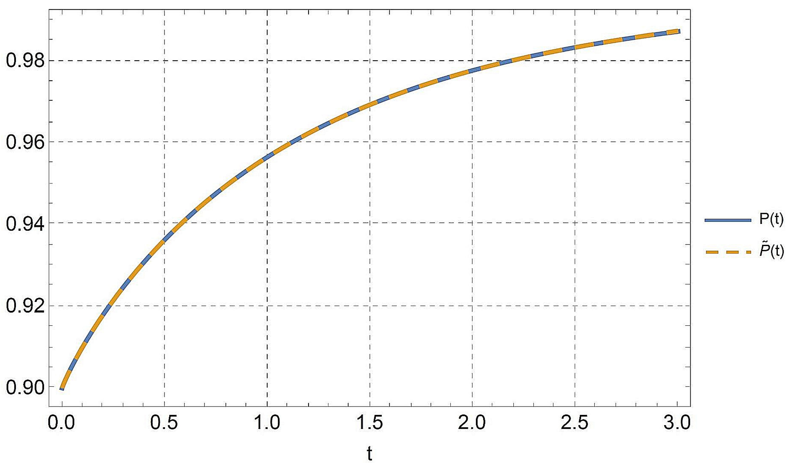
7.1.3. Example 9

Assuming that $\alpha =0.9;r=0.9;K=1.0;p_0=0.9$ and using the recursion in (27), we find the graph depicted in Figure 3, where a comparison with the approximation obtained in [20] using the predictor-corrector method is shown.

8. Conclusions

We have presented an elementary method to solve non-homogeneous fractional differential problems. The method is based on the series expansion of the solution in fractional powers with indeterminate coefficients. Using the classical Euler formula for fractional derivatives, which is part of the broader fractional differential operator theory introduced by Caputo, it is easy to construct the solution of initial value problems without resorting to more sophisticated theories.

An approximation of the solution for the fractional-order logistic equation has been provided, along with numerical verifications carried out using the Mathematica$\copyright$ computer algebra program.

We believe that this method could be extended to boundary value problems, though we have not yet verified such applications. However, we have considered the solution of more general initial problems in a recent article; see [17].

References

- Samko, S.; Kilbas, A.A.; Marichev, O. Fractional Integrals and Derivatives; Taylor & Francis: Abingdon, UK, 1993. [Google Scholar]
- Gorenflo, F.; Mainardi, F. Fractional Calculus: Integral and Differential Equations of Fractional Order. In Fractals and Fractional Calculus in Continuum Mechanics; Carpinteri, A., Mainardi, F., Eds.; Springer: New York, NY, USA, 1997; pp. 223–276. [Google Scholar]
- Mainardi, F.; Luchko, Y.; Pagnini, G. The fundamental solution of the space-time fractional diffusion equation. Fract. Calc. Appl. Anal. 2001, 4, 153–192. [Google Scholar]
- Abd-Elhameed, W.M.; Alsuyuti, M.M. Numerical Treatment of Multi-Term Fractional Differential Equations Via a New Kind of Generalized Chebyshev Polynomials. Fractal Fract. 2023, 7, 74. [Google Scholar] [CrossRef]
- Ford, N.J.; Connolly, J.A. Systems-based decomposition schemes for the approximate solution of multi-term fractional differential equations. J. Comput. Appl. Math. 2009, 229, 382–391. [Google Scholar] [CrossRef]
- Ghoreishi, F.; Yazdani, S. An extension of the spectral Tau method for numerical solution of multi-order fractional differential equations with convergence analysis. Comput. Math. Appl. 2011, 61, 30–43. [Google Scholar] [CrossRef]
- Jafari, S.D.H.; Tajadodi, H. Solving a multi-order fractional differential equation using homotopy analysis method. J. King Saud Univ. Sci. 2011, 23, 151–155. [Google Scholar] [CrossRef]
- Chen, Y.; Yi, M.; Yu, C. Error analysis for numerical solution of fractional differential equation by Haar wavelets method. J. Comput. Sci. 2012, 3, 367–373. [Google Scholar] [CrossRef]
- Seifollahi, M.; Shamloo, A. Numerical solution of nonlinear multi-order fractional differential equations by operational matrix of chebyshev polynomials. World Appl. Program. 2013, 3, 85–92. [Google Scholar] [CrossRef]
- Talaei, Y.; Asgari, M. An operational matrix based on Chelyshkov polynomials for solving multi-order fractional differential equations. Neural Comput. Appl. 2017, 30, 1369–1376. [Google Scholar] [CrossRef]
- Bonab, Z.F.; Javidi, M. Higher order methods for fractional differential equation based on fractional backward differentiation formula of order three. Math Comput Simul. 2020, 172, 71–89. [Google Scholar] [CrossRef]
- Hesameddini, E.; Rahimi, A.; Asadollahifard, E. On the convergence of a new reliable algorithm for solving multi-order fractional differential equations. Commun. Nonlinear Sci. Numer. Simul. 2015, 34, 154–164. [Google Scholar] [CrossRef]
- Groza, G.; Jianu, M. Functions represented into fractional Taylor series. In Proceedings of the 1st International Conference on Computational Methods and Applications in Engineering (ICCMAE 2018), Timisoara, Romania, 23–26 May 2018. [Google Scholar] [CrossRef]
- Ortigueira, M.D.; Trujillo, J.J.; Martynyuk, V.I.; Coito, F.J.V. A generalized power series and its application in the inversion of transfer functions. Signal Process. 2015, 107, 238–245. [Google Scholar] [CrossRef]
- Ortigueira, M.D. A New Look at the Initial Condition Problem. Mathematics 2022, 10, 1771. [Google Scholar] [CrossRef]
- Ortigueira, M.D.; Bengocheab, G. A new look at the fractionalization of the logistic equation. Physica A 2017, 467, 554–561. [Google Scholar] [CrossRef]
- Caratelli, D.; Natalini, P.; Ricci, P.E. Examples of expansions in fractional powers, and applications. Symmetry 2023, 15, 1702. [Google Scholar] [CrossRef]
- Beghin, L.; Caputo, M. Commutative and associative properties of the Caputo fractional derivative and its generalizing convolution operator. Commun. Nonlinear Sci. Numer. Simul. 2020, 89, 105338. [Google Scholar] [CrossRef]
- El-Sayed, A.M.A.; El-Mesiry, A.E.M.; El-Saka, H.A.A. On the fractional-order logistic equation. Appl. Math. Lett. 2007, 20, 817–823. [Google Scholar] [CrossRef]
- Diethelm, K.; Ford, N.J.; Freed, A.D. A Predictor-Corrector Approach for the Numerical Solution of Fractional Differential Equations. Nonlinear Dyn. 2002, 29, 3–22. [Google Scholar] [CrossRef]