Plane Wave Reflection in Nonlocal Semiconducting Rotating Media with Extended Model of Three-Phase-Lag Memory-Dependent Derivative

Abstract

The present paper examines the plane wave’s reflection in a semiconducting magneto-thermoelastic rotating nonlocal half-space medium, which is stress-free, thermally insulated, and with a diffusion transport process at the boundaries. The novel mathematical model of extended three-phase-lag (TPL) heat transfer law with memory-dependent derivative (MDD) and two temperatures (2T) is used to model this problem. The investigated 2D model shows that a longitudinal wave, when striking the surface z = 0, produces four reflected waves. The characteristics of the plane wave such as phase velocity, amplitude ratios, penetration depth, attenuation-coefficients-specific loss, and energy ratios of various reflected waves are obtained. The symmetric and asymmetric tensor representations of all physical quantities are used. The effects of various theories of thermoelasticity, two temperatures, and rotation on wave characteristics are illustrated graphically using MATLAB software.

1. Introduction

Many optical and microwave devices now use semiconductors that have very small dimensions and micro- and nanometer feature sizes to achieve higher frequencies and speeds, as well as denser circuits. In contrast to macrostructures, nanostructures exhibit significantly different wave properties as their dimensions decrease. The transmission of plane waves in a semiconductor thermoelastic solid has been seen as a promising material for solar cells, geophysics, nuclear fields, magnetometers, and allied topics. Therefore, the study of wave propagation is urgently needed.

Thermoelasticity is the study of the interactions between the mechanical and thermal forces in elastic bodies. Fractional thermoelasticity (FOT) theory was introduced by Sherief et al. [1] with fractional calculus, proving its theorem of uniqueness and deriving its variational principle and reciprocity theorems. The first generalized FOT model was developed by Povstenko [2] with the introduction of the classical thermoelasticity and generalized thermoelasticity of Green–Nagdhi (GN). In generalized heat conduction equations, Youssef [3] introduced Riemann–Liouville fractional integral operators, which result in generalized FOT. Ezzat et al. [4] used dual-phase-lag heat conduction laws in the fractional order (FO) in a mathematical model of two-temperature magneto-thermoelasticity. A generalized FOT was solved by Youssef and Abbas [5] based on FO thermal conductivity as a function of temperature. So far, we have discussed the following thermoelastic models:

• By applying Fourier law to thermoelasticity, Duhamel [6] developed the classical theory of thermoelasticity as $q_i=-K{T}_{,i},$ and heat conduction eqn. as: $\rho C_E\dot{T}=KT.$
• Catteno [7] and Vernotte [8] (CV) model: $q_i+\tau {\dot{q}}_i=-K{T}_{,i},$ and heat transport equation as $\rho C_E\left(\dot{T}+\tau \ddot{T}\right)=KT.$
• Green and Naghdi (GN) model [9,10,11]: ${\dot{q}}_i=-\left(K{\dot{T}}_{,i}+K*T_{,i}\right)$ gives $\rho C_E\ddot{T}=\left(K{\dot{T}}_{,i}+K*T_{,i}\right).$
• Dual-phase-lag (DPL) model [12,13]: $q_i+{\tau }_q{\dot{q}}_i+\frac{{\tau }_q^2}{2}{\ddot{q}}_i=-K\left(T_{,i}+{\tau }_T{\dot{T}}_{,i}\right),{\tau }_q>{\tau }_T>0.$
• Sherief et al. [1] fractional-order thermoelasticity (FOT) as $q_i+\tau \frac{{\partial }^{\alpha }}{\partial t^{\alpha }}{q}_i=-K{T}_{,i},\left(0<\alpha \le 1\right)$.
• Youssef [3] modified the CV heat conduction model by adding a fractional integral, as $q_i+\tau {\dot{q}}_i=-K{I}^{\alpha -1}{T}_{,i},\left(0<\alpha \le 2\right),$ where I indicates a Riemann–Liouville fractional integral operator defined as $I^{\alpha -1}f\left(t\right)=\frac{1}{\Gamma \left(\alpha -1\right)}{\int }_0^t{\left(t-\eta \right)}^{\alpha -2}f\left(\eta \right)d\eta , \mathrm{w}\mathrm{h}\mathrm{e}\mathrm{r}\mathrm{e} \Gamma \alpha$ is a gamma function).
• Using fractional Taylor’s series, Ezzat et al. [4] gave FOT as $q_i+\frac{{\tau }^{\alpha }}{\alpha }\frac{{\partial }^{\alpha }}{\partial t^{\alpha }}{q}_i=-K{T}_{,i},\left(0<\alpha \le 1\right).$

A superior MDD thermoelasticity model was proposed to illustrate the effect of memory (rate of unexpected change based on the previous state). It consists of a kernel function on a slip-in interval and is defined as an integral of a common derivative.

Recently, to define the memory dependence, Yu et al. [14] improved Lord–Shulman (LS) by introducing MDD into the rate of heat flux in generalized thermoelasticity theory as $\left(1+\eta D_{\eta }\right)q_i=-{ K}_{ij}{T}_{,i}, \left(0<\eta \le 1\right).$ Following Ezzat et al. [15], the memory-dependent derivatives from the Taylor theorem can be solved as

$$f\left(x,t+\chi \right)=f\left(x,t\right)+\sum _{n=1}^{\infty }\frac{{\eta }^n}{n!}{D}_{\eta }^{n}f\left(x,t\right),$$

where $n\in N,I:\left[a,b\right] \text{and} f:I\to R,$ since $f(x,t)$ and all derivatives are continuous on $I$ and $f^{n+1}\left(x,t\right)$ exist on $\left(a,b\right).$ Based on the Caputo-type fractional derivative, Wang and Li [16] proposed a novel derivative called MDD. If we compare the MDD with the fractional-order derivative, the MDD kernel function is selected based on real conditions, and its interval is not altered with time t. Moreover, it only depends on a restricted time period correlated with the past state $\left[t, t-\eta \right]$, where τ is known as the time delay. In addition to MDD, there exist numerous nonlocal theories, namely stress gradient theory [17], strain gradient theory [18], and many more. Based on the phonon dispersion test interpretations and molecular dynamics models, the nonlocal theory of elasticity exhibited better results compared with the classical theory of thermoelasticity. Nonlocal theory is used to define characteristics such as, if the size of any object reduces, it relates not only to the state of the present point but also to past time.

Using a plasma diffusion equation, Tang and Song [19] examined the reflection of waves in nonlocal semiconductor rotating media. Alshaikh [20] investigated the effects of diffusion and rotation on the transmission of photothermal waves through a semiconducting medium. Kaur et al. [21] investigated plane wave propagation in viscoelastic rotating media by using Hall current. The heat transfer and rotation of plane harmonic waves in the magneto-thermoelastic system were investigated with multi-dual-phase lags by Lata et al. [22]. In addition, researchers such as Jahangir et al. [23], Othman and Lotfy [24], Lata and Kaur [25], Taye et al. [26], Marin and Öchsner [27], Saeed et al. [28], Kiani et al. [29], Lotfy et al. [30], Ali et al. [31], Singh and Bijarnia [32], and Lotfy and Tantawi [33] have studied waves propagating in different media using different thermoelasticity theories.

In this paper, we study plane wave propagation in a nonlocal semiconducting rotating magneto-thermoelastic solid half-space, which is stress-free and thermally insulated, and has a diffusion transport process at the boundaries. A novel mathematical model of the extended TPL heat transfer law with MDD and 2T is used to model this problem. The effects of various theories of thermoelasticity, two temperatures, and rotation on wave characteristics are demonstrated graphically with MATLAB.

2. Basic Equations

As per Wang and Li [16], the 1st-order MDD with respect to time delay ${\eta }_i>0$, for a static time $t$ and an n times differentiable function $f\left(t\right)$:

$$D_{\eta }^{n}f\left(t\right)=\frac{1}{\eta }{\int }_{t-\eta }^{t}K\left(t-\eta \right)f^n\left(\eta \right)d\eta ,$$

(1)

where n is any natural number. The kernel function $K(t-\eta )$ is differentiable with respect to variables $t$ and $\eta$, which replicate the memory influence in the delay interval $[t-\eta , t],$ varying with time t and $0\le K(t-\eta )<1 \text{for} \eta \in [t-\eta , t].$ Also, the 1st- and 2nd-order MDD fulfill the relationship as

$$D_{\eta }^{2}f\left(t\right)=D{D}_{\eta }$$

The mth-order and 1st-order MDD satisfy the relationship as

$$D_{\eta }^{m}f\left(t\right)=\stackrel{m-1 times}{\overbrace{DDDD.....D}}{D}_{\omega },m\in N$$

where $D\equiv \frac{d}{dt}.$

The nonsingular kernel function $K(t-\eta )$, following Ezzat et al. [15,34,35], is given as

$$K\left(t-\eta \right)=1-\frac{2b}{\eta }\left(t-\eta \right)+\frac{c^2}{{\eta }^2}{\left(t-\eta \right)}^2=\left\{\begin{array}{c}1;\\ 1+\left(\eta -t\right)/\eta ;\\ \eta -t+1;\\ {\left[1+\left(\eta -t\right)/\eta \right]}^2;\end{array}\right.\begin{array}{c}c=0,b=0;\\ c=0,b=\raisebox{1ex}{$1$}\!\left/ \!\raisebox{-1ex}{$2$}\right.;\\ c=0,b=\raisebox{1ex}{$\eta $}\!\left/ \!\raisebox{-1ex}{$2$}\right.;\\ c=1,b=1;\end{array}$$

(2)

Following Kaur et al. [36] and Mahdy et al. [37], the MDD conduction equation with two temperatures irrespective of heat sources is given by

$$\begin{array}{c}{K}_{ij}\left(1+{\tau }_T{D}_{{\tau }_T}\right){\dot{\phi }}_{,ji}+K_{ij}^{*}\left(1+{\tau }_v{D}_{{\tau }_v}\right){\phi }_{,ji}-\frac{E_g}{\tau }\frac{\partial N\left(r,t\right)}{\partial t}=(1+{\tau }_q{D}_{{\tau }_q}+\\ \frac{{\tau }_q^2{D}_{{\tau }_q}^2}{2})\left[{\rho C}_E\ddot{T}+{\beta }_{ij}{T}_0{ё}_{ij}\right],\end{array}$$

(3)

$K_{ij}=K_i{\delta }_{ij},K_{ij}^{\mathrm{*}}=K_i^{\mathrm{*}}{\delta }_{ij};$ assuming that $K_{ij}$ is a symmetric tensor, $i$ is not summed.

Eringen [17] described, for a linear nonlocal thermoelastic solid, the equation of motion as

$$t_{ij,j}+f_i={\rho \ddot{u}}_i,$$

(4)

where

$$t_{ij}\left(x\right)={\int }_V\alpha \left(\left|x-x^{\mathrm{\prime }}\right|\right){\sigma }_{ij}\left(x^{\mathrm{\prime }}\right)dV\left(x^{\mathrm{\prime }}\right).$$

(5)

Now applying Equation (5) to Equation (4), the equivalent characteristic equations for a nonlocal anisotropic thermoelastic medium are obtained as

$$\left(1-ϵ{\nabla }^2\right)t_{ij}\left(x\right)={\sigma }_{ij}\left(x\right),$$

(6)

$$\mathrm{were}, ϵ=l^2{e}_0^2$$

(7)

$$t_{ij}-ϵ{\nabla }^2{t}_{ij}={\sigma }_{ij}\left(x\right).$$

(8)

The length in the macrostructures is comparatively less, i.e.,$ϵ=0,$ and hence Equation (6) is transformed into stress–strain identities of the classical theory of thermoelasticity. For the nonlocal kernel to be a Green function, the equation of motion is changed to

$${\sigma }_{ij,j}+\left(1-ϵ{\nabla }^2\right)f_i=\left(1-ϵ{\nabla }^2\right){\rho \ddot{u}}_i,$$

(9)

Following Othman and Abd-Elaziz [38], Tang and Song [19], and Eringen [39], utilizing the Lorentz force, the motion equations are

$$\begin{gathered} {\sigma }_{ij,j}+\left(1-{ϵ}^2{\nabla }^2\right) {\mu }_0{\epsilon }_{ijr}{J}_j{H}_r \\ =\rho \left(1-{ϵ}^2{\nabla }^2\right)\left\{{{\ddot{u}}_i+2{\left(\mathsf{\Omega }\times \dot{\mathit{u}}\right)}_i+\left(\mathsf{\Omega }\times (\mathsf{\Omega }\times \mathbf{u}\right))}_i\right\}, \end{gathered}$$

(10)

Here, a subscript $i$ tailed by ‘,’ indicates the partial derivative with respect to $x_i$, and a superposed dot signifies differentiation with respect to $t$. $\mathsf{\Omega }\times (\mathsf{\Omega }\times \mathbf{u})$ signifies centripetal acceleration, and $2\mathsf{\Omega }\times \dot{\mathit{u}}$ signifies the Coriolis acceleration.

Under a high magnetic field, the generalized Ohm’s law is modified with the presence of Hall current as

$$J_{\mathit{i}}+{\omega }_e{t}_e{\epsilon }_{ilk}{J}_l{H}_k={\sigma }_0\left(E_i+{\mu }_0{\epsilon }_{ijr}{\dot{u}}_j{H}_r\right),$$

(11)

where ${\omega }_e=\frac{e{\mu }_0{H}_0}{m_e}$ is the electron frequency. Following Lofty et al. [26], the stress–stress–strain–displacement–carrier density function equation is given by

$${\sigma }_{ij}=\left(\lambda u_{r,r}-\beta T-{\delta }_{n}N\right){\delta }_{ij}+\mu \left(u_{i,j}+u_{j,i}\right).$$

(12)

$$\mathrm{where} T=\phi -a{\phi }_{,ij},$$

(13)

$$\beta =\left(3\lambda +2\mu \right){\alpha }_T,$$

$${\delta }_n=\left(3\lambda +2\mu \right)d_n,$$

Here, a > 0 is the two-temperature parameter.

The plasma transference procedure in semiconductors is described by the plasma diffusion equation as

$$\frac{\partial N\left(r,t\right)}{\partial t}=D_E{\nabla }^{2}N\left(r,t\right)-\frac{N\left(r,t\right)}{\tau }+\kappa \frac{T}{\tau }.$$

(14)

3. Mathematical Modeling of the Problem

Consider a nonlocal semiconducting thermo-magnetoelastic homogeneous half-space that is rotating with an angular velocity $\mathsf{\Omega }=\left(0, \mathsf{\Omega }, 0\right)$ about the y-axis at a uniform temperature $T_0.$ We assume Cartesian coordinates $(x, y, z)$ with the origin on the surface $(z=0)$ and with the $z$-axis pointing into the medium. In 2D dynamic problems in the $xz$ plane, displacement vectors have the following form:

$$\mathit{u}=\left(u,0,w\right)\left(x,z,t\right).$$

(15)

For a very-high strength magnetic field, ${\mathit{H}}_0=(0, H_0, 0)$ is applied in the +positive y-direction. Thus

$$J_y=0.$$

(16)

and $J_x$ and $J_z$ are given as

$$J_x=\frac{{\sigma }_0{\mu }_0{H}_0}{1+m^2}\left(m\frac{\partial u}{\partial t}-\frac{\partial w}{\partial t}\right),$$

(17)

$$J_z=\frac{{\sigma }_0{\mu }_0{H}_0}{1+ m^{2 }}\left(\frac{\partial u}{\partial t}+m\frac{\partial w}{\partial t}\right).$$

(18)

Using Equations (15)–(18), in Equations (3), (10), and (14), the governing equations for nonlocal semiconducting medium with two temperatures are

$$\begin{array}{c}\left(\lambda +2\mu \right)\frac{{\partial }^{2}u}{\partial x^2}+\left(\lambda +\mu \right)\frac{{\partial }^{2}w}{\partial x\partial z}+\mu \frac{{\partial }^{2}u}{\partial z^2}-\beta \frac{\partial }{\partial x}\left\{\phi -a\left(\frac{{\partial }^2\phi }{\partial x^2}+\frac{{\partial }^2\phi }{\partial z^2}\right)\right\}-{\delta }_n\frac{\partial N}{\partial x}-\left(1-{ϵ}^2\left(\frac{{\partial }^2}{\partial x^2}+\frac{{\partial }^2}{\partial z^2}\right)\right)\frac{{\sigma }_0{\mu }_0^2{H}_0^2}{1+m^{2 }}(\frac{\partial u}{\partial t}+\\ m\frac{\partial w}{\partial t})=\rho \left(1-{ϵ}^2\left(\frac{{\partial }^2}{\partial x^2}+\frac{{\partial }^2}{\partial z^2}\right)\right)\left(\frac{{\partial }^{2}u}{\partial t^2}-{\Omega }^{2}u+2\Omega \frac{\partial w}{\partial t}\right),\end{array}$$

(19)

$$\begin{array}{c}\left(\lambda +\mu \right)\frac{{\partial }^{2}u}{\partial x\partial z}+\mu \frac{{\partial }^{2}w}{\partial x^2}+\left(\lambda +2\mu \right)\frac{{\partial }^{2}w}{\partial z^2}-\beta \frac{\partial }{\partial z}\left\{\phi -a\left(\frac{{\partial }^2\phi }{\partial x^2}+\frac{{\partial }^2\phi }{\partial z^2}\right)\right\}-{\delta }_n\frac{\partial N}{\partial z}+\left(1-{ϵ}^2\left(\frac{{\partial }^2}{\partial x^2}+\frac{{\partial }^2}{\partial z^2}\right)\right)\frac{{\sigma }_0{\mu }_0^2{H}_0^2}{1+ m^{2 }}(m\frac{\partial u}{\partial t}-\\ \frac{\partial w}{\partial t})=\rho \left(1-{ϵ}^2\left(\frac{{\partial }^2}{\partial x^2}+\frac{{\partial }^2}{\partial z^2}\right)\right)\left(\frac{{\partial }^{2}w}{\partial t^2}-{\Omega }^{2}w-2\Omega \frac{\partial u}{\partial t}\right),\end{array}$$

(20)

$$\frac{\partial N}{\partial t}=D_E\left(\frac{{\partial }^{2}N}{\partial x^2}+\frac{{\partial }^{2}N}{\partial z^2}\right)-\frac{N}{\tau }+\kappa \frac{T}{\tau },$$

(21)

$$\begin{array}{c}K\left(1+{\tau }_T{D}_{{\tau }_T}\right)\frac{\partial }{\partial t}\left(\frac{{\partial }^2\phi }{\partial x^2}+\frac{{\partial }^2\phi }{\partial z^2}\right)+K*\left(1+{\tau }_v{D}_{{\tau }_v}\right)\left(\frac{{\partial }^2\phi }{\partial x^2}+\frac{{\partial }^2\phi }{\partial z^2}\right)-\frac{E_g}{\tau }\frac{\partial N}{\partial t}=\left(1+{\tau }_q{D}_{{\tau }_q}+\frac{{\tau }_q^2{D}_{{\tau }_q}^2}{2}\right)\left[{\rho C}_E\frac{{\partial }^2}{\partial t^2}\right[\phi -\\ a\left(\frac{{\partial }^2\phi }{\partial x^2}+\frac{{\partial }^2\phi }{\partial z^2}\right)]+\beta T_0\frac{{\partial }^2}{\partial t^2}\left\{\frac{\partial u}{\partial x}+\frac{\partial w}{\partial z}\right\}],\end{array}$$

(22)

and

$${\sigma }_{xx}=\left(\lambda +2\mu \right)\frac{\partial u}{\partial x}+\lambda \frac{\partial w}{\partial z}-\beta T-{\delta }_{n}N,$$

(23)

$${\sigma }_{zz}=\lambda \frac{\partial u}{\partial x}+\left(\lambda +2\mu \right) \frac{\partial w}{\partial z}-\beta T-{\delta }_{n}N,$$

(24)

$${\sigma }_{xz}=\mu \left(\frac{\partial u}{\partial z}+\frac{\partial w}{\partial x}\right).$$

(25)

The dimensionless quantities are assumed by

$$\begin{array}{c}{(\tau }_T^{\prime }{,\tau }_v^{\prime },{\tau }_q^{\prime },t^{\prime })=\varpi *{(\tau }_T,{\tau }_v{,\tau }_q,t), c_1^2=\frac{\lambda +2\mu }{\rho },c_2^2=\frac{\mu }{\rho }, (x^{\prime },z^{\prime },u^{\prime },w^{\prime },{ϵ}^{\prime })=\frac{\varpi *}{c_1}(x,z,u,w,ϵ); T^{\prime }=\frac{\beta T}{\lambda +2\mu }{;\mathsf{\Omega }}^{\prime }=\\ \frac{1}{\varpi *}\mathsf{\Omega };({\sigma }_{xx}^{\prime },{\sigma }_{xz}^{\prime },{\sigma }_{zz}^{\prime })=\frac{1}{\lambda +2\mu }{(\sigma }_{xx},{\sigma }_{xz}{,\sigma }_{zz});a^{\prime }={\left(\frac{\varpi *}{c_1}\right)}^{2}a,{\phi }^{\prime }=\frac{\beta \phi }{\lambda +2\mu },\left({\varphi }^{\prime },{\psi }^{\prime }\right)={\left(\frac{\varpi *}{c_1}\right)}^2\left(\varphi ,\psi \right),N^{\prime }=\frac{{\delta }_{n}N}{\lambda +2\mu },\varpi *=\\ \frac{\rho C_E{c}_1^2}{K},{\delta }^2=\frac{c_2^2}{c_1^2},M=\frac{{\sigma }_0{\mu }_0^2{H}_0^2}{\rho \varpi *}.\end{array}$$

(26)

Using (26) in Equations (19)–(22), after suppressing the primes, yields

$$\begin{array}{c}\frac{{\partial }^{2}u}{\partial x^2}+\left(1-{\delta }^2\right)\frac{{\partial }^{2}w}{\partial x\partial z}+{\delta }^2\frac{{\partial }^{2}u}{\partial z^2}-\frac{\partial }{\partial x}\left\{\phi -a\left(\frac{{\partial }^2\phi }{\partial x^2}+\frac{{\partial }^2\phi }{\partial z^2}\right)\right\}-\frac{\partial N}{\partial x}=(1-\\ {ϵ}^2\left(\frac{{\partial }^2}{\partial x^2}+\frac{{\partial }^2}{\partial z^2}\right))\left\{\frac{M}{1+m^2}\left[\frac{\partial u}{\partial t}+m\frac{\partial w}{\partial t}\right]+\left(\frac{{\partial }^{2}u}{\partial t^2}-{\mathsf{\Omega }}^{2}u+2\mathsf{\Omega }\frac{\partial w}{\partial t}\right)\right\},\end{array}$$

(27)

$$\begin{array}{c}\left(1-{\delta }^2\right)\frac{{\partial }^{2}u}{\partial x\partial z}+{\delta }^2\frac{{\partial }^{2}w}{\partial x^2}+\frac{{\partial }^{2}w}{\partial z^2}-\frac{\partial }{\partial z}\left\{\phi -a\left(\frac{{\partial }^2\phi }{\partial x^2}+\frac{{\partial }^2\phi }{\partial z^2}\right)\right\}-\frac{\partial N}{\partial z}=(1-\\ {ϵ}^2\left(\frac{{\partial }^2}{\partial x^2}+\frac{{\partial }^2}{\partial z^2}\right))\left\{\frac{-M}{1+m^2}\left[m\frac{\partial u}{\partial t}-\frac{\partial w}{\partial t}\right]+\left(\frac{{\partial }^{2}w}{\partial t^2}-{\mathsf{\Omega }}^{2}w-2\mathsf{\Omega }\frac{\partial u}{\partial t}\right)\right\},\end{array}$$

(28)

$$\left[\left(\frac{{\partial }^2}{\partial x^2}+\frac{{\partial }^2}{\partial z^2}\right)-{\delta }_1\left(\frac{\partial }{\partial t}+{\delta }_2\right)\right]N+{\epsilon }_3\left\{\phi -a\left(\frac{{\partial }^2\phi }{\partial x^2}+\frac{{\partial }^2\phi }{\partial z^2}\right)\right\}=0,$$

(29)

$$\begin{array}{c}\left(1+{\tau }_T{D}_{{\tau }_T}\right)\frac{\partial }{\partial t}\left(\frac{{\partial }^2\phi }{\partial x^2}+\frac{{\partial }^2\phi }{\partial z^2}\right)+\frac{K*}{K\varpi *}\left(1+{\tau }_v{D}_{{\tau }_v}\right)\left(\frac{{\partial }^2\phi }{\partial x^2}+\frac{{\partial }^2\phi }{\partial z^2}\right)+{\epsilon }_2\frac{\partial N}{\partial t}=\\ \left(1+{\tau }_q{D}_{{\tau }_q}+\frac{{\tau }_q^2{D}_{{\tau }_q}^2}{2}\right)\left[\frac{{\partial }^2}{\partial t^2}\left\{\phi -a\left(\frac{{\partial }^2\phi }{\partial x^2}+\frac{{\partial }^2\phi }{\partial z^2}\right)\right\}+{\epsilon }_1\left\{\frac{\partial \ddot{u}}{\partial x}+\frac{\partial \ddot{w}}{\partial z}\right\}\right],\end{array}$$

(30)

where

$${\delta }_1=\frac{c_1^2}{D_E\varpi *},{\epsilon }_3=\frac{\kappa K{d}_n}{{\alpha }_T\rho C_E{D}_E\varpi *\tau \prime },{\epsilon }_2=\frac{E_g{\alpha }_T}{d_n\rho C_E{\left(\varpi *\right)}^2\tau \prime },{\epsilon }_1=\frac{{\beta }^2{T}_0}{\rho C_E\left(\lambda +2\mu \right)},{\delta }_2=\frac{1}{\tau }$$

The parameter ${\mathsf{\epsilon }}_1$ is governed by specific heat, temperature ${\mathrm{T}}_0$, and Lame’s elastic constants, and ${\mathsf{\epsilon }}_3$ is determined by the electronic deformation coefficient ${\mathrm{d}}_n$ using (26) in Equations (23)–(25), after omitting the primes, yields.

$${\sigma }_{\mathrm{x}\mathrm{x}}\left(\mathrm{x},\mathrm{z},\mathrm{t}\right)=\frac{\partial u}{\partial x}+\left(1-2{\delta }^2\right)\frac{\partial w}{\partial z}-\left\{\phi -a\left(\frac{{\partial }^2\phi }{{\partial x}^2}+\frac{{\partial }^2\phi }{{\partial z}^2}\right)\right\}-N,$$

(31)

$${\sigma }_{\mathrm{z}\mathrm{z}}\left(\mathrm{x},\mathrm{z},\mathrm{t}\right)=\left(1-2{\delta }^2\right)\frac{\partial u}{\partial x}+\frac{\partial w}{\partial z}-\left\{\phi -a\left(\frac{{\partial }^2\phi }{{\partial x}^2}+\frac{{\partial }^2\phi }{{\partial z}^2}\right)\right\}-N,$$

(32)

$${\sigma }_{\mathrm{x}\mathrm{z}}(\mathrm{x},\mathrm{z},\mathrm{t})={\delta }^2\left(\frac{\partial u}{\partial z}+\frac{\partial w}{\partial x}\right),$$

(33)

The potential functions $\varphi$ and $\psi$ are represented as

$$u=\frac{\partial \varphi }{\partial x}-\frac{\partial \psi }{\partial z}, w=\frac{\partial \varphi }{\partial z}+\frac{\partial \psi }{\partial x},e={\nabla }^2\varphi ,\frac{\partial w}{\partial x}-\frac{\partial u}{\partial z}={\nabla }^2\psi ,$$

(34)

Using (25) in Equations (18)–(21) yields

$$\begin{array}{c}{\delta }^2{\nabla }^2\psi +\left\{\phi -a{\nabla }^2\phi \right\}+N=\left(1-{ϵ}^2{\nabla }^2\right)\{\frac{M}{1+m^2}\left[\frac{\partial \psi }{\partial t}-m\frac{\partial \varphi }{\partial t}\right]+(\frac{{\partial }^2\psi }{\partial t^2}-{\mathsf{\Omega }}^2\psi -\\ 2\mathsf{\Omega }\frac{\partial \varphi }{\partial t}\left)\right\},\end{array}$$

(35)

$${\nabla }^2\varphi =\left(1-{ϵ}^2{\nabla }^2\right)\left\{\frac{M}{1+m^2}\left[m\frac{\partial \psi }{\partial t}+\frac{\partial \varphi }{\partial t}\right]+\left(\frac{{\partial }^2\varphi }{\partial t^2}-{\mathsf{\Omega }}^2\varphi +2\mathsf{\Omega }\frac{\partial \psi }{\partial t}\right)\right\},$$

(36)

$$\left[{\nabla }^2-{\delta }_1\left(\frac{\partial }{\partial t}+{\delta }_2\right)\right]N+{\epsilon }_3\left\{\phi -a{\nabla }^2\phi \right\}=0,$$

(37)

$$\begin{array}{c}\left\{\left(1+{\tau }_T{D}_{{\tau }_T}\right)\frac{\partial }{\partial t}+\frac{K*}{K\varpi *}\left(1+{\tau }_v{D}_{{\tau }_v}\right)\right\}{\nabla }^2\phi +{\epsilon }_{2}N\\ \hspace{1em}\hspace{1em}\hspace{1em}\hspace{1em}\hspace{1em}\hspace{1em}\hspace{1em}\hspace{1em}\hspace{1em}\hspace{1em}\hspace{1em}\hspace{1em}\hspace{1em}\hspace{1em}\hspace{1em}\hspace{1em}=\left(1+{\tau }_q{D}_{{\tau }_q}+\frac{{\tau }_q^2{D}_{{\tau }_q}^2}{2}\right)\left[\frac{{\partial }^2}{\partial t^2}\left\{\phi -a{\nabla }^2\phi \right\}+{\epsilon }_1\frac{{\partial }^2}{{\partial t}^2}{\nabla }^2\varphi \right],\end{array}$$

(38)

where

$${\nabla }^2\equiv \frac{{\partial }^2}{{\partial x}^2}+\frac{{\partial }^2}{{\partial z}^2}.$$

The stress–strain relationships become

$${\sigma }_{\mathrm{x}\mathrm{x}}\left(\mathrm{x},\mathrm{z},\mathrm{t}\right)=\frac{{\partial }^2\varphi }{\partial x^2}+\left(1-2{\delta }^2\right)\frac{{\partial }^2\varphi }{\partial z^2}-2{\delta }^2\frac{{\partial }^2\psi }{\partial x\partial z}-\left\{\phi -a{\nabla }^2\right\}-N$$

(39)

$${\sigma }_{\mathrm{z}\mathrm{z}}\left(\mathrm{x},\mathrm{z},\mathrm{t}\right)=\left(1-2{\delta }^2\right)\frac{{\partial }^2\varphi }{\partial x^2}+\frac{{\partial }^2\varphi }{\partial z^2}+2{\delta }^2\left(\frac{{\partial }^2\psi }{\partial x\partial z}\right)-\left\{\phi -a{\nabla }^2\right\}-N,$$

(40)

$${\sigma }_{\mathrm{x}\mathrm{z}}(\mathrm{x},\mathrm{z},\mathrm{t})={\delta }^2\left(2\frac{{\partial }^2\varphi }{\partial x\partial z}-\frac{{\partial }^2\psi }{\partial z^2}+\frac{{\partial }^2\psi }{\partial x^2}\right),$$

(41)

For the solution of the Equations (35)–(38), we assume that

$$\left(\begin{array}{c}\varphi \\ \psi \\ \phi \\ N\end{array}\right)=\left(\begin{array}{c}\overline{\varphi }\\ \overline{\psi }\\ \overline{\phi }\\ \overline{N}\end{array}\right)e^{\left(i\xi (x sin\theta +z cos\theta \right)-i\omega t)},$$

(42)

where $sin\theta , cos\theta$ is the projection of the wave that is normal to the $x-z$ plane; $i=\sqrt{-1}, \mathrm{a}\mathrm{n}\mathrm{d} \overline{\varphi },\overline{\psi },\overline{\phi },\mathrm{a}\mathrm{n}\mathrm{d} \overline{N}$ are the undetermined constants.

Using Equation (42) in Equations (35)–(38) yields

$$\left[{\zeta }_2+{\zeta }_4{\xi }^2\right]\overline{\varphi }+\left[{\zeta }_1{+\zeta }_3{\xi }^2\right]\overline{\psi }+\left[1+a{\xi }^2\right]\overline{\phi }+\overline{N}=0,$$

(43)

$$\left[{\zeta }_6{\xi }^2+{\zeta }_5\right]\overline{\varphi }+\left[{\zeta }_8{\xi }^2+{\zeta }_7\right]\overline{\psi }-=0,$$

(44)

$${\epsilon }_3\left[1+a{\xi }^2\right]\overline{\phi }+\left[{\zeta }_9-{\xi }^2\right]\overline{N}=0,$$

(45)

$${\zeta }_{13}{\xi }^2\overline{\varphi }+\left[{\zeta }_{12}{\xi }^2+{\zeta }_{10}\right]\overline{\phi }+{\epsilon }_{2}i\omega \overline{N}=0.$$

(46)

Additionally, the stress–strain equation is expressed as

$${\sigma }_{xx}=\left[-{\xi }^2\left({sin}^2\theta +\left(1-2{\delta }^2\right){cos}^2\theta \right)\overline{\varphi }-{\xi }^2\left({\delta }^2\right)\sin 2\theta \overline{\psi }-\left[1+a{\xi }^2\right]\overline{\phi }-\overline{N}\right]e^{\left(i\xi (x sin\theta +z cos\theta \right)-i\omega t)}$$

(47)

$${\sigma }_{\mathrm{z}\mathrm{z}}=\left[-{\xi }^2\left(\left(1-2{\delta }^2\right){sin}^2\theta +{cos}^2\theta \right)\overline{\varphi }-{\xi }^2\left({\delta }^2\right)\sin 2\theta \overline{\psi }-\left[1+a{\xi }^2\right]\overline{\phi }-\overline{N}\right]e^{\left(i\xi (x sin\theta +z cos\theta \right)-i\omega t)},$$

(48)

$${\sigma }_{\mathrm{x}\mathrm{z}}(\mathrm{x},\mathrm{z},\mathrm{t})=-{\xi }^2{\delta }^2\left(\sin 2\theta \overline{\varphi }-\cos 2\theta \overline{\psi }\right)e^{\left(i\xi (x sin\theta +z cos\theta \right)-i\omega t)},$$

(49)

where, ${\zeta }_1=\left(\frac{i\omega M}{1+m^2}+{\omega }^2+{\mathsf{\Omega }}^2\right),$

$${\zeta }_2=-\left(\frac{Mmi\omega }{1+m^2}+2\omega \mathsf{\Omega }i\right),$$

$${\zeta }_3={\zeta }_1{ϵ}^2-{\delta }^2,$$

$${\zeta }_4={\zeta }_2{ϵ}^2,$$

$${\zeta }_5=\frac{Mi\omega }{1+m^2}+{\omega }^2+{\mathsf{\Omega }}^2,$$

$${\zeta }_6={\zeta }_5{ϵ}^2-1,$$

$${\zeta }_7=\frac{Mmi\omega }{1+m^2}+2\omega \mathsf{\Omega }i,$$

$${\zeta }_8={\zeta }_7{ϵ}^2,$$

$${\zeta }_9={\delta }_1\left(i\omega -{\delta }_2\right),$$

$${\zeta }_{10}=\left(1+{\tau }_q{G}_{{\tau }_q}+\frac{{\tau }_q^2{G}_{{\tau }_q}^2}{2}\right){\omega }^2,$$

$${\zeta }_{11}=\left(1+{\tau }_T{G}_{{\tau }_T}\right) i\omega -\frac{K*}{K\omega *}\left(1+{\tau }_v{G}_{{\tau }_v}\right),$$

$${\zeta }_{13}=-{\zeta }_{10}{\epsilon }_1,$$

$${\zeta }_{12}=\left({\zeta }_{11}-{\zeta }_{10}a\right) .$$

$$G_{{\tau }_j}=\frac{i}{\omega }\left\{\frac{\left(1-e^{i\omega {\tau }_j}\right)i}{\omega {\tau }_j}-2b\left[\frac{\left(1-i\omega {\tau }_j\right)e^{i\omega {\tau }_j}-1}{{\left(\omega {\tau }_j\right)}^2}\right]+c^2\left[\frac{\left(i\left({\left(\omega {\tau }_j\right)}^2-2\right)-2\tau \omega \right)e^{i\omega {\tau }_j}-2i}{{\left(\omega {\tau }_j\right)}^3}\right]\right\}$$

$$G_{{\tau }_j}^2=\frac{i}{\omega }{G}_{{\tau }_j}$$

where $j$ takes values $T,v,q$.

For the nontrivial solution of Equations (43)–(46), the determinant of the coefficients of $\overline{\varphi },\overline{\psi }, \overline{\phi }$, and $\overline{N}$ must vanish, resulting in the characteristic equation

$$A{\xi }^8+B{\xi }^6+C{\xi }^4+D{\xi }^2+E=0,$$

(50)

where

$$A=-{\zeta }_{13}{\zeta }_9{\zeta }_{8}a+{\zeta }_{12}{\zeta }_4{\zeta }_8-{\zeta }_3{\zeta }_6{\zeta }_{12} ,$$

$$\begin{array}{c}B=-a{\epsilon }_3{\zeta }_{13}{\zeta }_8+{\epsilon }_{2}i\omega {\epsilon }_3{\zeta }_4{\zeta }_{8}a-a{\epsilon }_{2}i\omega {\epsilon }_3{\zeta }_6{\zeta }_3-{\zeta }_{13}{\zeta }_9{\zeta }_{7}a+{\zeta }_{13}{\zeta }_9{\zeta }_{8}a-{\zeta }_{13}{\zeta }_9{\zeta }_8+\\ {\zeta }_{12}{\zeta }_2{\zeta }_8-{\zeta }_1{\zeta }_6{\zeta }_{12}-{\zeta }_{12}{\zeta }_9{\zeta }_4{\zeta }_8+{\zeta }_{10}{\zeta }_4{\zeta }_8+{\zeta }_{12}{\zeta }_9{\zeta }_6{\zeta }_3-{\zeta }_3{\zeta }_6{\zeta }_{10}+{\zeta }_{12}{\zeta }_4{\zeta }_7-\\ {\zeta }_{12}{\zeta }_5{\zeta }_3,\end{array}$$

$$\begin{array}{c}C={\zeta }_{13}{\zeta }_9{\zeta }_8+{\zeta }_{13}{\zeta }_9{\zeta }_{7}a-{\zeta }_{13}{\zeta }_9{\zeta }_7-{\epsilon }_3{\zeta }_{13}{\zeta }_8-{\epsilon }_3{\zeta }_{13}{\zeta }_7+{\epsilon }_{2}i\omega {\epsilon }_3{\zeta }_4{\zeta }_8-\\ {\epsilon }_{2}i\omega {\epsilon }_3{\zeta }_6{\zeta }_3+\left({\epsilon }_2{\epsilon }_3{\zeta }_2{\zeta }_8+{\epsilon }_2{\epsilon }_3{\zeta }_4{\zeta }_7-{\epsilon }_2{\epsilon }_3{\zeta }_6{\zeta }_1-{\epsilon }_2{\epsilon }_3{\zeta }_5{\zeta }_3\right)ai\omega -{\zeta }_{12}{\zeta }_9{\zeta }_2{\zeta }_8+\\ {\zeta }_{10}{\zeta }_2{\zeta }_8+{\zeta }_{12}{\zeta }_6{\zeta }_1{\zeta }_9-{\zeta }_{10}{\zeta }_1{\zeta }_6-{\zeta }_{10}{\zeta }_9{\zeta }_4{\zeta }_8-{\zeta }_{12}{\zeta }_5{\zeta }_1+{\zeta }_{12}{\zeta }_2{\zeta }_7-{\zeta }_{12}{\zeta }_4{\zeta }_7{\zeta }_9+\\ {\zeta }_{10}{\zeta }_4{\zeta }_7+{\zeta }_{12}{\zeta }_9{\zeta }_5{\zeta }_3-{\zeta }_{10}{\zeta }_5{\zeta }_3,\end{array}$$

$$\begin{array}{c}D={\zeta }_{13}{\zeta }_9{\zeta }_7-{\epsilon }_3{\zeta }_{13}{\zeta }_7+({\epsilon }_2{\epsilon }_3{\zeta }_2{\zeta }_8+{\epsilon }_2{\epsilon }_3{\zeta }_4{\zeta }_7-\\ {\epsilon }_2{\epsilon }_3{\zeta }_6{\zeta }_1-{\epsilon }_2{\epsilon }_3{\zeta }_5{\zeta }_3+a{\epsilon }_2{\epsilon }_3{\zeta }_2{\zeta }_7-a{\epsilon }_2{\epsilon }_3{\zeta }_5{\zeta }_1)i\omega -\\ {\zeta }_{10}{\zeta }_9{\zeta }_2{\zeta }_8+{\zeta }_{10}{\zeta }_9{\zeta }_1{\zeta }_6+{\zeta }_{12}{\zeta }_9{\zeta }_5{\zeta }_1-{\zeta }_{10}{\zeta }_1{\zeta }_5+{\zeta }_{10}{\zeta }_7{\zeta }_2-\\ {\zeta }_{10}{\zeta }_9{\zeta }_4{\zeta }_7+{\zeta }_{10}{\zeta }_9{\zeta }_3{\zeta }_5,\\ E=\left({\epsilon }_2{\epsilon }_3{\zeta }_2{\zeta }_7-{\epsilon }_2{\epsilon }_3{\zeta }_5{\zeta }_1\right)i\omega +{\zeta }_{10}{\zeta }_9{\zeta }_5{\zeta }_1-{\zeta }_{12}{\zeta }_9{\zeta }_2{\zeta }_7-{\zeta }_{10}{\zeta }_9{\zeta }_2{\zeta }_7+{\zeta }_{10}{\zeta }_9{\zeta }_3{\zeta }_6.\end{array}$$

The solution of Equation (50) gives eight roots in $\xi$ that is, $\pm {\xi }_1, {\pm \xi }_2,{\pm \xi }_3,{\pm \xi }_4,$ and we are apprehensive with the positive imaginary parts of the roots. It shows that the produced waves are coupled in nature. Four reflected waves are produced when a longitudinal wave hits a surface with z = 0.

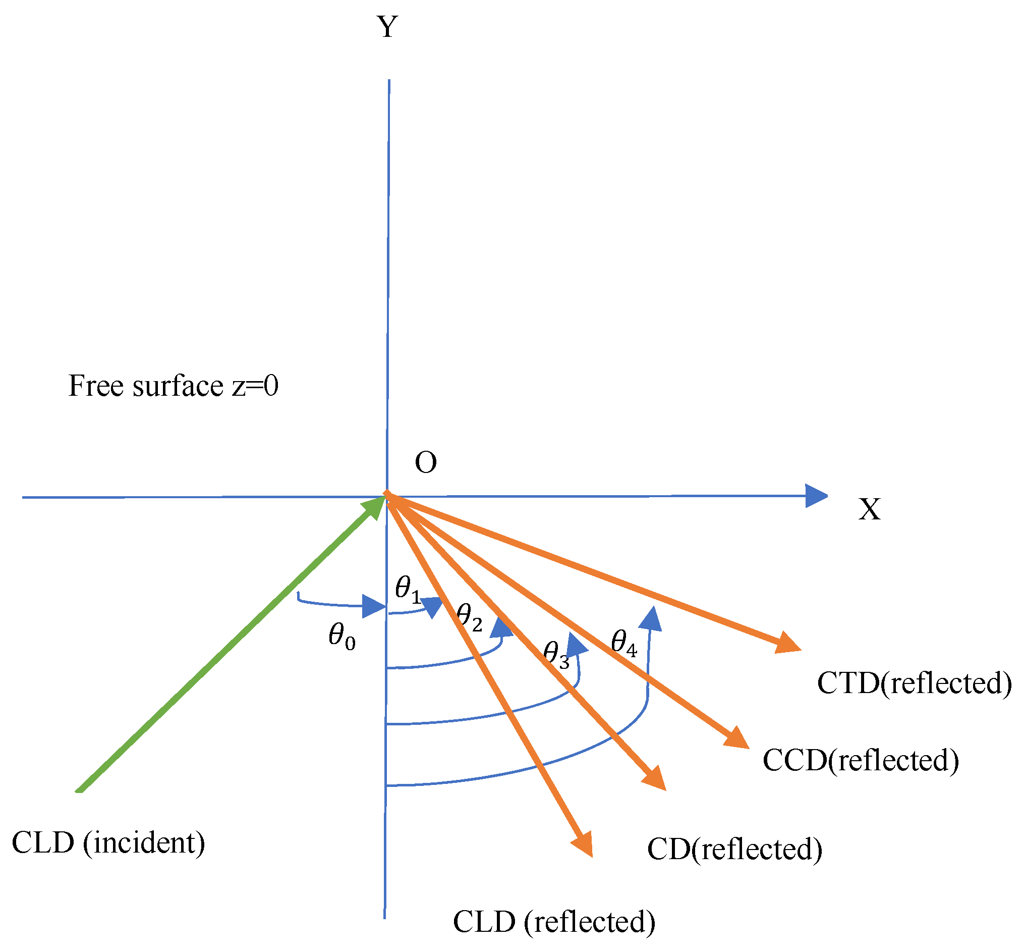
4. Reflection at the Free Boundary Surfaces

Consider a semiconducting magneto-thermoelastic homogeneous half-space occupying the region $z \ge 0$, with thermally insulated and stress-free surface $z=0$. It is theoretically investigated when a longitudinal CLD wave with an angle ${\mathit{\theta }}_0$ with the normal striking the surface $z=0$ results in the four coupled CLD, CD, CCD, and CTD reflected waves through the medium $z\ge 0$ as shown in Figure 1.

At z = 0, the generalized Snell’s law is defined as follows:

$${\xi }_{0}sin{\theta }_0={\xi }_{1}sin{\theta }_1={\xi }_{2}sin{\theta }_2={\xi }_{3}sin{\theta }_3={\xi }_{4}sin{\theta }_4$$

(51)

where $subscripts 1, 2, 3, 4$ represent the quantities for reflected waves, and $subscript 0$ represents the incident wave. You can figure out the direction of the wave reflection’s attenuation and propagation by using

$${\theta }_j={\sin }^{-1}\left(\frac{V_j}{V_0}\sin {\theta }_0\right),j=1,2,3,4.$$

(52)

Four coupled waves are now identified, with the CLD wave associated with the maximum speed of transmission ${\mathrm{V}}_1$, the CT wave associated with the second-fastest speed of transmission ${\mathrm{V}}_2$, the CCD wave associated with the third-fastest speed of transmission ${\mathrm{V}}_3$, and the CTD wave associated with the slowest transmission ${\mathrm{V}}_4$, all of which correspond to the four positive roots. The features of these waves are characterized by the following expressions:

(i) Phase velocity

We can determine phase velocities as follows:

$$V_j=\frac{\omega }{Re\left({\xi }_j\right)},j=1,2,3,4$$

According to this equation,${ V}_1, V_2, V_3, \mathrm{a}\mathrm{n}\mathrm{d} V_4$ represent the CLD, CT, CCD, and CTD waves phase velocities, respectively, and $Re\left({\xi }_j\right)$ means the real part of ${\xi }_j.$

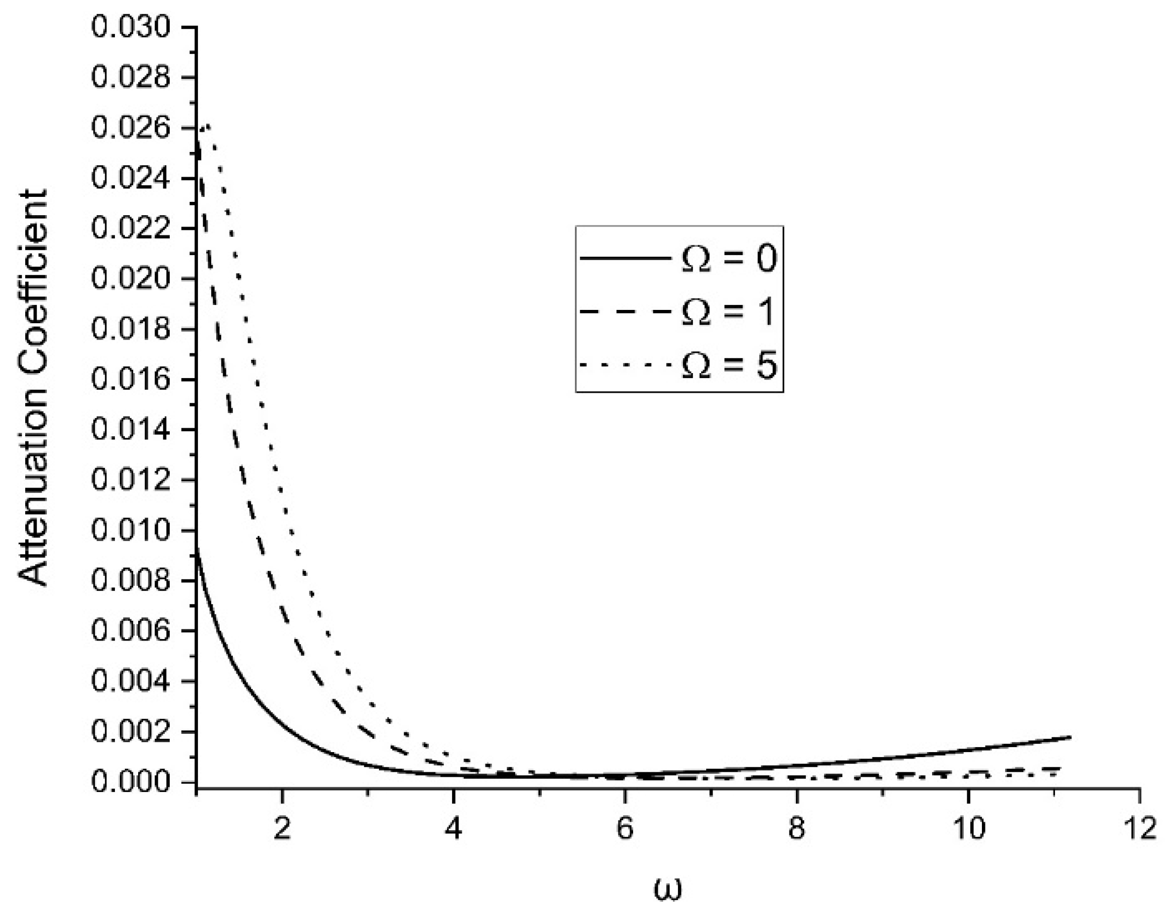
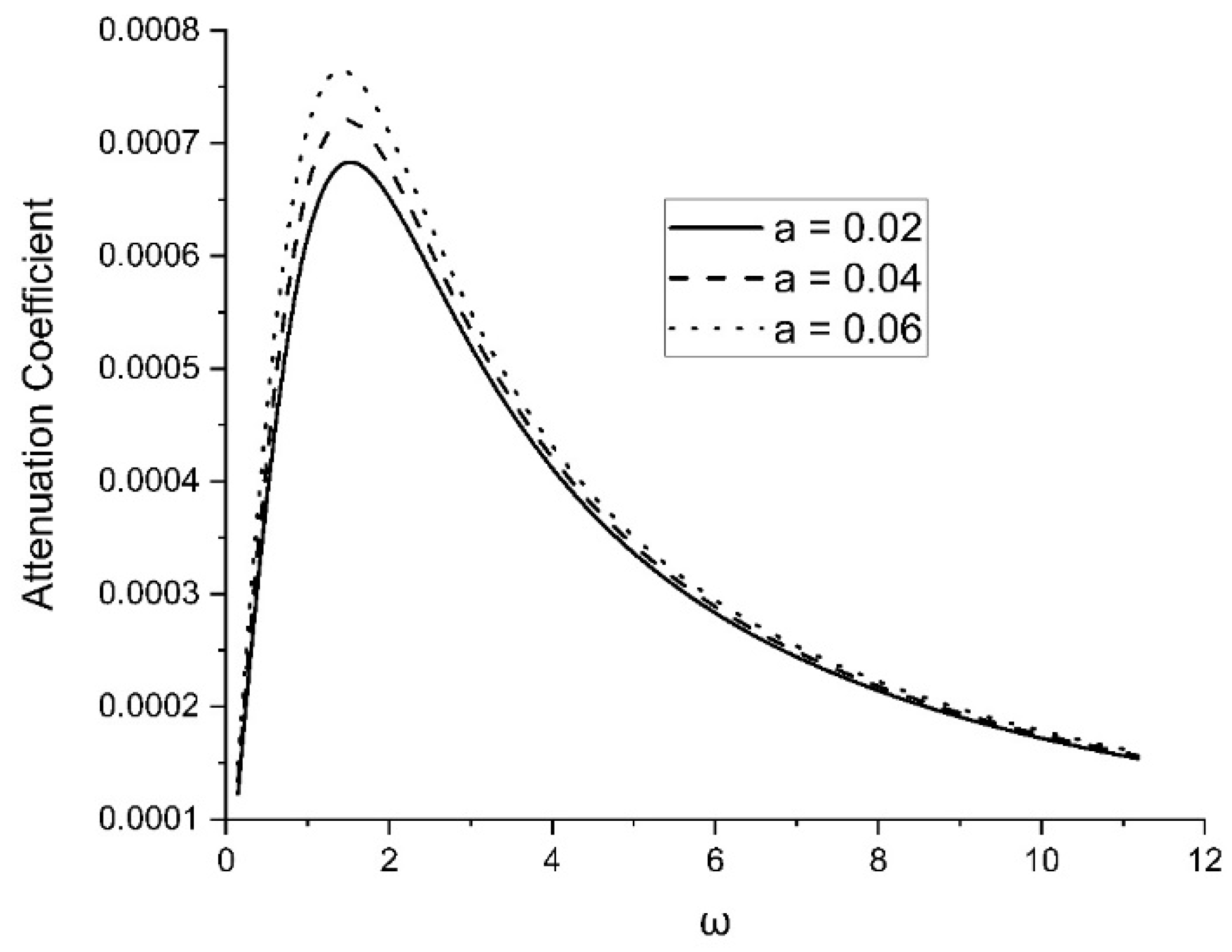
(ii) Attenuation Coefficient

We can determine the attenuation coefficient as follows:

$$Q_j=Img\left({\xi }_j\right),j=1,2,3,4.$$

where $Q_1, Q_2, Q_3, \mathrm{a}\mathrm{n}\mathrm{d} Q_4$ represent the CLD, CT, CCD, and CTD wave attenuation coefficients, respectively, and $Img\left({\xi }_j\right)$ means the imaginary part of $\left({\xi }_j\right)$.

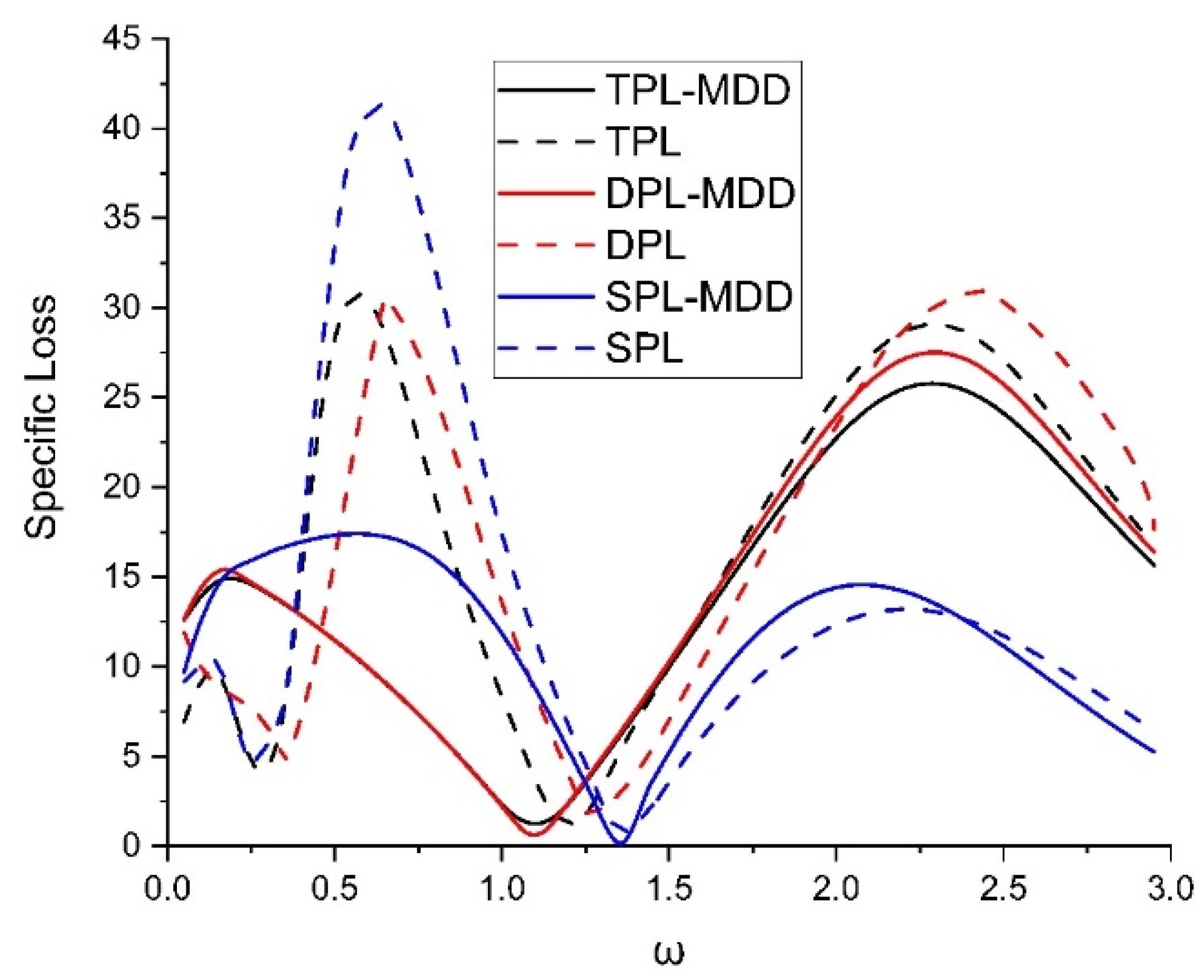
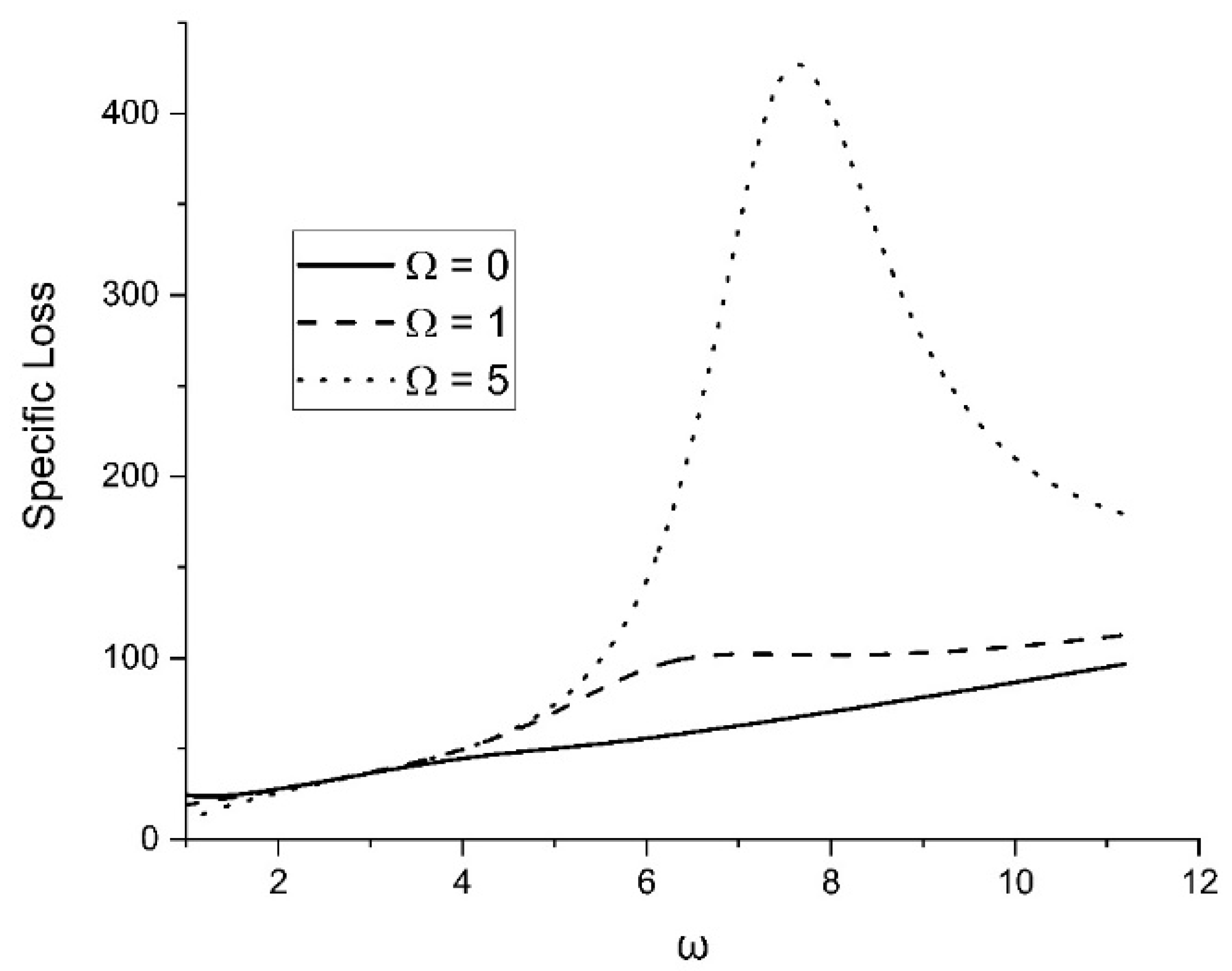
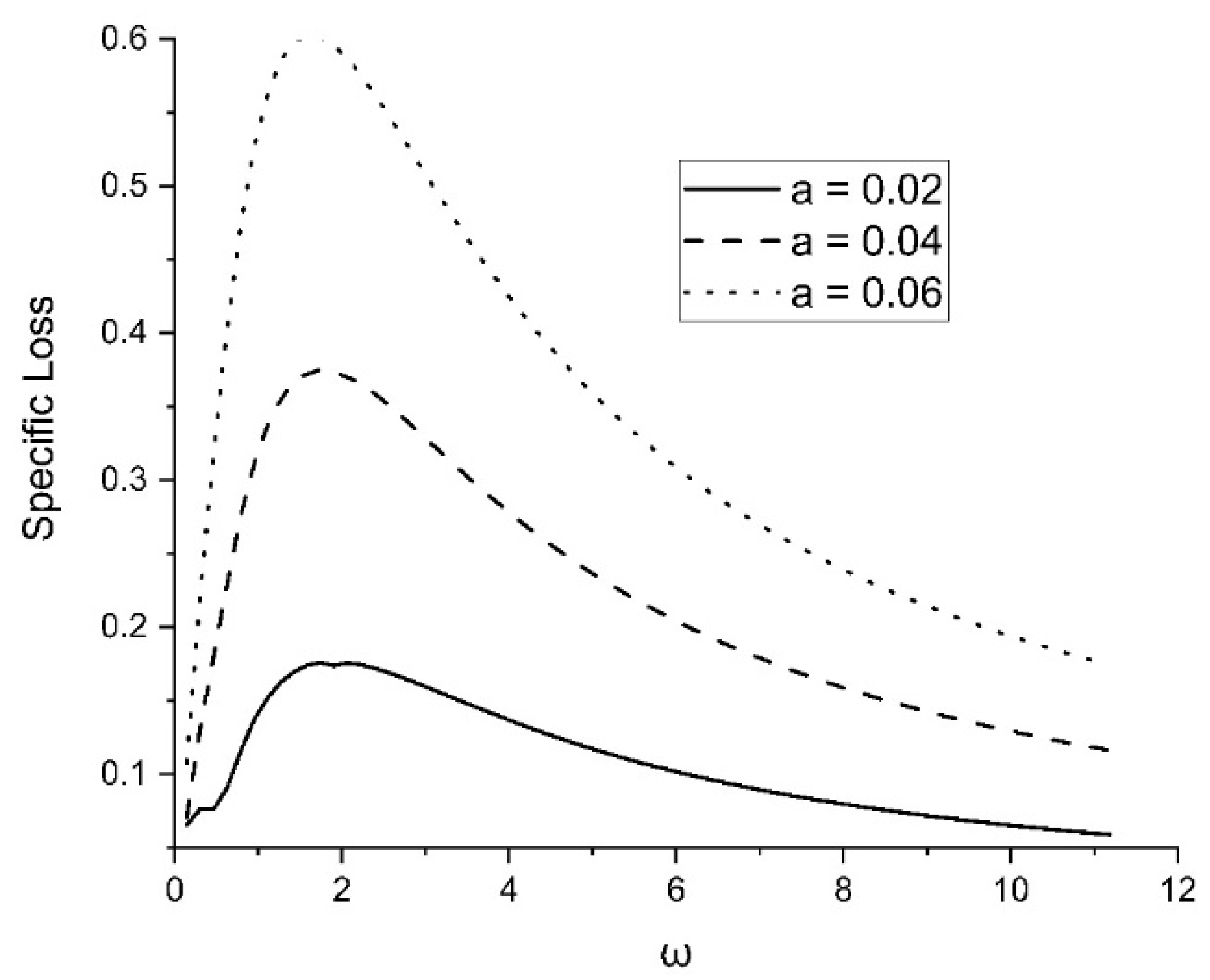
(iii) Specific Loss

The specific loss is defined as

$$W_j={\left(\frac{\mathsf{\Delta }W}{W}\right)}_j=4\pi \left|\frac{Img\left({\xi }_j\right)}{Re\left({\xi }_j\right)}\right|, j=1,2,3,4.$$

where ${ W}_1, W_2, W_3, \mathrm{a}\mathrm{n}\mathrm{d} W_4$ are the specific loss of CLD, CT, CCD, and CTD waves, respectively; $\mathsf{\Delta }W$ is the dissipated energy; and $W$ is the stored energy.

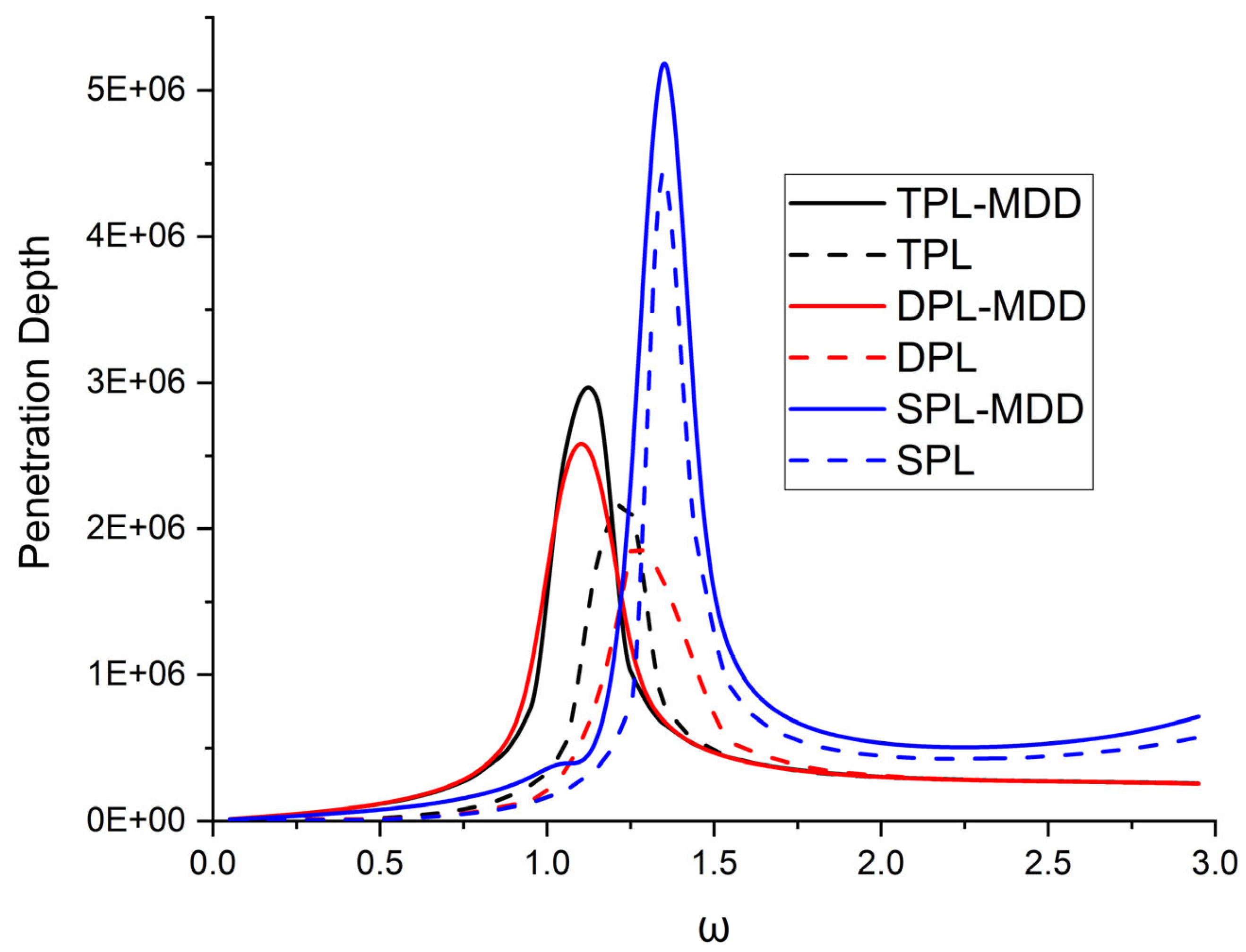
(iv) Penetration depth

We can determine the penetration depth by

$$S_j=\frac{1}{Img\left({\xi }_j\right)}, j=1,2,3,4.$$

where ${ S}_1, S_2, S_3,\mathrm{a}\mathrm{n}\mathrm{d} S_4$ represent the CLD, CT, CCD, and CTD waves’ penetration depth, respectively.

The total displacement and conductive temperature are given by

$$(\varphi ,\psi ,\phi ,N)={\sum }_{j=1}^8(1{,d}_j,l_j,m_j)A_j{e}^{i{M}_j},$$

(53)

where

$$M_0={\xi }_0\left(xsin{\theta }_0+zcos{\theta }_0\right)-\omega t,$$

$$M_j={\xi }_j\left(xsin{\theta }_j-zcos{\theta }_j\right)-\omega t, j=1,2,3,4.$$

Here, subscripts $j=0$ represent the quantities related to the incident CLD wave, whereas the subscripts $j=1, 2, 3, 4$ represent the related reflected waves, and ${\xi }_j$ are the roots of Equation (33).

$$d_j=\frac{\left({\zeta }_2+{\zeta }_4{\xi }_j^2\right)\left({\epsilon }_2{\epsilon }_3\left(1+a{\xi }_j^2\right)-\left({\zeta }_{10}+{\zeta }_{12}{\xi }_j^2\right)\left({\zeta }_9-{\xi }_j^2\right)\right)+{\zeta }_{13}{\xi }_j^2\left(\left(1+a{\xi }_j^2\right)\left({\zeta }_9-{\xi }_j^2-{\epsilon }_3\right)\right)}{\left({\zeta }_7+{\zeta }_8{\xi }_j^2\right)\left({\epsilon }_2{\epsilon }_3\left(1+a{\xi }_j^2\right)-\left({\zeta }_{10}+{\zeta }_{12}{\xi }_j^2\right)\left({\zeta }_9-{\xi }_j^2\right)\right)},$$

$$l_j=\frac{-{\zeta }_{13}{\xi }_j^2\left({\zeta }_7+{\zeta }_8{\xi }_j^2\right)+{\epsilon }_2\left(\left({\zeta }_2+{\zeta }_4{\xi }_j^2\right)\left({\zeta }_7+{\zeta }_8{\xi }_j^2\right)-\left({\zeta }_1+{\zeta }_3{\xi }_j^2\right)\left({\zeta }_5+{\zeta }_6{\xi }_j^2\right)\right)}{\left({\zeta }_7+{\zeta }_8{\xi }_j^2\right)\left({\epsilon }_2{\epsilon }_3\left(1+a{\xi }_j^2\right)-\left({\zeta }_{10}+{\zeta }_{12}{\xi }_j^2\right)\left({\zeta }_9-{\xi }_j^2\right)\right)},$$

$$m_j=\frac{\left(1+a{\xi }_j^2\right){ϵ}_1\left(\left({\zeta }_2+{\zeta }_4{\xi }_j^2\right)\left({\zeta }_7+{\zeta }_8{\xi }_j^2\right)-\left({\zeta }_1+{\zeta }_3{\xi }_j^2\right)\left({\zeta }_5+{\zeta }_6{\xi }_j^2\right)\right)}{\left({\zeta }_7+{\zeta }_8{\xi }_j^2\right)\left({\epsilon }_2{\epsilon }_3\left(1+a{\xi }_j^2\right)-\left({\zeta }_{10}+{\zeta }_{12}{\xi }_j^2\right)\left({\zeta }_9-{\xi }_j^2\right)\right)},$$

$$j=1,2,3,4.$$

The expressions of u and w can be written as

$$\begin{array}{ll}u=i{A}_0{\xi }_0(sin{\theta }_0& - d_{0}cos{\theta }_0)e^{i\left({\xi }_0\left(xsin{\theta }_0+zcos{\theta }_0\right)-\omega t\right)}\\ & +\sum _{j=1}^{4}i{A}_j{\xi }_j\left(sin{\theta }_j+d_{j}cos{\theta }_j\right)e^{i\left({\xi }_j\left(xsin{\theta }_j-zcos{\theta }_j\right)-\omega t\right)}\end{array}$$

$$\begin{array}{ll}w=i{A}_0{\xi }_0(d_{0}sin{\theta }_0& + cos{\theta }_0)e^{i\left({\xi }_0\left(xsin{\theta }_0+zcos{\theta }_0\right)-\omega t\right)}\\ & +\sum _{j=1}^{4}i{A}_j{\xi }_j\left(d_{j}sin{\theta }_j-cos{\theta }_j\right)e^{i\left({\xi }_j\left(xsin{\theta }_j-zcos{\theta }_j\right)-\omega t\right).}\end{array}$$

5. Boundary Conditions

Since the space beyond boundary z = 0 is adjacent to the vacuum, it is free from surface traction. The dimensionless, torsion-free, thermally insulated, and carrier density during a finite probability of recombination conditions at the free surface $z=0$ is

$${\sigma }_{zz}=0,$$

(54)

$${\sigma }_{xz}=0,$$

(55)

$$\frac{\partial \phi }{\partial z}=0,$$

(56)

$$D_E\frac{\partial N}{\partial z}=s_{0}N.$$

(57)

Using Equation (53) in the dimensionless boundary Equations (54)–(57) with the help of Equations (48) and (49) gives

$$\begin{array}{l}\sum _{j=1}^4{A_{j}e}^{i(-\omega t+{\xi }_j\left(xsin{\theta }_j\right))}\left[-{\xi }_j^2\left(\left(1-2{\delta }^2\right){sin}^2{\theta }_j+{cos}^2{\theta }_j\right)+{\xi }_j^2\left({\delta }^2\right)\sin 2{\theta }_j{d}_j-\left[1+a{\xi }_j^2\right]l_j-m_j\right]\\ \hspace{1em}\hspace{1em}\hspace{1em}\hspace{1em}\hspace{1em}\hspace{1em}\hspace{1em}=A_0{e}^{i\left(-\omega t+{\xi }_0\left(xsin{\theta }_0\right)\right)}[{\xi }_0^2\left(\left(1-2{\delta }^2\right){sin}^2{\theta }_0+{cos}^2{\theta }_0\right)-{\xi }_0^2\left({\delta }^2\right)\sin 2{\theta }_0{d}_0+\left[1+a{\xi }_0^2\right]l_0\\ \hspace{1em}\hspace{1em}\hspace{1em}\hspace{1em}\hspace{1em}\hspace{1em}\hspace{1em}+m_0],\end{array}$$

(58)

$$\sum _{j=1}^3{A_{j}e}^{i(-\omega t+{\xi }_j\left(xsin{\theta }_j\right))}\left[{\xi }_j^2\left(\sin 2{\theta }_j+d_j\cos {2\theta }_j\right)\right]={A_{0}e}^{i(-\omega t+{\xi }_0\left(xsin{\theta }_0\right))}\left[{\xi }_0^2\left(\left(\sin 2{\theta }_0-d_0\cos {2\theta }_0\right)\right)\right],$$

(59)

$$\sum _{j=1}^4{A_{j}e}^{i(-\omega t+{\xi }_j\left(xsin{\theta }_j\right))}\left[l_j{\xi }_{j}cos{\theta }_j\right]=A_0{e}^{i\left(-\omega t+{\xi }_0\left(xsin{\theta }_0\right)\right)}\left[l_0{\xi }_{0}cos{\theta }_0\right].$$

(60)

$$\sum _{j=1}^4{A_{j}e}^{i(-\omega t+{\xi }_j\left(xsin{\theta }_j\right))}{m}_j\left(i{\xi }_{j}cos{\theta }_j{D}_E+s_0\right)=A_0{e}^{i\left(-\omega t+{\xi }_0\left(xsin{\theta }_0\right)\right)}{m}_0\left(i{\xi }_{0}cos{\theta }_0{D}_E-s_0\right)$$

(61)

Equations (58)–(61) are satisfied $\forall \mathit{x}$; hence,

$$M_1\left(x,0\right)=M_2\left(x,0\right){=M}_3\left(x,0\right)=M_4\left(x,0\right){=M}_0\left(x,0\right).$$

(62)

From Equations (51) and (62), we obtain

$${\xi }_{1}sin{\theta }_1={\xi }_{2}sin{\theta }_2={\xi }_{3}sin{\theta }_3={\xi }_{4}sin{\theta }_4={\xi }_{0}sin{\theta }_0.$$

(63)

This is Snell’s law for the stress-free thermally insulated surface of a nonlocal rotating isotropic semiconducting thermo-magnetoelastic medium.

Equations (49)–(52) with the aid of Equations (53) and (54) yield

$${\sum }_{j=1}^4{X}_{rj}{A}_j=X_{ro}{A}_0,r=1,2,3,4.$$

(64)

where, for $j=1,2,3,4,$ we have

$$X_{1j}=\left[-{\xi }_j^2\left(\left(1-2{\delta }^2\right){sin}^2{\theta }_j+{cos}^2{\theta }_j\right)+{\xi }_j^2\left({\delta }^2\right)\sin 2{\theta }_j{d}_j-\left[1+a{\xi }_j^2\right]l_j-m_j\right],$$

(65)

$$X_{2j}=\left[{\xi }_j^2\left(\sin 2{\theta }_j+d_j\cos {2\theta }_j\right)\right],$$

(66)

$$X_{3j}=l_j{\xi }_{j}cos{\theta }_j.$$

(67)

$$X_{4j}=m_j\left(i{\xi }_{j}cos{\theta }_j{D}_E+s_0\right).$$

(68)

And we have

$$X_{10}=\left[{\xi }_0^2\left(\left(1-2{\delta }^2\right){sin}^2{\theta }_0+{cos}^2{\theta }_0\right)-{\xi }_0^2\left({\delta }^2\right)\sin 2{\theta }_0{d}_0+\left[1+a{\xi }_0^2\right]l_0+m_0\right],$$

(69)

$$X_{20}={\xi }_0^2\left(\left(\sin 2{\theta }_0-d_0\cos {2\theta }_0\right)\right),$$

(70)

$$X_{30}=\left[l_0{\xi }_{0}cos{\theta }_0\right].$$

(71)

$$X_{40}=m_0\left(i{\xi }_{0}cos{\theta }_0{D}_E-s_0\right).$$

(72)

Incident CLD Wave

If we divide the set of Equations (64) by $A_1$, then, using Cramer’s rule, we may solve a system of four equations with four unknowns as

$${ Z}_j=\frac{A_j}{A_0}=\frac{{∆}_j}{∆}, j=1,2,3,4.$$

(73)

where $Z_j(j=1,2,3,4)$ are the amplitude ratios of the reflected CLD wave, CT wave, CCD wave, and CTD wave to that of the incident CLD wave.

Here,

$$∆={\left|\begin{array}{c}\begin{array}{cc}{X}_{11}& X_{12} \\ X_{21}& X_{22} \end{array}\begin{array}{cc}{X}_{13}& X_{14}\\ X_{23}& X_{24}\end{array}\\ \begin{array}{cc}{X}_{31}& X_{32} \\ X_{41}& X_{42} \end{array}\begin{array}{cc}{X}_{33}& X_{34}\\ X_{43}& X_{44}\end{array}\end{array}\right|}_{4X4},$$

(74)

By substituting ${\left[X_{10} X_{20} X_{30} X_{40}\right]}^{\prime }$ for the first, second, and third columns ∆, one can obtain ${∆}_j \left(j=1,2,3,4\right)$.

Following Achenbach [40], “the energy flux across the surface element is represented as

$$P*={\sigma }_{lm}{n}_m{\dot{u}}_l,$$

(75)

where  $n_m$  are the direction cosines of the unit normal and  ${\dot{u}}_l$  are the components of the particle velocity.

The time average  $P*$  , over a period  $P$  denoted by  $<P*>$ is the average energy transmission per unit surface area per unit time and is given at the interface $z=0$  as

$$<P*>=<Re\left({\sigma }_{xz}\right)·Re\left(\dot{u}\right)+Re\left({\sigma }_{zz}\right)·Re\left(\dot{w}\right)>.$$

(76)

Following Achenbach [40], for complex functions $a$ and $b$, we take

$$<Re\left(a\right)><Re\left(b\right)>=\frac{1}{2}Re\left(a\overline{b}\right).$$

(77)

The expressions for energy ratios $E_j (j=1,2,3,4)$ for reflected CLD wave, CT wave, CCD wave, and CTD wave are given as

$$E_j=\frac{<P_j^{*}>}{<P_0^{*}>},j=1,2,3,4.$$

(78)

where $<P_0^{*}>$ is corresponding to the incident CLD wave, and $<P_j^{*}>, j=1, 2, 3, 4$ represents average energies transmission per unit surface area per unit time, resulting in reflected CLD wave, CT wave, CCD wave, and CTD wave, respectively.

$$\begin{array}{ll}{P}_j^{*}=\frac{1}{2}Re\{A_j^2{\xi }_j^2\omega & \{-\left(\sin 2{\theta }_j-d_j\cos 2{\theta }_j\right)\left(\sin {\theta }_j+d_j\cos {\theta }_j\right){\xi }_j^2{\delta }^2\\ & +\left[-{\xi }_j^2\left(\left(1-2{\delta }^2\right){sin}^2{\theta }_j+{cos}^2{\theta }_j\right)-{\xi }_j^2\left({\delta }^2\right)\sin 2{\theta }_j{d}_j-\left[1+a{\xi }_j^2\right]l_j-m_j\right](d_{j}sin{\theta }_j\\ & -cos{\theta }_j\left)\right\}\},j=\mathrm{0,1},\mathrm{2,3},4.\end{array}$$

The conservation of energy states that the total energy always remains conserved, mathematically expressed as follows:

$$E_1+E_2+E_3+E_4=1.$$

6. Particular Cases

• For a nonlocal semiconductor medium with two temperatures, rotation, and Hall current $\left(m,a,\mathsf{\Omega },\xi \right)>0$, the following cases can also be achieved:

  i.

  If we consider ${\tau }_q>{\tau }_T>{\tau }_v\ge 0$ in the above relationships, three-phase lag with MDD (TPL-MDD) can be obtained.

  ii.

  If we consider ${\tau }_v=0,K_{ij}^{\mathrm{*}}=0{\tau }_q>{\tau }_T\ge 0,$ dual-phase lag MDD (DPL-MDD) can be achieved.

  iii.

  If ${\tau }_T=0,{\tau }_v=0,{\tau }_q={\tau }_0>0$ and $K_{ij}^{\mathrm{*}}=0$, and ignoring ${\tau }_q^2,$ Lord–Shulman MDD or single-phase lag MDD (SPL-MDD) can be achieved.

  iv.

  If we take ${\tau }_q>{\tau }_T>{\tau }_v\ge 0,\text{and} \text{take} G_{{\tau }_q}=G_{{\tau }_v}=G_{{\tau }_T}=i\omega$, three-phase lag without MDD (TPL) can be retrieved.

  v.

  By taking ${\tau }_v=0,K_{ij}^{\mathrm{*}}=0,$ and ${\tau }_q>{\tau }_T\ge 0,\text{and} \text{taking} G_{{\tau }_q}=G_{{\tau }_T}=i\omega ,$ DPL can be found.

  vi.

  Moreover, by considering ${\tau }_T=0,{\tau }_v=0,{\tau }_q={\tau }_0>0$ and $K_{ij}^{\mathrm{*}}=0$, ignoring ${\tau }_q^2$, and taking $G_{{\tau }_q}=i\omega ,$ we found the Lord–Shulman model or single-phase lag (SPL).

  vii.

  In addition, GN-III theory can be obtained by taking ${\tau }_T=0,{\tau }_v=0,{\tau }_q=0$ and $K_{ij}^{\mathrm{*}}\ne 0,K_{ij}\ne 0$.

  viii.

  Also, if we consider ${\tau }_T=0,{\tau }_v=0,{\tau }_q=0$ and $K_{ij}=0,$ it results in GN-II.

  ix.

  ${\tau }_T=0,{\tau }_v=0,{\tau }_q=0$

• If we consider $ϵ=0$, for case 1(a–i), it results in a local semiconductor medium.
• By taking $\mathsf{\Omega }=0$, for case 1(a–i), the results are without rotation.
• By taking $\mathrm{m}=0$, for case 1(a–i), the results are without Hall current.
• If we take $a_1=0$, for case 1(a–i), the results are without two temperatures.

7. Numerical Results and Discussion

To validate the theoretical results with Hall current, different theories of thermoelasticity, and two temperatures, the physical data for silicon material are taken from Mahdy et al. [37] as

$$\begin{array}{ll}\lambda =3.64\times {10}^{10} {\mathrm{Nm}}^{-2},& \mu =5.46\times {10}^{10} {\mathrm{Nm}}^{-2}, \beta =7.04\times {10}^6 {\mathrm{Nm}}^{-2}{\mathrm{deg}}^{-1}, { d}_n\\ & =-9\times {10}^{-31} {\mathrm{m}}^{-3}, \rho =2.33\times {10}^3 {\mathrm{Kgm}}^{-3}, C_E\\ & =695 {\mathrm{JKg}}^{-1}{\mathrm{K}}^{-1}, K=150 {\mathrm{Wm}}^{-1}{\mathrm{K}}^{-1}, K*\\ & =1.54\times {10}^2 \mathrm{Ws}, {\mathrm{T}}_0=800 \mathrm{K},{\tau }_T=1\times {10}^{-7}{\tau }_v\\ & =2\times {10}^{-8} \mathrm{s}, {\tau }_q=2\times {10}^{-7} \mathrm{s},D_E=2.5\times {10}^{-3} {\mathrm{m}}^2{\mathrm{s}}^{-1},{\mathrm{H}}_0\\ & =1 \mathrm{J}{\mathrm{m}}^{-1}\mathrm{n}{\mathrm{b}}^{-1},\mathsf{\tau }=5\times {10}^{-5} \mathrm{s}, N_0={10}^{20} {\mathrm{m}}^{-3}, s_0\\ & =2 {\mathrm{ms}}^{-1}, {\mathsf{\epsilon }}_0=8.838\times {10}^{-12} \mathrm{F}{\mathrm{m}}^{-1},E_g=1.11 \mathrm{eV}, {\alpha }_T\\ & =3\times {10}^{-6} {\mathrm{K}}^{-1}.\end{array}$$

The nonsingular kernel function $K(t-\eta )$ used here is

$$K\left(t-\eta \right)={\left[1+\left(\eta -t\right)/\omega \right]}^2$$

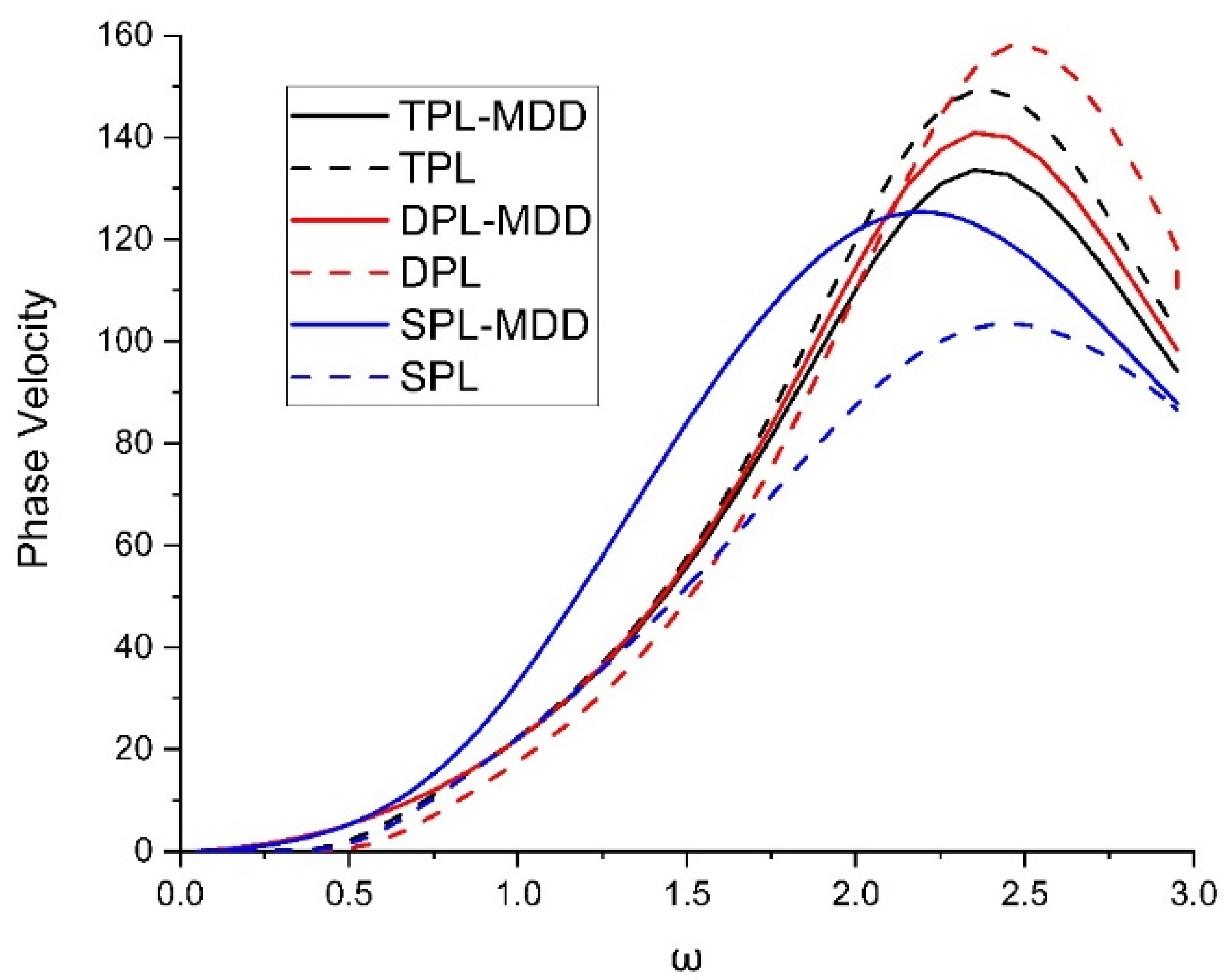
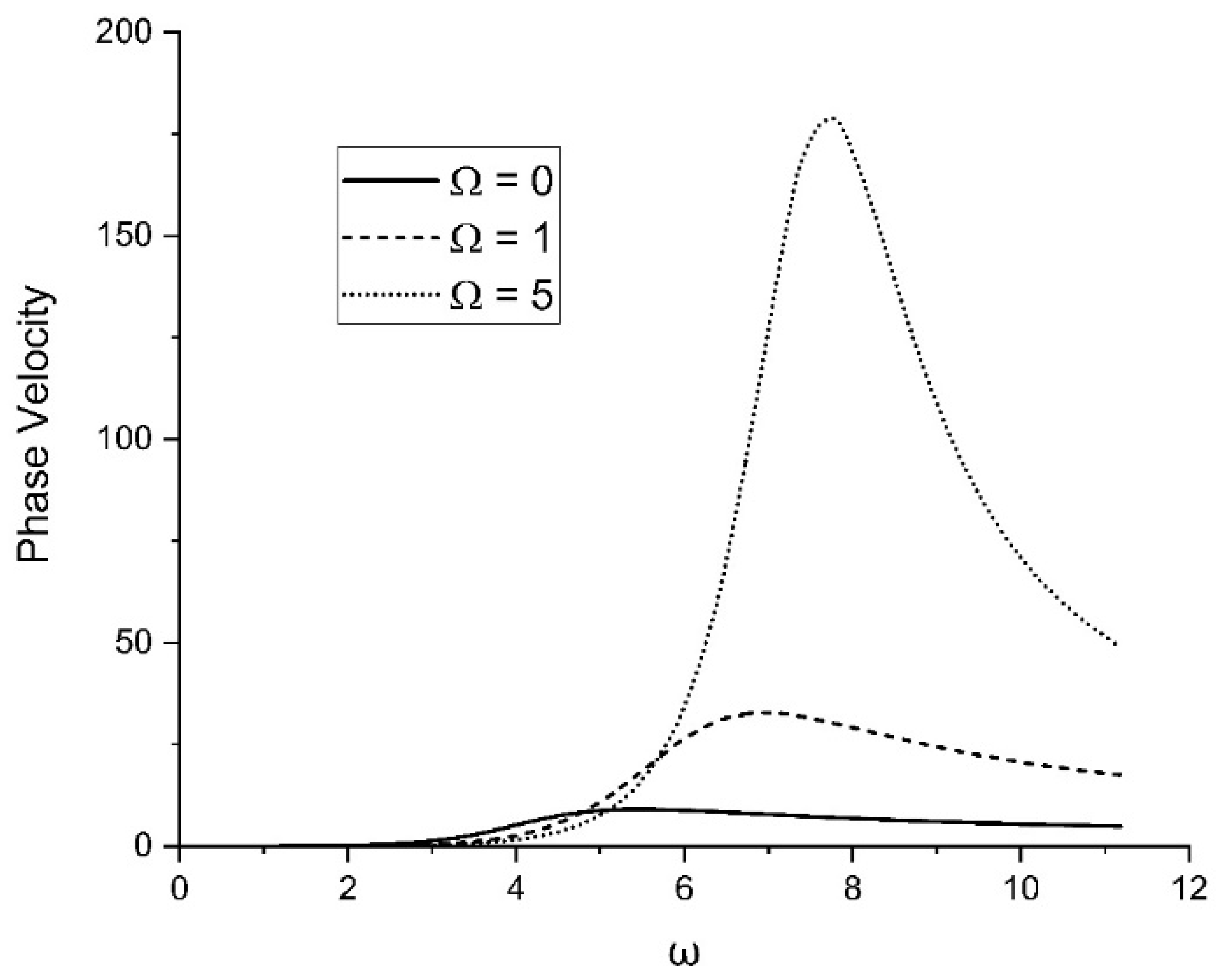
Figure 2 demonstrates the variation in phase velocity with the different theories of thermoelasticity (TPL-MDD, TPL, DPL-MDD, DPL, SPL-MDD, and SPL). Different theories show the different impacts on the phase velocity of a plane wave in a semiconducting material. Figure 3 demonstrates the variation in phase velocity with respect to variation in the rotation parameter $\mathsf{\Omega }.$ As the rotation parameter $\mathsf{\Omega }$ increases, phase velocity also increases. 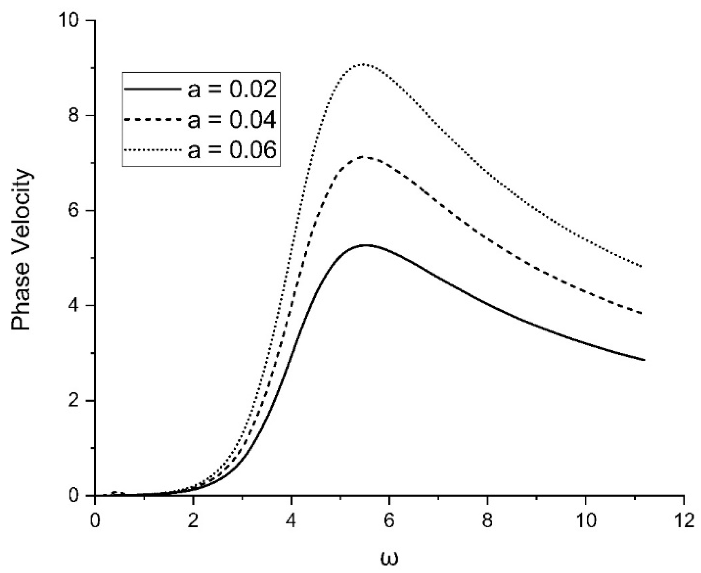Figure 4 shows the variation in phase velocity with respect to the variation in the two-temperature parameter $a.$ The phase velocity of the plane wave decreases with increasing values of the two temperatures.

Figure 5 demonstrates the variation in attenuation coefficients with the different theories of thermoelasticity (TPL-MDD, TPL, DPL-MDD, DPL, SPL-MDD, and SPL). Different theories show the different impacts on the attenuation coefficients of a plane wave in a semiconducting material. Figure 6 demonstrates the variation in attenuation coefficients with the variation in rotation parameter $\mathsf{\Omega }.$ Attenuation coefficients rapidly fall for the frequency’s initial value. However, attenuation coefficients likewise rise with the rotation parameter. Figure 7 shows how the two-temperature parameters modify the attenuation coefficients. The attenuation coefficients of a planar wave decrease as the two temperatures increase.

Figure 8 illustrates the variation in specific loss with the different theories of thermoelasticity (TPL-MDD, TPL, DPL-MDD, DPL, SPL-MDD, and SPL). Different theories demonstrate the various effects on a semiconducting material’s specific loss of plane waves. Figure 9 shows how the rotation parameter’s effect on specific loss can be changed. Specific loss increases with an increase in the rotation parameter. Figure 10 shows how the two-temperature parameters change the specific loss. The specific loss of a plane wave increases with the value of the two temperatures.

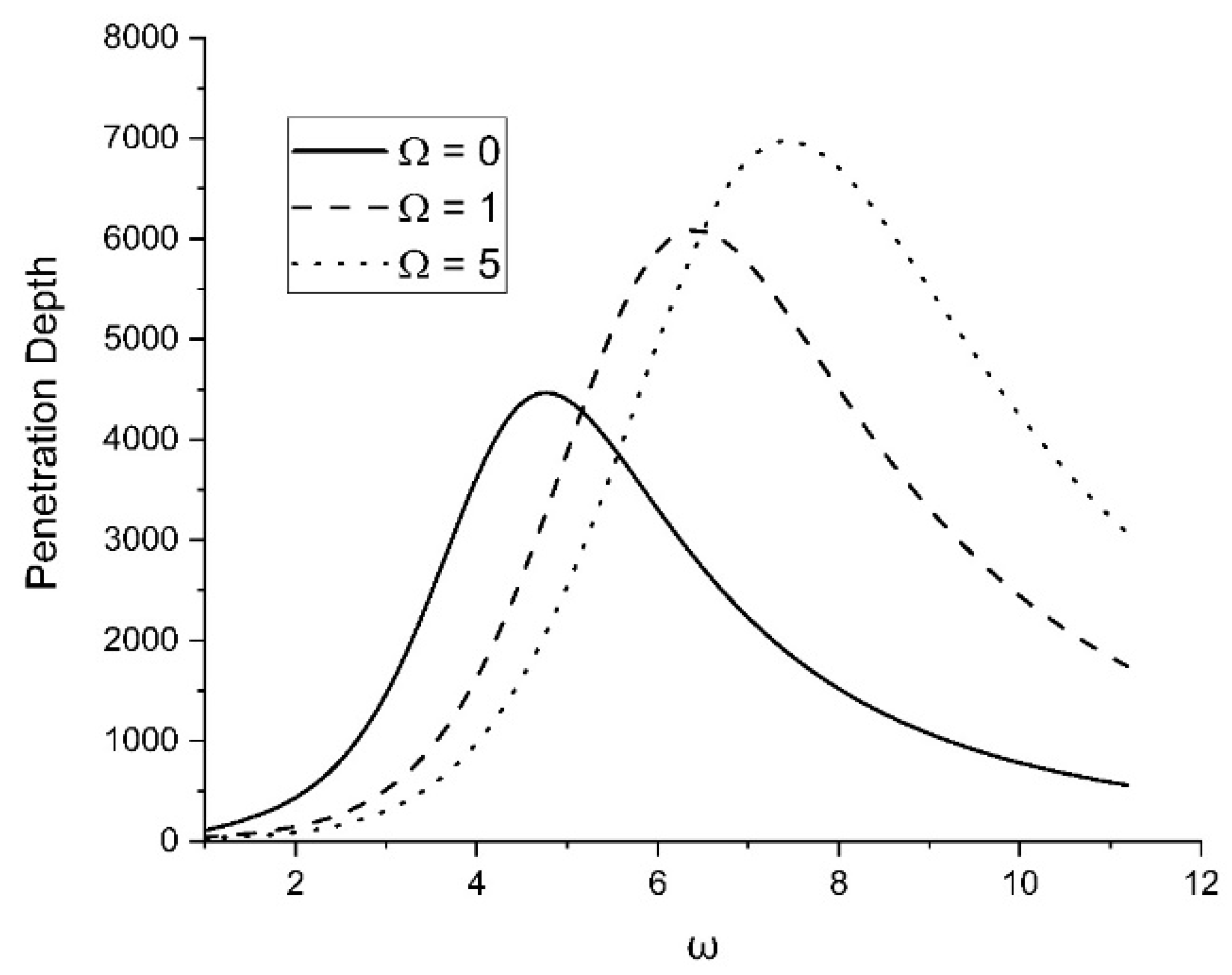
Figure 11 illustrates the variation in penetration depth for the different theories of thermoelasticity (TPL-MDD, TPL, DPL-MDD, DPL, SPL-MDD, and SPL). Diverse theories demonstrate the various effects on the depth to which plane waves can penetrate a semiconducting material. Figure 12 illustrates the change in penetration depth with respect to the rotation parameter $\mathsf{\Omega }.$ The penetration depth rises substantially for the early values of the frequency and falls after the first half of the frequency range. The penetration depth, however, increases with the value of the rotational parameter. 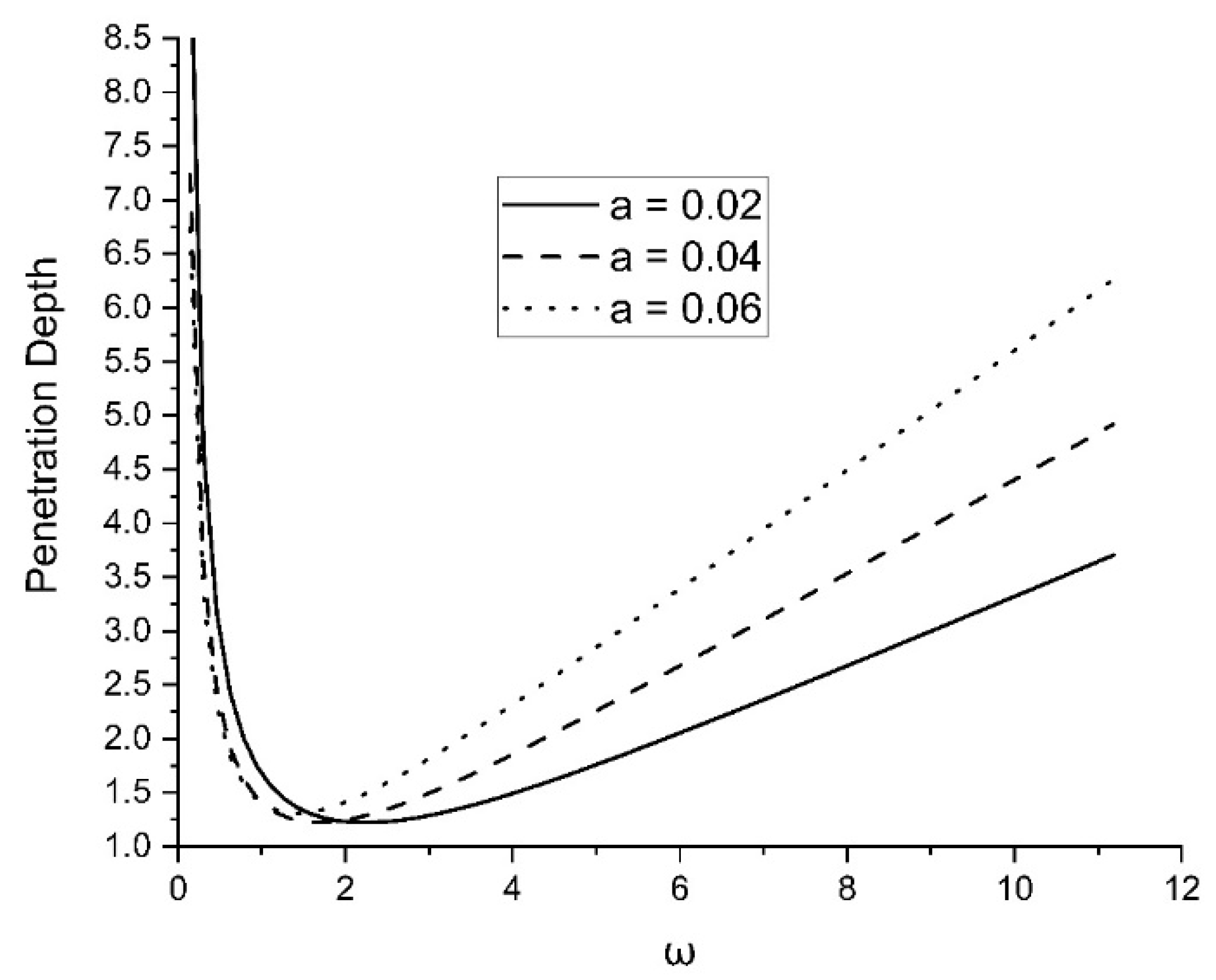Figure 13 demonstrates the variation in the penetration depth with the variation in $a.$ The penetrating depth of the plane wave increases as the two temperatures increase.

8. Conclusions

• We examined the reflection of a plane wave in a stress-free, thermally insulated, and diffusion-transported semiconducting magneto-thermoelastic rotating nonlocal half-space medium. A novel mathematical model for extended three-phase-lag (TPL) heat transfer with two temperatures (2T) and memory-dependent derivative (MDD) was developed for this problem.
• Under a strong magnetic field, the semiconducting medium is rotating with angular frequency $\Omega$ The governing equations are expressed with the help of the Hall current, TPL MDD heat transfer, and 2T.
• The dimensionless expressions for an attenuation coefficient, penetration depth, phase velocity, specific loss, and energy ratios and amplitude ratios of different reflected waves were obtained.
• Graphs were used to illustrate the effect of different theories such as TPL-MDD, TPL, DPL-MDD, DPL, and SPL-MDD and SPL, rotation, and two temperatures on the phase velocities, specific loss, penetration depth, and attenuation coefficients of different reflected waves. The results showed that different theories, such as TPL-MDD, TPL, DPL-MDD, DPL, SPL-MDD, and SPL, produce different variations in the characteristics of the plane wave. The penetration depth, attenuation coefficients, specific loss, and phase velocities of the plane wave also increase as the value of rotation increases. The variances in the different plane wave characteristics likewise increase when the two-temperature parameters rise.
• The change in the kernel function’s values causes the waves to disperse based on the wave velocity equation. Additionally, different special cases were considered while formulating the problem and calculating the numerical results.
• The findings could be useful for the fabrication of semiconductor nanostructure devices like MEMS/NEMS, magnetic switches, and Hall effect sensors, as well as for seismology, geology, and automotive applications.

References

- Sherief, H.H.; El-Sayed, A.; El-Latief, A.A. Fractional order theory of thermoelasticity. Int. J. Solids Struct. 2010, 47, 269–275. [Google Scholar] [CrossRef]
- Povstenko, Y.Z. Fractional heat conduction equation and associated thermal stress. J. Therm. Stress. 2004, 28, 83–102. [Google Scholar] [CrossRef]
- Youssef, H.M. Theory of generalized thermoelasticity with fractional order strain. J. Vib. Control 2016, 22, 3840–3857. [Google Scholar] [CrossRef]
- Ezzat, M.A.; El-Karamany, A.S.; Ezzat, S.M. Two-temperature theory in magneto-thermoelasticity with fractional order dual-phase-lag heat transfer. Nucl. Eng. Des. 2012, 252, 267–277. [Google Scholar] [CrossRef]
- Youssef, H.M.; Abbas, I.A. Fractional order generalized thermoelasticity with variable thermal conductivity. J. Vibroengineering 2014, 16, 4077–4087. [Google Scholar]
- Duhamel, J.M. Memories of the molecular actions developed by changes in temperatures in solids. Mummy Div. Sav. Acad. Sci. Par. 1938, 5, 440–498. [Google Scholar]
- Catteno, C. A form of heat conduction equation which eliminates the paradox ofinstantaneous propagation. Comput. Rendus 1958, 247, 431–433. [Google Scholar]
- Vernotte, P. Some possible complications in the phenomena of thermal conduction. Comptes Rendus Acad. Sci. Paris Ser. II 1961, 252, 2190–2191. [Google Scholar]
- Green, A.E.; Naghdi, P.M. A re-examination of the basic postulates of thermomechanics. Proc. R. Soc. Lond. Ser. A Math. Phys. Sci. 1991, 432, 171–194. [Google Scholar] [CrossRef]
- Green, A.E.; Naghdi, P.M. On undamped heat waves in an elastic solid. J. Therm. Stress. 1992, 15, 253–264. [Google Scholar] [CrossRef]
- Green, A.E.; Naghdi, P.M. Thermoelasticity without energy dissipation. J. Elast. 1993, 31, 189–208. [Google Scholar] [CrossRef]
- Tzou, D.Y. A Unified Field Approach for Heat Conduction from Macro- to Micro-Scales. J. Heat Transf. 1995, 117, 8–16. [Google Scholar] [CrossRef]
- Tzou, D.Y. Experimental support for the lagging behavior in heat propagation. J. Thermophys. Heat Transf. 1995, 9, 686–693. [Google Scholar] [CrossRef]
- Yu, Y.-J.; Hu, W.; Tian, X.-G. A novel generalized thermoelasticity model based on memory-dependent derivative. Int. J. Eng. Sci. 2014, 81, 123–134. [Google Scholar] [CrossRef]
- Ezzat, M.A.; El-Karamany, A.S.; El-Bary, A.A. Generalized thermoelasticity with memory-dependent derivatives involving two temperatures. Mech. Adv. Mater. Struct. 2016, 23, 545–553. [Google Scholar] [CrossRef]
- Wang, J.-L.; Li, H.-F. Surpassing the fractional derivative: Concept of the memory-dependent derivative. Comput. Math. Appl. 2011, 62, 1562–1567. [Google Scholar] [CrossRef]
- Eringen, A.C. On differential equations of nonlocal elasticity and solutions of screw dislocation and surface waves. J. Appl. Phys. 1983, 54, 4703–4710. [Google Scholar] [CrossRef]
- Lam, D.C.C.; Yang, F.; Chong, A.; Wang, J.; Tong, P. Experiments and theory in strain gradient elasticity. J. Mech. Phys. Solids 2003, 51, 1477–1508. [Google Scholar] [CrossRef]
- Tang, F.; Song, Y. Wave reflection in semiconductor nanostructures. Theor. Appl. Mech. Lett. 2018, 8, 160–163. [Google Scholar] [CrossRef]
- Alshaikh, F. Mathematical modeling of photothermal wave propagation in a semiconducting medium due to L-S theory with diffusion and rotation effects. Mech. Based Des. Struct. Mach. 2020, 50, 2301–2316. [Google Scholar] [CrossRef]
- Kaur, I.; Lata, P.; Singh, K. Reflection of plane harmonic wave in rotating media with fractional order heat transfer. Adv. Mater. Res. 2020, 9, 289–309. [Google Scholar] [CrossRef]
- Lata, P.; Kaur, I.; Singh, K. Reflection of Plane Harmonic Wave in Transversely Isotropic Magneto-thermoelastic with Two Temperature, Rotation and Multi-dual-Phase Lag Heat Transfer. In Mobile Radio Communications and 5G Networks: Proceedings of MRCN 2020; Springer: Singapore, 2021; pp. 521–551. [Google Scholar] [CrossRef]
- Jahangir, A.; Tanvir, F.; Zenkour, A.M. Photo-thermo-elastic interaction in a semiconductor material with two relaxation times by a focused laser beam. Adv. Aircr. Spacecr. Sci. 2020, 7, 41–52. [Google Scholar]
- Othman, M.I.; Lotfy, K. Two-Dimensional Problem of Generalized Magneto-Thermoelasticity with Temperature Dependent Elastic Moduli for Different Theories. Multidiscip. Model. Mater. Struct. 2009, 5, 235–242. [Google Scholar] [CrossRef]
- Lata, P.; Kaur, I. Plane wave propagation in transversely isotropic magneto-thermoelastic rotating medium with fractional order generalized heat transfer. Struct. Monit. Maint. 2019, 6, 191–218. [Google Scholar] [CrossRef]
- Taye, I.M.; Lotfy, K.; El-Bary, A.A.; Alebraheem, J.; Asad, S. The Hyperbolic Two Temperature Semiconducting Thermoelastic Waves by Laser Pulses. Comput. Mater. Contin. 2021, 67, 3601–3618. [Google Scholar] [CrossRef]
- Marin, M.; Öchsner, A. The effect of a dipolar structure on the Hölder stability in Green–Naghdi thermoelasticity. Contin. Mech. Thermodyn. 2017, 29, 1365–1374. [Google Scholar] [CrossRef]
- Saeed, T.; Abbas, I.; Marin, M. A GL Model on Thermo-Elastic Interaction in a Poroelastic Material Using Finite Element Method. Symmetry 2020, 12, 488. [Google Scholar] [CrossRef]
- Kiani, K.; Gharebaghi, S.A.; Mehri, B. In-plane and out-of-plane waves in nanoplates immersed in bidirectional magnetic fields. Struct. Eng. Mech. 2017, 61, 65–76. [Google Scholar] [CrossRef]
- Lotfy, K.; Seddeek, M.A.; Hassanin, W.S.; El-Dali, A. Analytical Solutions of Photo-Generated Moore–Gibson–Thompson Model with Stability in Thermoelastic Semiconductor Excited Material. Silicon 2022, 14, 12447–12457. [Google Scholar] [CrossRef]
- Hashmat, A.; Adnan, J.; Aftab, K. Reflection of thermo-elastic wave in semiconductor nanostructures nonlocal porous medium. J. Central South Univ. 2020, 27, 3188–3201. [Google Scholar] [CrossRef]
- Singh, B.; Bijarnia, R. Nonlocal effects on propagation of waves in a generalized thermoelastic solid half space. Struct. Eng. Mech. 2021, 77, 473–479. [Google Scholar] [CrossRef]
- Lotfy, K.; Tantawi, R.S. Photo-Thermal-Elastic Interaction in a Functionally Graded Material (FGM) and Magnetic Field. Silicon 2020, 12, 295–303. [Google Scholar] [CrossRef]
- Ezzat, M.A.; El-Karamany, A.S.; El-Bary, A.A. A novel magneto-thermoelasticity theory with memory-dependent derivative. J. Electromagn. Waves Appl. 2015, 29, 1018–1031. [Google Scholar] [CrossRef]
- Ezzat, M.A.; El Karamany, A.S.; El-Bary, A. Thermoelectric viscoelastic materials with memory-dependent derivative. Smart Struct. Syst. 2017, 19, 539–551. [Google Scholar] [CrossRef]
- Kaur, I.; Lata, P.; Singh, K. Reflection and refraction of plane wave in piezo-thermoelastic diffusive half spaces with three phase lag memory dependent derivative and two-temperature. Waves Random Complex Media 2020, 32, 2499–2532. [Google Scholar] [CrossRef]
- Mahdy, A.M.S.; Lotfy, K.; Ahmed, M.H.; El-Bary, A.; Ismail, E.A. Electromagnetic Hall current effect and fractional heat order for microtemperature photo-excited semiconductor medium with laser pulses. Results Phys. 2020, 17, 103161. [Google Scholar] [CrossRef]
- Othman, M.I.A.; Abd-Elaziz, E.M. Effect of initial stress and Hall current on a magneto-thermoelastic porous medium with microtemperatures. Indian J. Phys. 2019, 93, 475–485. [Google Scholar] [CrossRef]
- Cemal Eringen, A. Nonlocal Continuum Field Theories; Springer: New York, NY, USA, 2004. [Google Scholar] [CrossRef]
- Achenbach, J.D. Wave Propagation in Elastic Solids; Elsevier: Amsterdam, The Netherlands, 1973. [Google Scholar]