
Target-Network Update Linked with Learning Rate Decay Based on Mutual Information and Reward in Deep Reinforcement Learning


Abstract
:1. Introduction
2. Related Works
2.1. Studies of Deep Neural Networks Using Mutual Information
2.2. Deep Reinforcement Learning with Target-Network Update
3. Proposed Algorithm
| Algorithm 1: Algorithm DQN Combined with Mutual Information and the Reward for Target-Network Update and Learning Rate |
| Initialize replay memory to capacity Initialize the main action-value with Initialize the target action-value with Initialize for and Initialize R by theoretical MI upper bound of the reward of the emulation Initialize between and and by system designers Initialize = and = 1.0 for e = 1, M do Initialize sequence = and = for t = 1, T do With probability ε, select a random action Otherwise, select Execute action and observe reward and sequence Set = and = Store transition (, , , ) in Sample random mini-batch of transitions (, , , ) from Compute = #how far from the value it achieves Compute = #MI between mini-batch If < ϵ then, Set to Set Update-Target to TRUE Set = if it terminates at step j + 1 Set = + otherwise Perform a gradient descent step on ( − with respect to θ If Update-Target is True then, Set = Set Update-Target to False End for End for |
4. Results
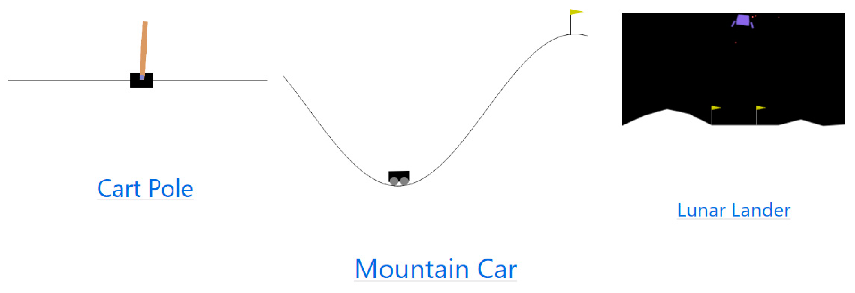
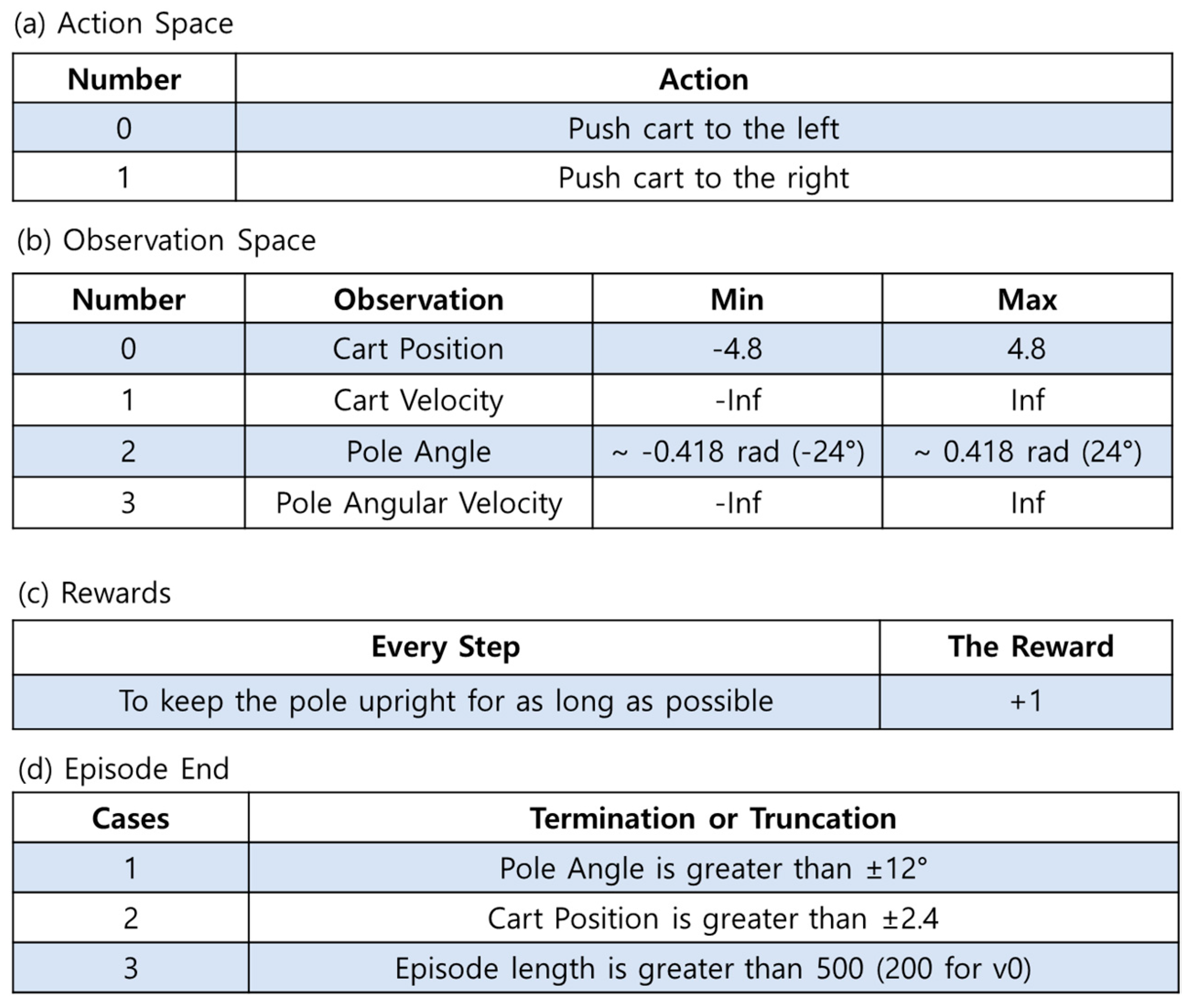
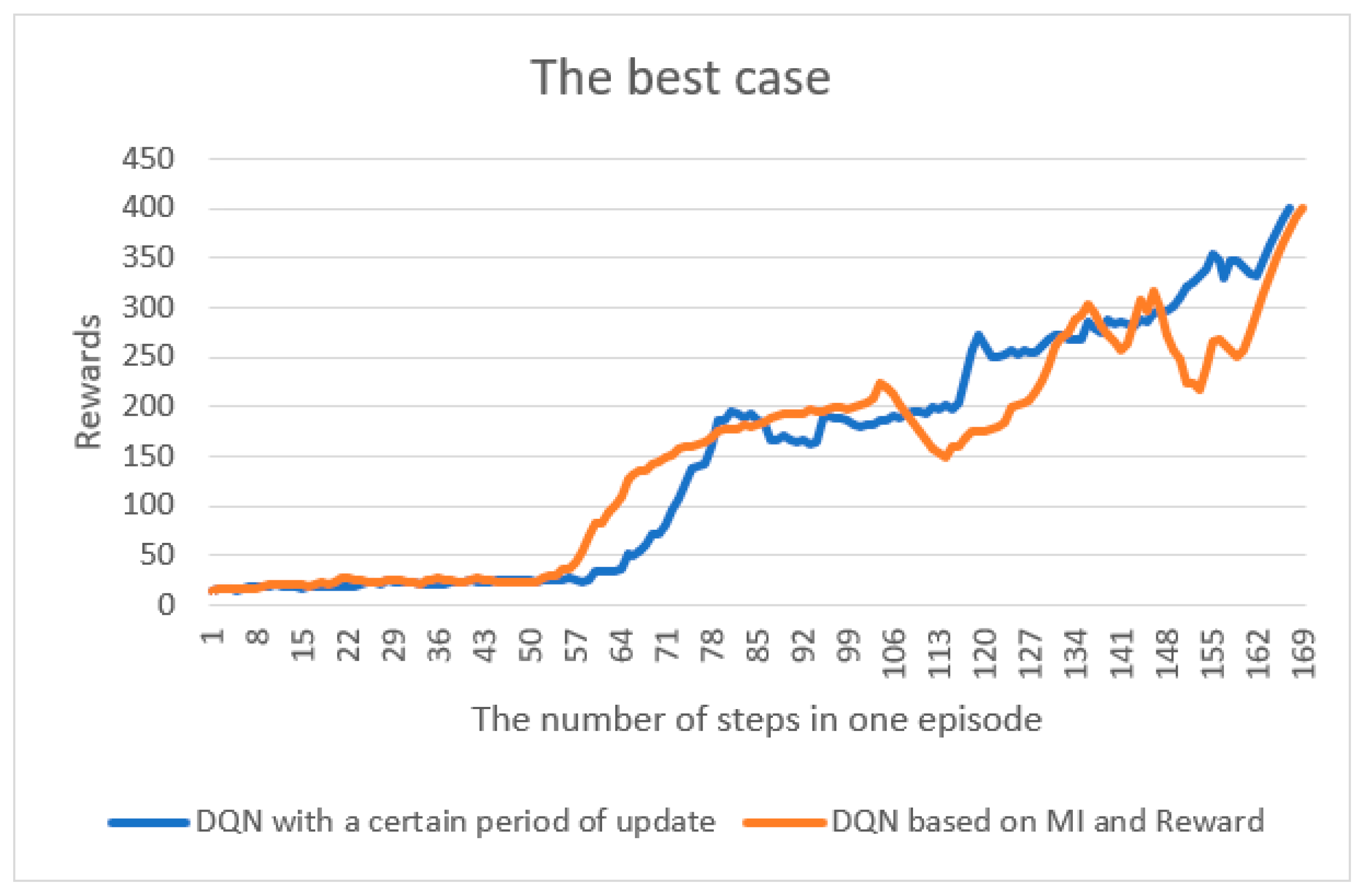
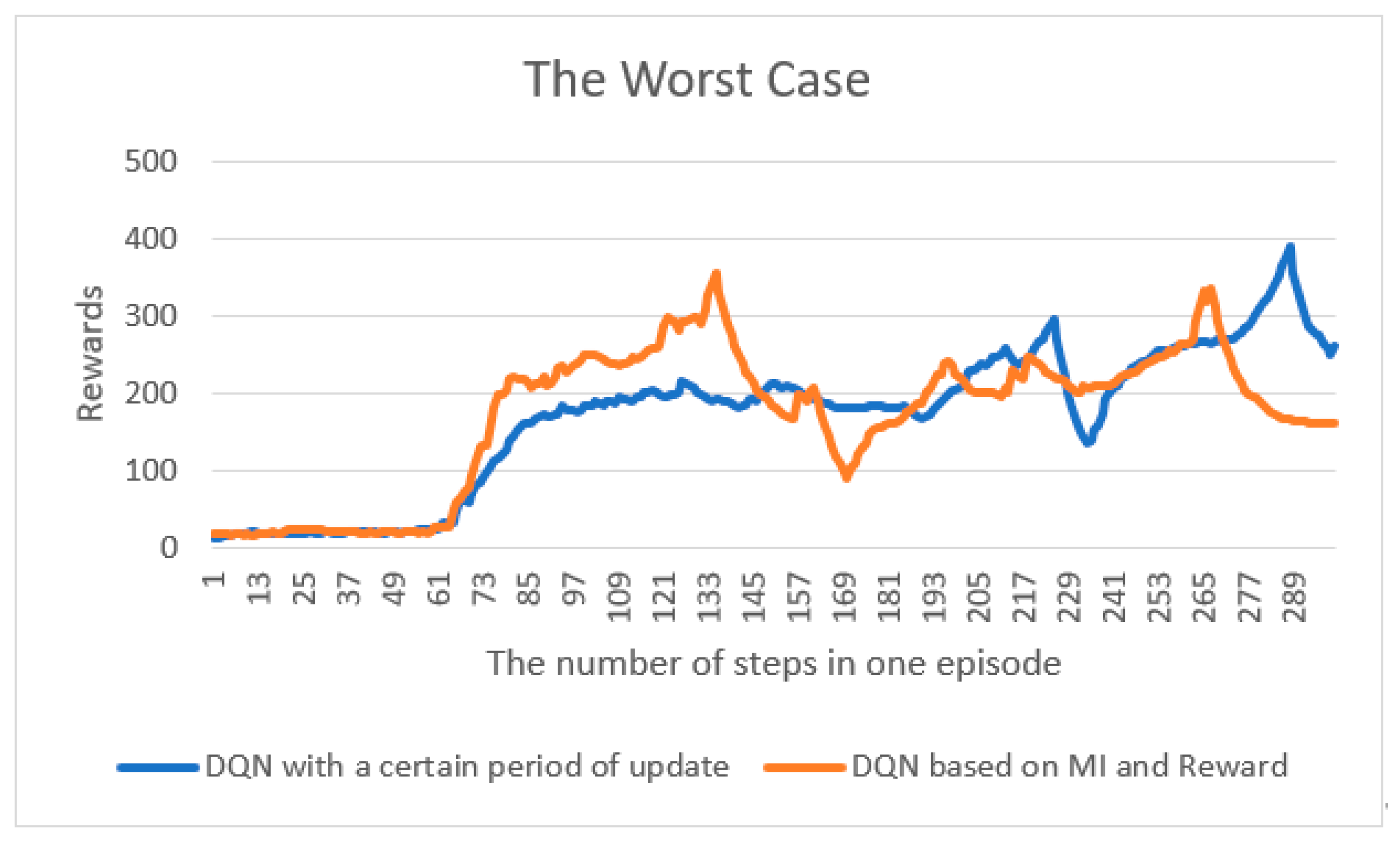
4.1. Cart-Pole
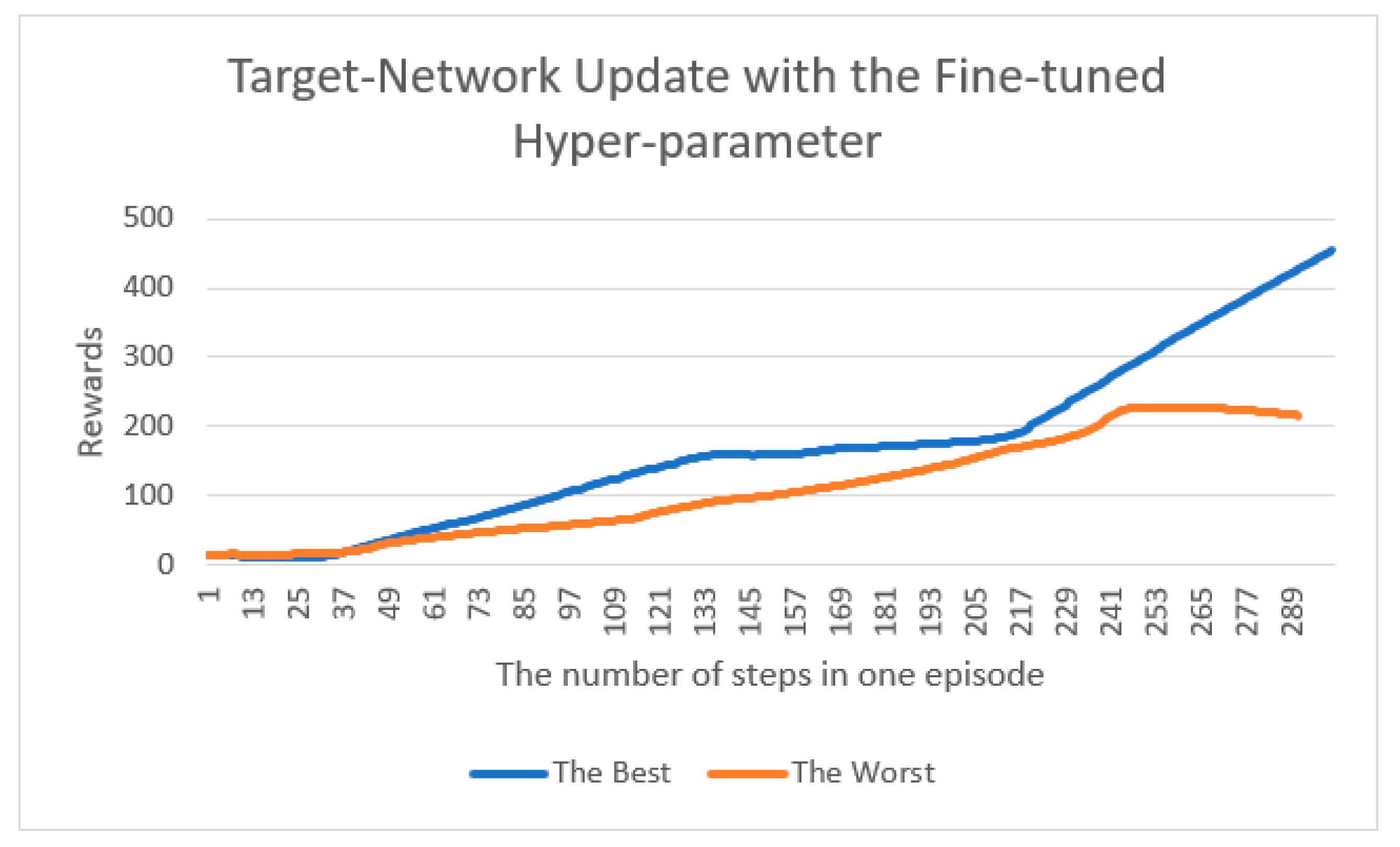
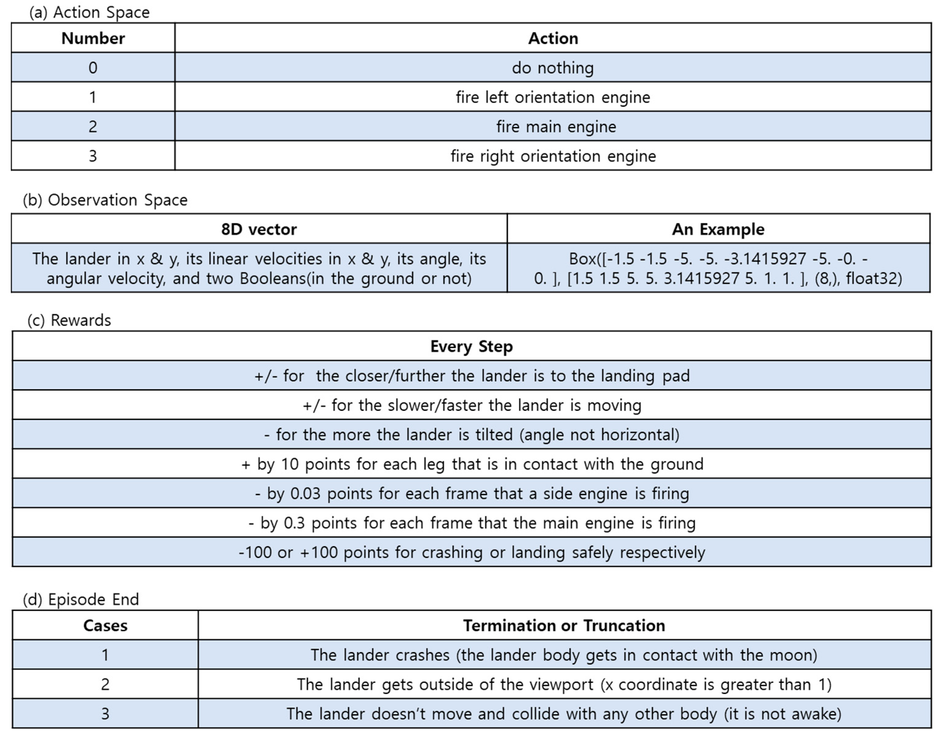
4.2. LunarLander
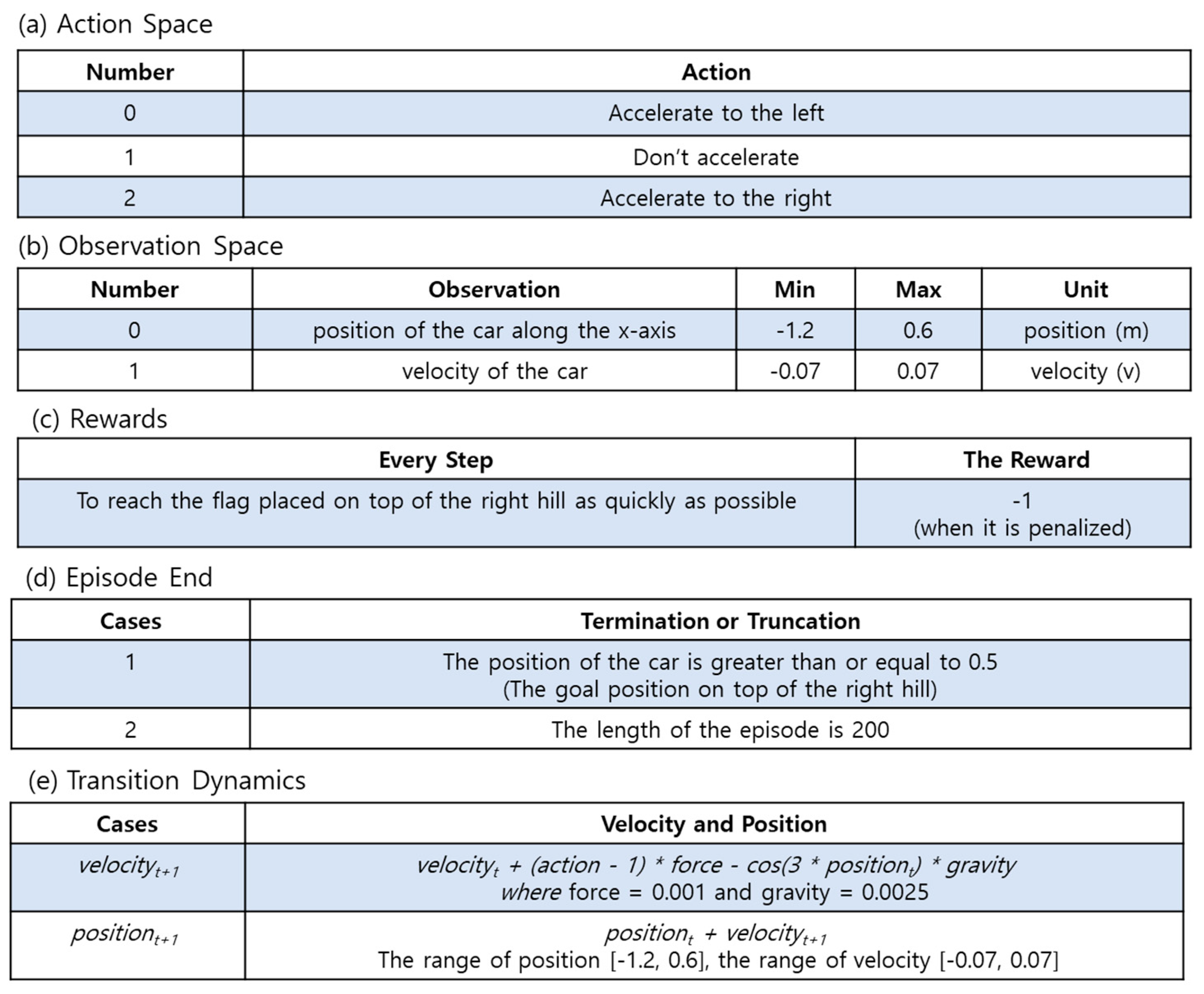
4.3. MountainCar
5. Conclusions
Funding
Data Availability Statement
Conflicts of Interest
References
- Krizhevsky, A.; Sutskever, I.; Hinton, G.E. Imagenet classification with deep convolutional neural networks. In Proceedings of the 25th International Conference on Neural Information Processing Systems, Lake Tahoe, NV, USA, 3–6 December 2012; pp. 1097–1105. [Google Scholar]
- Naderpour, H.; Mirrashid, M. Bio-inspired predictive models for shear strength of reinforced concrete beams having steel stirrups. Soft Comput. 2020, 24, 12587–12597. [Google Scholar] [CrossRef]
- Pang, X.; Zhou, Y.; Wang, P.; Lin, W.; Chang, V. An innovative neural network approach for stock market prediction. J. Supercomput. 2020, 76, 2098–2118. [Google Scholar] [CrossRef]
- Sutton, R.S.; Barto, A.G. Reinforcement Learning: An Introduction, 2nd ed.; MIT Press: Cambridge, MA, USA, 2018. [Google Scholar]
- Mnih, V.; Kavukcuoglu, K.; Silver, D.; Rusu, A.; Veness, J.; Bellemare, M.; Graves, A.; Riedmiller, M.; Fidjeland, A.; Ostrovski, G.; et al. Human-level control through deep reinforcement learning. Nature 2015, 518, 529–533. [Google Scholar] [CrossRef] [PubMed]
- Andrychowicz, M.; Wolski, F.; Ray, A.; Schneider, J.; Fong, R.; Welinder, P.; McGrew, B.; Tobin, J.; Abbeel, O.P.; Zaremba, W. Hindsight experience replay. In Proceedings of the 31st Conference on Neural Information Processing Systems (NIPS 2017), Long Beach, CA, USA, 4–9 December 2017; pp. 5048–5058. [Google Scholar]
- Osband, I.; Blundell, C.; Pritzel, A.; Van Roy, B. Deep exploration via bootstrapped DQN. In Proceedings of the 30th Conference on Neural Information Processing System (NIPS 2016), Barcelona, Spain, 5–10 December 2016; pp. 4026–4034. [Google Scholar]
- Schulman, J.; Wolski, F.; Dhariwal, P.; Radford, A.; Klimov, O. Proximal policy optimization algorithms. arXiv 2017, arXiv:1707.06347. [Google Scholar]
- Van Hasselt, H.; Guez, A.; Silver, D. Deep Reinforcement Learning with Double Q-learning. In Proceedings of the AAAI’16 Thirtieth AAAI Conference on Artificial Intelligence, Phoenix, AZ USA, 12–17 February 2016; pp. 2094–2100. [Google Scholar]
- Stooke, A.; Abbeel, P. rlpyt: A research code base for deep reinforcement learning in pytorch. arXiv 2019, arXiv:1909.01500. [Google Scholar]
- Kobayashi, T. Student-t policy in reinforcement learning to acquire global optimum of robot control. Appl. Intell. 2019, 49, 4335–4347. [Google Scholar] [CrossRef]
- Kobayashi, T.; Ilboudo, W.E.L. t-soft update of target network for deep reinforcement learning. Neural Netw. 2021, 136, 63–71. [Google Scholar] [CrossRef]
- Kobayashi, T. Consolidated Adaptive T-soft Update for Deep Reinforcement Learning. arXiv 2022, arXiv:2202.12504. [Google Scholar]
- Kim, S.; Asadi, K.; Littman, M.; Konidaris, G. Deepmellow: Removing the need for a target network in deep q-learning. In Proceedings of the International Joint Conference on Artificial Intelligence, Macao, China, 10–16 August 2019; pp. 2733–2739. [Google Scholar]
- Patterson, A.; Neumann, S.; White, M.; White, A. Empirical Design in Reinforcement Learning. arXiv 2023, arXiv:2304.01315. [Google Scholar]
- Kiran, M.; Ozyildirim, M. Hyperparameter Tuning for Deep Reinforcement Learning Applications. arXiv 2022, arXiv:2201.11182. [Google Scholar]
- Yang, L.; Shami, A. On Hyperparameter Optimization of Machine Learning Algorithms: Theory and Practice. arXiv 2022, arXiv:2007.15745. [Google Scholar] [CrossRef]
- Vasudevan, S. Mutual Information Based Learning Rate Decay for Stochastic Gradient Descent Training of Deep Neural Networks. Entropy 2020, 22, 560. [Google Scholar] [CrossRef] [PubMed]
- Peng, X.B.; Kumar, A.; Zhang, G.; Levine, S. Advantage-Weighted Regression: Simple and Scalable Off-Policy Reinforcement Learning. arXiv 2019, arXiv:1910.00177. [Google Scholar]
- Dabney, W.; Rowland, M.; Bellemare, M.; Munos, R. Distributional Reinforcement Learning with Quantile Regression Reinforcement Learning. In Proceedings of the AAAI Conference on Artificial Intelligence, New Orleans, LA, USA, 2–7 February 2018; pp. 2892–2901. [Google Scholar]
- He, X.; Zhao, K.; Chu, X. AutoML: A Survey of the State-of-the-Art. arXiv 2019, arXiv:1908.00709. [Google Scholar] [CrossRef]
- Bottou, L. Online Algorithms and Stochastic Approximations. In Online Learning and Neural Networks; Cambridge University Press: Cambridge, UK, 1998. [Google Scholar]
- Mahajan, A.; Tulabandhula, T. Symmetry Learning for Function Approximation in Reinforcement Learning. arXiv 2017, arXiv:1706.02999. [Google Scholar]
- OpenAI Gym v26. Available online: https://gymnasium.farama.org/environments/classic_control/ (accessed on 1 June 2023).
- CartPole v1. Available online: https://gymnasium.farama.org/environments/classic_control/cart_pole/ (accessed on 1 June 2023).
- CartPole DQN. Available online: https://github.com/rlcode/reinforcement-learning-kr-v2/tree/master/2-cartpole/1-dqn (accessed on 1 June 2023).
- Cart-Pole DQN. Available online: https://github.com/pytorch/tutorials/blob/main/intermediate_source/reinforcement_q_learning.py (accessed on 1 June 2023).
- MountainCar V0. Available online: https://gymnasium.farama.org/environments/classic_control/mountain_car/ (accessed on 1 June 2023).
- MountainCar DQN. Available online: https://github.com/shivaverma/OpenAIGym/blob/master/mountain-car/MountainCar-v0.py (accessed on 1 June 2023).
- MountainCar DQN. Available online: https://colab.research.google.com/drive/1T9UGr7vdXj1HYE_4qo8KXptIwCS7S-3v (accessed on 1 June 2023).
- LunarLander V2. Available online: https://gymnasium.farama.org/environments/box2d/lunar_lander/ (accessed on 1 June 2023).
- LunarLander DQN. Available online: https://github.com/shivaverma/OpenAIGym/blob/master/lunar-lander/discrete/lunar_lander.py (accessed on 1 June 2023).
- LunarLander DQN. Available online: https://goodboychan.github.io/python/reinforcement_learning/pytorch/udacity/2021/05/07/DQN-LunarLander.html (accessed on 1 June 2023).
- Ruder, S. An overview of gradient descent optimization algorithms. arXiv 2016, arXiv:1609.04747. [Google Scholar]
- Tieleman, T.; Hinton, G. Lecture 6.5-rmsprop: Divide the gradient by a running average of its recent magnitude. In Neural Networks for Machine Learning; COURSERA: Mountain View, CA, USA, 2012. [Google Scholar]
- Diederik, K.; Ba, J. Adam: A method for stochastic optimization. arXiv 2014, arXiv:1412.6980. [Google Scholar]
- Rolinek, M.; Martius, G. L4: Practical loss-based stepsize adaptation for deep learning. arXiv 2018, arXiv:1802.05074. [Google Scholar]
- Meyen, S. Relation between Classification Accuracy and Mutual Information in Equally Weighted Classification Tasks. Master’s Thesis, University of Hamburg, Hamburg, Germany, 2016. [Google Scholar]
- Tishby, N.; Zaslavsky, N. Deep learning and the information bottleneck principle. In Proceedings of the IEEE Information Theory Workshop (ITW), Jerusalem, Israel, 26 April–1 May 2015. [Google Scholar]
- Shamir, O.; Sabato, S.; Tishby, N. Learning and generalization with the Information Bottleneck. Theor. Comput. Sci. 2010, 411, 2696–2711. [Google Scholar] [CrossRef]
- Bellman, R. A Markovian Decision Process. J. Math. Mech. 1957, 6, 679–684. [Google Scholar] [CrossRef]
- Chen, B.; Chen, X. MAUIL: Multi-level Attribute Embedding for Semi-supervised User Identity Linkage. Inf. Sci. 2020, 593, 527–545. [Google Scholar] [CrossRef]
- Kim, C. Deep Q-Learning Network with Bayesian-Based Supervised Expert Learning. Symmetry 2022, 14, 2134. [Google Scholar] [CrossRef]
- Estimate Mutual Information for a Discrete Target Variable. Available online: https://scikit-learn.org/stable/modules/generated/sklearn.feature_selection.mutual_info_classif.html#r50b872b699c4-1 (accessed on 1 June 2023).
- Kraskov, A.; Stogbauer, H.; Grassberger, P. Estimating mutual information. Phys. Rev. E 2004, 69, 066138. [Google Scholar] [CrossRef]
- Ross, B.C. Mutual Information between Discrete and Continuous Data Sets. PLoS ONE 2014, 9, e87357. [Google Scholar] [CrossRef] [PubMed]
- Kozachenko, L.F.; Leonenko, N.N. Sample Estimate of the Entropy of a Random Vector. Probl. Peredachi Inf. 1987, 23, 9–16. [Google Scholar]
- Barto, A.G.; Sutton, R.S.; Anderson, C.W. Neuronlike adaptive elements that can solve difficult learning control problems. IEEE Trans. Syst. Man Cybern. 1983, SMC-13, 834–846. [Google Scholar] [CrossRef]
- Google Colab. Available online: https://colab.research.google.com/ (accessed on 1 June 2023).
- Naver Super-Giant AI. Available online: https://github.com/naver-ai (accessed on 1 June 2023).

Disclaimer/Publisher’s Note: The statements, opinions and data contained in all publications are solely those of the individual author(s) and contributor(s) and not of MDPI and/or the editor(s). MDPI and/or the editor(s) disclaim responsibility for any injury to people or property resulting from any ideas, methods, instructions or products referred to in the content. |
© 2023 by the author. Licensee MDPI, Basel, Switzerland. This article is an open access article distributed under the terms and conditions of the Creative Commons Attribution (CC BY) license (https://creativecommons.org/licenses/by/4.0/).
Share and Cite
Kim, C. Target-Network Update Linked with Learning Rate Decay Based on Mutual Information and Reward in Deep Reinforcement Learning. Symmetry 2023, 15, 1840. https://doi.org/10.3390/sym15101840
Kim C. Target-Network Update Linked with Learning Rate Decay Based on Mutual Information and Reward in Deep Reinforcement Learning. Symmetry. 2023; 15(10):1840. https://doi.org/10.3390/sym15101840
Chicago/Turabian StyleKim, Chayoung. 2023. "Target-Network Update Linked with Learning Rate Decay Based on Mutual Information and Reward in Deep Reinforcement Learning" Symmetry 15, no. 10: 1840. https://doi.org/10.3390/sym15101840
APA StyleKim, C. (2023). Target-Network Update Linked with Learning Rate Decay Based on Mutual Information and Reward in Deep Reinforcement Learning. Symmetry, 15(10), 1840. https://doi.org/10.3390/sym15101840