Abstract
Through the use of a unique approach, we study the fractional Biswas–Milovic model with Kerr and parabolic law nonlinearities in this paper. The Caputo approach is used to take the fractional derivative. The method employed here is the homotopy perturbation transform method (HPTM), which combines the homotopy perturbation method (HPM) and Yang transform (YT). The HPTM combines the homotopy perturbation method, He’s polynomials, and the Yang transform. He’s polynomial is a wonderful tool for dealing with nonlinear terms. To confirm the validity of each result, the technique was substituted into the equation. The described techniques can be used to find the solutions to these kinds of equations as infinite series, and when these series are in closed form, they give a precise solution. Graphs are used to show the derived numerical results. The maple software package is used to carry out the numerical simulation work. The results of this research are highly positive and demonstrate how effective the suggested method is for mathematical modeling of natural occurrences.
1. Introduction
Due to its numerous applications in numerous nonlinear phenomena, fractional calculus (FC) has gained the attention of academics. To describe the memory and heredity characteristics of many phenomena, FC is a reliable source. The expansion of integer to non-integer order of differentiation is known as fractional differentiation. Few phenomenons including quantum mechanics, viscoelasticity, diffusion processes, fluid mechanics, etc., are effectively described by fractional differential equations (FDEs). FC is connected to practical endeavours and is frequently used in human diseases, nanotechnology, chaos theory, optics, and other disciplines, as noted in Refs. [1,2,3,4]. A helpful tool for representing nonlinear events in scientific and engineering models is the fractional differential equation. In applied mathematics and engineering, partial differential equations, particularly nonlinear ones, have been utilised to simulate a wide range of scientific phenomena. Fractional-order partial differential equations (FPDEs) allowed researchers to recognise and model a wide range of significant and real-world physical issues in parallel with their work in the physical sciences. It has always been claimed how important it is to obtain approximations for scientists by using either numerical or analytical methods. Because of this, symmetry analysis is a fantastic tool for comprehending partial differential equations, especially when looking at equations generated from mathematical concepts connected to accounting. Despite the notion that symmetry is the foundation of nature, the bulk of observations in the natural world lack it. A clever technique for disguising symmetry is to provide unanticipated symmetry-breaking events. The two categories are finite and infinitesimal symmetry. There are two types of discrete and continuous finite symmetries. Natural symmetries such as parity and temporal inversion are discrete, while space is a continuous transformation. Mathematicians have always been fascinated by patterns.
Due to the numerous engineering and scientific applications of fractional differential equations, they have become more significant and well-liked. For example, these equations are more frequently used to explain phenomena in a wide range of physical processes [5,6,7], such as biology, acoustics, signal processing, electromagnetics, and many others. The main advantage of fractional differential equations in these and other applications is their non-locality [8,9,10].
The fractional order differential operator is non-local, whereas the integer order differential operator is commonly conceived of as a local operator. This demonstrates how a system’s future state depends on both its current state and its previous state. This increases the utility of fractional calculus, which is one of the reasons it is gaining popularity [11,12,13,14,15,16]. Therefore, solving fractional differential equations has drawn a lot of attention. The exact solution of a fractional differential equation is often difficult. Numerical methods, such as the perturbation method, have attracted the interest of researchers. However, perturbation approaches have certain important limitations. It is challenging since most nonlinear problems do not have any smaller parameters at all, for example, the approximate solution generally requires a lot of small parameters. Although a proper choice of minor factors might occasionally yield the best outcome, unsuitable choices typically have adverse impact on the solutions [17,18,19,20].
This work presents the homotopy perturbation method (HPM) and the Yang transform (YT). Ji-Huan He of Shanghai University introduced the homotopy perturbation method (HPM) in 1998 as a potent tool for solving technical and scientific nonlinear issues [21,22]. Numerous mathematicians have handled the nonlinear equations that appear in engineering and research using the homotopy perturbation approach [23,24,25,26]. Refs. [27,28,29,30,31] address the application of the Adomian decomposition method, closely related to the homotopy perturbation method, to various diffusive and transport models (including fractional and nonlinear cases as well). Refs. [32,33,34,35] address time-fractional subdiffusion equations and inverse problems of determining their coefficients and fractional orders. Ref. [36] introduces a homotopy perturbation method for nonlinear transport equations. Ref. [37] proposes a perturbational approach to construct analytical approximations based on the double-parameter transformation perturbation expansion method. Ref [38] contains an exhaustive review of various modern fractional calculus applications. Ref [39] discusses some non-standard definitions of Caputo fractional derivatives. Ref. [40] provides an overview of the computational practices used in fractional calculus. Recently, a lot of authors have studied the solutions to partial differential equations, both linear and nonlinear, utilizing a variety of methodologies including the homotopy perturbation transform technique [41,42], the Elzaki transform decomposition method [43,44], the iterative Laplace transform method [45], the homotopy analysis transform method [46], the variational iteration method (VIM) [47,48], and many others.
Now, using HPTM, we will study the fractional model of the Biswas–Milovic equation (BME). The BME generalises the well-known nonlinear Schrodinger’s equation to describe solitons transcontinental and transoceanic propagation across optical fibres. The BME is written as [49]
denotes the wave profile, and are real-valued constants meeting the condition , and the parameter , which transforms the nonlinear Schrödinger equation to BME. The independent variables and denote the distance along the fibre and the time, respectively. The algebraic function is real-valued and is assumed to be as smooth as the complex function . Assuming that the complex plane C is a 2D linear space and that the function is differentiable n times, so
Here, we examine the following issue
Here, parameter m denotes the power law nonlinearity, and denotes the nonlinear term’s coefficient. Researchers have used a variety of methodologies to study the BME. For , Ahmed et al. [50] analysed the BME using the Adomian decomposition approach, while Arnous and Mirzazadeh [51] used the HPM for solving the BME. For the first time, Ahmadian and Darvishi [52] examined the generalised version of the sine-cosine method of fractional BME. The (1 + 1) dimensional BME of fractional-order was then explored by Ahmadian and Darvishi [53] using the sec-csc, sech-csch, tan-cot, and tanh-coth approaches.
By using the homotopy perturbation approach, Darvishi and Zaidan [54] studied the nonlinear (1 + 1) dimensional BME of order fraction. Additionally, to examine the fractional BME with the Atangana–Baleanu derivative, Jagdev et al. [55] introduced the fractional homotopy analysis transform method (FHATM) and discussed several novel elements of the discovered solution. There are six sections throughout the entire paper. The introduction is in Section 1, and the definitions and attributes are explained in Section 2. An implementation of the suggested analytical technique is provided in Section 3. The suggested technique are put into practise on a few test examples in Section 4. The conclusion is covered in Section 5.
2. Preliminaries
In this part, we provide the basic definitions related to this study.
Definition 1.
The fractional Caputo derivative is given as [56,57]
Definition 2.
For the function , the YT is given as [57]
with inverse YT as
Definition 3.
The inverse YT is given by [57]
Definition 4.
The fractional derivative YT is given as [57]
3. General Idea of HPTM
We consider the following differential equation to give the general implementation of HPTM.
subject to initial conditions
where stand for the Caputo fractional derivative, , denote linear and nonlinear terms.
On operating YT, we get
After simplification, we get
By implementing inverse YT, we get
By utilizing the HPM
having perturbation parameter .
The decomposition of nonlinear terms is stated as
and represent He’s polynomials as [58]
where
By putting (11) and (12) in (10), we obtain
Comparing the coefficient of , we obtain
Thus, the analytical solution is obtained using the truncated series
4. Applications
In this section, we implement HPTM to obtain the solution of time-fractional Biswas–Milovic model. Let us assume nonlinear fractional BME
subject to initial source
On operating YT, we get
After simplification, we get
By implementing inverse YT, we get
On utilizing the HPM
The non-linear terms by means of He’s polynomial is given as
Some He’s polynomial terms are determined as
Comparing the coefficient of , we have
Thus the analytical solution is obtained using the truncated series as
Example 1.
Let us assume nonlinear fractional BME
subject to initial source
On operating YT, we get
After simplification, we get
By implementing inverse YT, we get
On utilizing the HPM
The non-linear terms by means of He’s polynomial are given as
Few He’s polynomial terms are determined as
Comparing the coefficient of ϵ, we have
Thus the analytical solution is obtained using the truncated series as
Example 2.
Let us assume nonlinear fractional BME
subject to initial source
On operating YT, we get
After simplification, we get
By implementing inverse YT, we get
On utilizing the HPM
The non-linear terms by means of He’s polynomial are given as
Some He’s polynomial terms are determined as
Comparing the coefficient of ϵ, we have
Thus the analytical solution is obtained using the truncated series as
- Numerical Simulation Studies
To verify the suggested strategy, numerical simulation studies for the nonlinear time-fractional Biswas–Milovic equations are conducted. With the help of the 3D plots of the real and imaginary divisions of the wave profile and their corresponding contours, once can clearly see how the wave solution behaves for various numeric values. Figure 1 displays the 3D plots of the numerical solution for Ex. 4.1 real and imaginary division when and within the domain and . Figure 2 displays the 3D plots of the numerical solution for Ex. 4.2 real and imaginary division when and within the domain and . Similarly, Figure 3 displays the 3D plots of the numerical solution for Ex. 4.3 real and imaginary division when and within the domain and . The numerical solution’s contour plots, which express the three-dimensional data in a two-dimensional plane, are also provided. The third iteration provided all of the results, and other iterations can be found to produce more precise results.
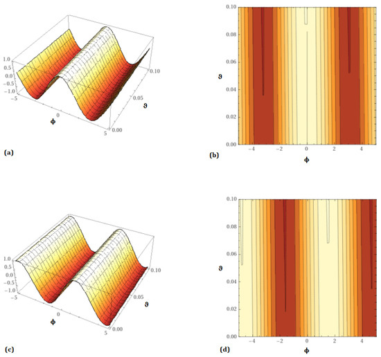
Figure 1.
Aspects of the analytical result of problem 1 in 3D and its contour for and (a) Real part, (b) Real part contour, (c) Imaginary part, and (d) Imaginary part contour.
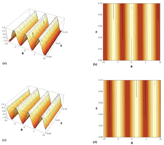
Figure 2.
Aspects of the analytical result of problem 2 in 3D and its contour for and (a) Real part, (b) Real part contour, (c) Imaginary part, and (d) Imaginary part contour.
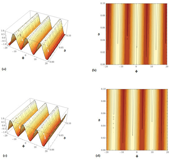
Figure 3.
Aspects of the analytical result of problem 3 in 3D and its contour for and (a) Real part, (b) Real part contour, (c) Imaginary part, and (d) Imaginary part contour.
5. Conclusions
With the use of the HPTM, the approximate and analytical solutions to the fractional Biswas–Milovic equations are successfully achieved in this study. Numerous domains, including communications, all-optical rapid switching devices, nonlinear fibre optics, and others, analyse the Biswas–Milovic equation. Many phenomena in biology, fluid flow, economics, control theory, chemistry, the life sciences, and other branches of research and engineering may now be well described using fractional calculus. An accurate simulation of a physical phenomenon depends on both the current time and the past time history. Fractional calculus can be used in this regard. Therefore, science and engineering may benefit from any new solutions to fractional equations. This paper’s main contribution is to offer a straightforward, trustworthy, and effective solution method for challenging fractional partial differential equations. The results obtained with this innovative approaches have greater accuracy in the numerical results and take less time and computational effort.
Author Contributions
Conceptualization, M.N. and P.S.; methodology, N.A.S.; software, R.S.; validation, N.A.S.; formal analysis, N.A.S.; investigation, M.N.; resources, R.S.; data curation, J.D.C.; writing—original draft preparation, M.N.; writing—review and editing, P.S.; visualization, J.D.C.; supervision, J.D.C.; project administration, M.N.; funding acquisition, J.D.C. All authors have read and agreed to the published version of the manuscript.
Funding
This research received no external funding.
Institutional Review Board Statement
Not applicable.
Informed Consent Statement
Not applicable.
Data Availability Statement
Not applicable.
Acknowledgments
The authors would like to thank the Deanship of Scientific Research at Umm Al-Qura University for supporting this work under Grant Code number: 22UQU4310396DSR51. This work was supported by a Korea Institute of Energy Technology Evaluation and Planning (KETEP) grant funded by the Korea government (MOTIE) (No. 20192010107020, Development of hybrid adsorption chiller using unutilized heat source of low temperature).
Conflicts of Interest
The authors declare no conflict of interest.
References
- Goyal, M.; Baskonus, H.M.; Prakash, A. An efficient technique for a time fractional model of lassa hemorrhagic fever spreading in pregnant women. Eur. Phys. J. Plus 2019, 134, 482. [Google Scholar] [CrossRef]
- Prakash, A.; Kumar, M.; Baleanu, D. A new iterative technique for a fractional model of nonlinear Zakharov-Kuznetsov equations via Sumudu transform. Appl. Math. Comput. 2018, 334, 30–40. [Google Scholar] [CrossRef]
- Prakash, A.; Kaur, H. A reliable numerical algorithm for fractional model of Fitzhugh-Nagumo equation arising in the transmission of nerve impulses. Nonlinear Eng.-Model. Appl. 2019, 8, 719–727. [Google Scholar] [CrossRef]
- Prakash, A.; Veeresha, P.; Prakasha, D.G.; Goyal, M. A homotopy technique for a fractional order multi-dimensional telegraph equation via the Laplace transform. Eur. Phys. J. Plus 2019, 134, 1–18. [Google Scholar] [CrossRef]
- Yang, D.; Zhu, T.; Wang, S.; Wang, S.; Xiong, Z. LFRSNet: A Robust Light Field Semantic Segmentation Network Combining Contextual and Geometric Features. Front. Environ. Sci. 2022, 1443. [Google Scholar] [CrossRef]
- Lv, Z.; Chen, D.; Feng, H.; Wei, W.; Lv, H. Artificial Intelligence in Underwater Digital Twins Sensor Networks. ACM Trans. Sen. Netw. 2022, 18, 39. [Google Scholar] [CrossRef]
- Lv, Z.; Chen, D.; Lv, H. Smart City Construction and Management by Digital Twins and BIM Big Data in COVID-19 Scenario. ACM Trans. Multimed. Comput. Commun. Appl. 2022, 18, 117. [Google Scholar] [CrossRef]
- Kovalnogov, V.N.; Fedorov, R.V.; Chukalin, A.V.; Simos, T.E.; Tsitouras, C. Eighth Order Two-Step Methods Trained to Perform Better onKeplerian-Type Orbits. Mathematics 2021, 9, 3071. [Google Scholar] [CrossRef]
- Kovalnogov, V.N.; Fedorov, R.V.; Generalov, D.A.; Chukalin, A.V.; Katsikis, V.N.; Mourtas, S.D.; Simos, T.E. Portfolio Insurance through Error-Correction Neural Networks. Mathematics 2022, 10, 3335. [Google Scholar] [CrossRef]
- Sun, L.; Hou, J.; Xing, C.; Fang, Z. A Robust Hammerstein-Wiener Model Identification Method for Highly Nonlinear Systems. Processes 2022, 10, 2664. [Google Scholar] [CrossRef]
- Young, G.O. Definition of physical consistent damping laws with fractional derivatives. Z. Angew. Math. Mech. 1995, 75, 623–635. [Google Scholar]
- He, J.H. Some applications of nonlinear fractional differential equations and their approximations. Bull. Sci. Technol. 1999, 15, 86–90. [Google Scholar]
- He, J.H. Approximate analytic solution for seepage flow with fractional derivatives in porous media. Comput. Methods Appl. Mech. Eng. 1998, 167, 57–68. [Google Scholar] [CrossRef]
- Hilfer, R. (Ed.) Applications of Fractional Calculus in Physics; World Scientific Publishing Company: Singapore, 2000; pp. 87–130. [Google Scholar]
- Mainardi, F.; Luchko, Y.; Pagnini, G. The fundamental solution of the space-time fractional diffusion equation. Frac. Calcul. Appl. Anal. 2001, 4, 153–192. [Google Scholar]
- Kilbas, A.A.; Srivastava, H.M.; Trujillo, J.J. Theory and Applications of Fractional Differential Equations; Elsevier: Amsterdam, The Netherlands, 2006. [Google Scholar]
- Lu, S.; Guo, J.; Liu, S.; Yang, B.; Liu, M.; Yin, L.; Zheng, W. An Improved Algorithm of Drift Compensation for Olfactory Sensors. Appl. Sci. 2022, 12, 9529. [Google Scholar] [CrossRef]
- Dang, W.; Guo, J.; Liu, M.; Liu, S.; Yang, B.; Yin, L.; Zheng, W. A Semi-Supervised Extreme Learning Machine Algorithm Based on the New Weighted Kernel for Machine Smell. Appl. Sci. 2022, 12, 9213. [Google Scholar] [CrossRef]
- Lu, S.; Yin, Z.; Liao, S.; Yang, B.; Liu, S.; Liu, M.; Zheng, W. An asymmetric encoder-decoder model for Zn-ion battery lifetime prediction. Energy Rep. 2022, 8, 33–50. [Google Scholar] [CrossRef]
- Ban, Y.; Liu, M.; Wu, P.; Yang, B.; Liu, S.; Yin, L.; Zheng, W. Depth Estimation Method for Monocular Camera Defocus Images in Microscopic Scenes. Electronics 2022, 11, 2012. [Google Scholar] [CrossRef]
- He, J.H. Homotopy perturbation technique. Compt. Meth. Appl. Mech. Eng. 1999, 178, 257–262. [Google Scholar] [CrossRef]
- He, J.H. A new perturbation technique which is also valid for large parameters. J. Sou. Vib. 2000, 229, 1257–1263. [Google Scholar] [CrossRef]
- Rashidi, M.M.; Ganji, D.D.; Dinarvand, S. Explicit analytical solutions of the generalized Burger and Burger-Fisher equations by homotopy perturbation method. Numer. Meth. 2009, 25, 409–417. [Google Scholar] [CrossRef]
- Rashidi, M.M.; Ganji, D.D. Homotopy Perturbation Combined with Padé Approximation for Solving Two Dimensional Viscous Flow in the Extrusion Process. Inter. J. Nonlinear Sci. 2009, 7, 387–394. [Google Scholar]
- Yildirim, A. An algorithm for solving the fractional nonlinear Schrödinger equation by means of the homotopy perturbation method. Int. J. Nonlinear Sci. Numer. Simul. 2009, 10, 445–451. [Google Scholar] [CrossRef]
- Kumar, S.; Singh, O.P. Numerical Inversion of the Abel Integral Equation using Homotopy Perturbation Method. Z. Naturforschung 2010, 65a, 677–682. [Google Scholar] [CrossRef]
- Adomian, G. Solutions of Nonlinear P.D.E. Appl. Math. Lett. 1998, 11, 121–123. [Google Scholar] [CrossRef]
- Adomian, G. Analytical solution of Navier-Stokes flow of a viscous compressible fluid. Found. Phys. Lett. 1995, 8, 389–400. [Google Scholar] [CrossRef]
- Inc, M.; Cherruault, Y. A new approach to solve a diffusion-convection problem. Kybernetes 2002, 31, 536–549. [Google Scholar] [CrossRef]
- Basto, M.; Semiao, V.; Calheiros, F.L. Numerical study of modified Adomian’s method applied to Burgers equation. J. Comput. Appl. Math. 2007, 206, 927–949. [Google Scholar] [CrossRef]
- Krasnoschok, M.; Pata, V.; Siryk, S.V.; Vasylyeva, N. A subdiffusive Navier-Stokes-Voigt system. Phys. D Nonlinear Phenom. 2020, 409, 132503. [Google Scholar] [CrossRef]
- Gu, W.; Wei, F.; Li, M. Parameter Estimation for a Type of Fractional Diffusion Equation Based on Compact Difference Scheme. Symmetry 2022, 14, 560. [Google Scholar] [CrossRef]
- Krasnoschok, M.; Pereverzyev, S.; Siryk, S.V.; Vasylyeva, N. Regularized reconstruction of the order in semilinear subdiffusion with memory. Springer Proc. Math. Stat. 2020, 310, 205–236. [Google Scholar]
- Jin, B.; Kian, Y.; Zhou, Z. Reconstruction of a space-time-dependent source in subdiffusion models via a perturbation approach. SIAM J. Math. Anal. 2021, 53, 4445–4473. [Google Scholar] [CrossRef]
- Krasnoschok, M.; Pereverzyev, S.; Siryk, S.V.; Vasylyeva, N. Determination of the fractional order in semilinear subdiffusion equations. Fract. Calc. Appl. Anal. 2020, 23, 694–722. [Google Scholar] [CrossRef]
- Ahmad, S.; Ullah, A.; Akgul, A.; De la Sen, M. A Novel Homotopy Perturbation Method with Applications to Nonlinear Fractional Order KdV and Burger Equation with Exponential-Decay Kernel. J. Funct. Spaces 2021, 2021, 8770488. [Google Scholar] [CrossRef]
- Xu, Y. Similarity solution and heat transfer characteristics for a class of nonlinear convection-diffusion equation with initial value conditions. Math. Probl. Eng. 2019, 2019, 3467276. [Google Scholar] [CrossRef]
- Sun, H.; Zhang, Y.; Baleanu, D.; Chen, W.; Chen, Y. A new collection of real world applications of fractional calculus in science and engineering. Commun. Nonlinear Sci. Numer. Simulat. 2018, 64, 213–231. [Google Scholar] [CrossRef]
- Krasnoschok, M.; Pata, V.; Siryk, S.V.; Vasylyeva, N. Equivalent definitions of Caputo derivatives and applications to subdiffusion equations. Dyn. Partial. Differ. Equ. 2020, 17, 383–402. [Google Scholar] [CrossRef]
- Diethelm, K.; Garrappa, R.; Stynes, M. Good (and Not So Good) practices in computational methods for fractional calculus. Mathematics 2020, 8, 324. [Google Scholar] [CrossRef]
- Alaoui, M.K.; Fayyaz, R.; Khan, A.; Shah, R.; Abdo, M.S. Analytical investigation of Noyes-Field model for time-fractional Belousov-Zhabotinsky reaction. Complexity 2021, 2021, 3248376. [Google Scholar] [CrossRef]
- Qin, Y.; Khan, A.; Ali, I.; Al Qurashi, M.; Khan, H.; Shah, R.; Baleanu, D. An efficient analytical approach for the solution of certain fractional-order dynamical systems. Energies 2020, 13, 2725. [Google Scholar] [CrossRef]
- Nonlaopon, K.; Alsharif, A.M.; Zidan, A.M.; Khan, A.; Hamed, Y.S.; Shah, R. Numerical investigation of fractional-order Swift-Hohenberg equations via a Novel transform. Symmetry 2021, 13, 1263. [Google Scholar] [CrossRef]
- Khan, H.; Khan, A.; Kumam, P.; Baleanu, D.; Arif, M. An approximate analytical solution of the Navier-Stokes equations within Caputo operator and Elzaki transform decomposition method. Adv. Differ. Equ. 2020, 2020, 1–23. [Google Scholar]
- Khan, H.; Khan, A.; Al-Qurashi, M.; Shah, R.; Baleanu, D. Modified modelling for heat like equations within Caputo operator. Energies 2020, 13, 2002. [Google Scholar] [CrossRef]
- Dehghan, M.; Manafian, J.; Saadatmandi, A. Solving nonlinear fractional partial differential equations using the homotopy analysis method. Numer. Methods Partial. Differ. Equ. Int. J. 2010, 26, 448–479. [Google Scholar] [CrossRef]
- Alderremy, A.A.; Aly, S.; Fayyaz, R.; Khan, A.; Shah, R.; Wyal, N. The Analysis of Fractional-Order Nonlinear Systems of Third Order KdV and Burgers Equations via a Novel Transform. Complexity 2022, 2022, 4935809. [Google Scholar] [CrossRef]
- Areshi, M.; Khan, A.; Shah, R.; Nonlaopon, K. Analytical investigation of fractional-order Newell-Whitehead-Segel equations via a novel transform. Aims Math. 2022, 7, 6936–6958. [Google Scholar] [CrossRef]
- Biswas, A.; Milovic, D. Bright and dark solitons of the generalized nonlinear Schrodinger’s equation. Commun. Nonlinear Sci. Numer. Simul. 2010, 15, 1473–1484. [Google Scholar] [CrossRef]
- Ahmed, I.; Mu, C.; Zhang, F. Exact solution of the Biswas-Milovic equation by Adomian decomposition method. Int. J. Appl. Math. Res. 2013, 2, 418–422. [Google Scholar] [CrossRef]
- Mirzazadeh, M.; Arnous, A.H. Exact solution of Biswas- Milovic equation using new efficient method. Elec. J. Math. Anal. Appl. 2015, 3, 139–146. [Google Scholar]
- Ahmadian, S.; Darvishi, M.T. A new fractional Biswas-Milovic model with its periodic soliton solutions. Optik 2016, 127, 7694–7703. [Google Scholar] [CrossRef]
- Ahmadian, S.; Darvishi, M.T. fractional version of (1+1) dimensional Biswas-Milovic equation and its solutions. Optik 2016, 127, 10135–10147. [Google Scholar] [CrossRef]
- Zaidan, L.I.; Darvishi, M.T. Semi-analytical solutions of different kinds of fractional Biswas-Milovic equation. Optik 2017, 136, 403–410. [Google Scholar] [CrossRef]
- Singh, J.; Kumar, D.; Baleanu, D. New aspects of fractional Biswas-Milovic model with Mittag-Leffler law. Math. Model. Nat. Phenom. 2019, 14, 303. [Google Scholar] [CrossRef]
- Saad Alshehry, A.; Imran, M.; Khan, A.; Shah, R.; Weera, W. Fractional View Analysis of Kuramoto-Sivashinsky Equations with Non-Singular Kernel Operators. Symmetry 2022, 14, 1463. [Google Scholar] [CrossRef]
- Sunthrayuth, P.; Alyousef, H.A.; El-Tantawy, S.A.; Khan, A.; Wyal, N. Solving Fractional-Order Diffusion Equations in a Plasma and Fluids via a Novel Transform. J. Funct. Spaces 2022, 2022, 1899130. [Google Scholar] [CrossRef]
- Ghorbani, A. Beyond Adomian polynomials: He polynomials. Chaos Solitons Fractals 2009, 39, 1486–1492. [Google Scholar] [CrossRef]
Disclaimer/Publisher’s Note: The statements, opinions and data contained in all publications are solely those of the individual author(s) and contributor(s) and not of MDPI and/or the editor(s). MDPI and/or the editor(s) disclaim responsibility for any injury to people or property resulting from any ideas, methods, instructions or products referred to in the content. |
© 2023 by the authors. Licensee MDPI, Basel, Switzerland. This article is an open access article distributed under the terms and conditions of the Creative Commons Attribution (CC BY) license (https://creativecommons.org/licenses/by/4.0/).