Dynamical Properties, Deformations, and Chaos in a Class of Inversion Invariant Jerk Equations

Abstract

In this paper, we consider a class of jerk equations which are invariant to inversion. We discuss the stability and some bifurcations of the considered equation. In addition, we construct integrable deformations in order to stabilize some equilibrium points. Finally, we introduce a piecewise chaotic system which belongs to the considered class of jerk equations.

1. Introduction

A third-order autonomous ordinary differential equation that contains the third time derivative of position, called jerk [1], is known as a jerk equation. Denoting by $x=x\left(t\right)$ the position at the moment t, the explicit form of a jerk equation is $\stackrel{⃛}{x}=j(x,\dot{x},\ddot{x}),$ where over-dots stand for time derivatives and j is the jerk function (see, e.g., [2] and references therein). Jerk equations have several applications in engineering (see, e.g., [1] and references therein). In addition, many jerk equations with chaotic behavior have been reported (see, e.g., [3,4,5,6,7,8]).

A jerk equation is written in an equivalent form as a three-dimensional system of autonomous differential equations, namely $\dot{x}=y,\dot{y}=z,\dot{z}=j(x,y,z),$ which allows for studying some geometric symmetries and dynamical behavior. Moreover, integrable deformations of such a jerk system can be constructed (see, e.g., [9,10]).

Several papers which deal with chaotic jerk equations have as a starting point the jerk equation introduced in [3], namely $\stackrel{⃛}{x}+\beta \ddot{x}+\dot{x}=f_{\mu }\left(x\right),$ where $\beta >0$ is the dissipation and $\mu$ is a real parameter of the function $f_{\mu }$. As specified in [3], this jerk equation is the compact form of $\ddot{x}+\beta \dot{x}+x=\eta ,\dot{\eta }=f_{\mu }\left(x\right).$ A mechanism to obtain this system is as follows. Consider the particular harmonic oscillator $\ddot{x}+x=0$, and its damped version $\ddot{x}+\beta \dot{x}+x=0,$ where $\beta >0$ is the dissipation. Then, the above-mentioned system is obtained applying an external force $\eta =\eta (x,\mu )$ with the property $\dot{\eta }=f_{\mu }\left(x\right)$. In the same manner, we consider the differential equation describing a particle in some potential $V=V\left(x\right)$ (see, e.g., [11,12,13] and references therein) that is $\ddot{x}+V^{\prime }\left(x\right)=0$. Using the same damping and external force, we obtain the following class of jerk equations:

$$\stackrel{⃛}{x}+\beta \ddot{x}+V^{″}\left(x\right)\dot{x}=f_{\mu }\left(x\right),$$

(1)

where

$$\beta >0,\mu \in \mathbb{R},$$

(2)

or, in equivalent form,

$$\left\{\begin{array}{c}\dot{x}=y\hfill \\ \dot{y}=z\hfill \\ \dot{z}=f_{\mu }\left(x\right)-V^{″}\left(x\right)y-\beta z\hfill \end{array}\right..$$

(3)

The paper is organized as follows: in Section 2, we establish conditions for which the considered jerk equation is invariant with respect to the inversion $(x,y,z)\to (-x,-y,-z)$. Under these conditions, in Section 3, we discuss the stability and some bifurcations of system (3). In addition, we analyze a particular case of this system which has a double-fork symmetrical bifurcation diagram of equilibrium points. In Section 4, we construct a family of deformations of the considered system which is also invariant with respect to the same transformation. Moreover, we give conditions so that equilibrium points of the initial system are stabilized. In Section 5, we introduce a chaotic piecewise jerk equation of the form (1). In Section 6, the conclusions are presented.

2. Symmetries

In this section, we discuss a jerk equation and, in particular, system (3) by a geometric symmetries point of view. More precisely, we give conditions such that a jerk equation is invariant under certain transformations and we notice that it cannot be invariant in the case of others. First, we recall some notions regarding such symmetries (for details, see e.g., [14,15,16]).

A set of points in the three-dimensional space has symmetry if it is invariant under some transformation. Particularly, the invariance with respect to changing the sign of three, two, and one variable leads to the existence of a center, an axis, and a plane of symmetry, respectively. More exactly, the origin $O(x,y,z)$ is a center of symmetry of a set of points, if this set is invariant under the transformation $(x,y,z)\to (-x,-y,-z)$. The z-axis is an axis of symmetry if the set is invariant under the transformation $(x,y,z)\to (-x,-y,z)$. In this case, the set is invariant with respect to a ${180}^{\circ }$ rotation about the z-axis; thus, it has a rotational symmetry. Finally, if the set is invariant under the transformation $(x,y,z)\to (x,y,-z),$ then the $z=0$ plane is a plane of symmetry (reflection plane) for the considered set of points. All above-mentioned transformations that is inversion, rotation, and reflection, respectively, are elementary involutional symmetries, and they can be considered in the case of three-dimensional systems of autonomous first-order ordinary differential equations in the variables $x,$ $y,$ and z (see, e.g., [16]). The invariance of a system with respect to such a transformation leads to a symmetrical orbit or a pair of symmetrical orbits corresponding to symmetrical initial conditions.

Let us return to the jerk system

$$\left\{\begin{array}{c}\dot{x}=y\hfill \\ \dot{y}=z\hfill \\ \dot{z}=j(x,y,z)\hfill \end{array}\right..$$

(4)

Consider the linear transformation $T:{\mathbb{R}}^3\to {\mathbb{R}}^3,$ $T(x,y,z)=(ax,by,cz)$, where $a,b,c\in \{-1,1\}$, which is not the identity. Applying T to system (4), we obtain

$$\left\{\begin{array}{c}a\dot{x}=by\hfill \\ b\dot{y}=cz\hfill \\ c\dot{z}=j(ax,by,cz)\hfill \end{array}\right..$$

(5)

System (4) is invariant under the transformation T if system (5) is identical with (4). It follows that $a=b=c$ and $j(ax,by,cz)=cj(x,y,z),$ for all $x,y,z$. Hence, $a=b=c=-1.$ Therefore, system (4) cannot have a rotation or a reflection symmetry. Moreover, the above jerk system is invariant with respect to the inversion $(x,y,z)\to (-x,-y,-z)$ if and only if $j(-x,-y,-z)=-j(x,y,z)$ for all $x,y,z$.

Remark 1.

If the functions V and $f_{\mu }$ satisfy $V^{″}(-x)=V^{″}\left(x\right),f_{\mu }(-x)=-f_{\mu }\left(x\right)$ for all x, then jerk system (3) is an inversion invariant system.

3. Stability and Bifurcations

In this section, we study the stability of system (3) under the conditions given by Remark 1. We present sufficient conditions such that the considered system experiences a zero bifurcation. Furthermore, we point out some bifurcations of the inversion invariant system (3). Finally, we study a particular case of the considered system.

In the first two results, we discuss the equilibrium points of system (3) and their stability under the conditions given by Remark 1.

Proposition 1.

Let $f_{\mu }:\mathbb{R}\to \mathbb{R}$ be an odd function. Then:

(a) 

The equilibrium points of system (3) are $E(x_0,0,0)$, where $x_0\in \mathbb{R}$ is a solution of equation $f_{\mu }\left(x\right)=0;$

(b) 

$O(0,0,0)$ is an equilibrium point of system (3);

(c) 

If $x_1\ne 0$ is a solution of equation $f_{\mu }\left(x\right)=0$, then $E_1^{\pm }(\pm x_1,0,0)$ are equilibrium points of system (3).

Proof. 

The equilibrium points $E(x,y,z)$ are the solutions of the system

$$y=0,z=0,f_{\mu }\left(x\right)-V^{″}\left(x\right)y-\beta z=0,$$

which proves (a). In addition, $f_{\mu }$ is an odd function and the other conclusions follow. □

Proposition 2.

Let $f_{\mu }:\mathbb{R}\to \mathbb{R}$ be an odd function and $V:\mathbb{R}\to \mathbb{R}$ such that $V^{″}$ is an even function. Denote by $E(x_0,0,0)$ an equilibrium point of system (3).

(a) 

If $V^{″}\left(x_0\right)>0$ and $-\beta V^{″}\left(x_0\right)<f_{\mu }^{\prime }\left(x_0\right)<0,$ then E is asymptotically stable.

(b) 

If $V^{″}\left(x_0\right)<0$ or $f_{\mu }^{\prime }\left(x_0\right)>0$ or $f_{\mu }^{\prime }\left(x_0\right)<-\beta V^{″}\left(x_0\right),$ then E is unstable.

(c) 

If $V^{″}\left(x_0\right)=0$ and $f_{\mu }^{\prime }\left(x_0\right)<0,$ then E is unstable.

Proof. 

The Jacobian matrix J of system (3), given by

$$J(x,y,z)=\left[\begin{array}{ccc}0& 1& 0\\ 0& 0& 1\\ f_{\mu }^{\prime }\left(x\right)-V^{″\prime }\left(x\right)y& -V^{″}\left(x\right)& -\beta \end{array}\right],$$

(6)

where $f_{\mu }^{\prime }\left(x\right)=\frac{d{f}_{\mu }}{dx}\left(x\right)$ leads to the characteristic polynomial associated with the equilibrium point E,

$$P_E\left(\lambda \right)={\lambda }^3+\beta {\lambda }^2+V^{″}\left(x_0\right)\lambda -f_{\mu }^{\prime }\left(x_0\right).$$

(7)

Assertions (a) and (b) are direct consequences of the Routh–Hurwitz theorem (see, e.g., [17]) and First Lyapunov’s stability criterion [18]. More precisely, if the conditions in (a) are fulfilled, then all the roots of the characteristic polynomial have a negative real part and consequently the equilibrium point E is asymptotically stable. On the other hand, any condition in (b) implies that $P_E\left(\lambda \right)$ has at least one root with a strictly positive real part, that is, E is an unstable equilibrium point.

For (c), we observe that $P_E(-\beta )>0$; thus, a real root of $P_E\left(\lambda \right)$ is ${\lambda }_1<-\beta <0.$ It is easy to see that the function $P_E\left(\lambda \right)$ has the local minimum point $\lambda =-\frac{2}{3}\beta$ with $P_E(-\frac{2}{3}\beta )>0$ and the local maximum point $\lambda =0$ with $P_E\left(0\right)>0$. Using the monotony of the function $P_E\left(\lambda \right)$, it follows that its other two roots ${\lambda }_{2,3}$ are complex numbers. Since ${\lambda }_2+{\lambda }_3=-{\lambda }_1-\beta >0$, we obtain Re$\left({\lambda }_{2,3}\right)>0,$ which finishes the proof. □

Remark 2.

In the cases considered in Proposition 2, the equilibrium points are hyperbolic. In the other cases, the equilibrium points are non-hyperbolic, and some bifurcations can occur in the dynamics of system (3). More precisely, in the case $V^{″}\left(x_0\right)>0$ and $f_{\mu }^{\prime }\left(x_0\right)=0,$ a root of $P_E\left(\lambda \right)$ is ${\lambda }_1=0$ and the other two have negative real parts. Using the Local center manifold theorem (see, e.g., [19]), the stability of the considered equilibrium point may be deduced. Moreover, considering μ as a parameter of bifurcation, the system may display a zero bifurcation (a generic saddle–node bifurcation, a transcritical or a pitchfork bifurcation; see, e.g., [20]).

In the case $V^{″}\left(x_0\right)>0,f_{\mu }^{\prime }\left(x_0\right)=-\beta V^{″}\left(x_0\right)$, it is easy to see that the roots of $P_E\left(\lambda \right)$ are ${\lambda }_1=-\beta <0$ and ${\lambda }_{2,3}=\pm i\sqrt{V^{″}\left(x_0\right)},$ and consequently a Hopf bifurcation may occur in the dynamics of the considered system. In addition, the reduction on the local center manifold may establish if the equilibrium point is stable or not (see, e.g., [21]).

Finally, if $V^{″}\left(x_0\right)=0$ and $f_{\mu }^{\prime }\left(x_0\right)=0,$ then ${\lambda }_1=-\beta <0,{\lambda }_2={\lambda }_3=0.$ If a second parameter is introduced in the system, then a double-zero bifurcation or Bogdanov–Takens bifurcation may arise (see, e.g., [21]).

In the following, we analyze the above-mentioned bifurcations using the Sotomayor theorem [22] (see also [19,20]). Notice that system (3) has the form $(\dot{x},\dot{y},\dot{z})=(F(x,y,z,\mu ),G(x,y,z,\mu ),H(x,y,z,\mu )),$ that is $\dot{\mathbf{x}}=\mathbf{f}(\mathbf{x},\mu ),$ where $\mu$ is a real parameter.

Proposition 3.

Let $E(x_0,0,0)$ be an equilibrium point of system (3) and let ${\mu }_0\in \mathbb{R}$ be the critical parameter value of bifurcation such that $V^{″}\left(x_0\right)>0$ and $f_{{\mu }_0}^{\prime }\left(x_0\right)=0.$ Then:

(a) 

$D_{\mathbf{x}}\mathbf{f}(E,{\mu }_0)=J\left(E\right){|}_{\mu ={\mu }_0}$ (6) has a simple eigenvalue 0 with right eigenvector ${\mathbf{v}}^t=(1,0,0)$ and left eigenvector ${\mathbf{w}}^t=(-V^{″}\left(x_0\right),\beta ,1);$

(b) 

${\displaystyle \frac{\partial \mathbf{f}}{\partial \mu }}(E,{\mu }_0)=\left(0,0,{\displaystyle \frac{\partial f_{\mu }}{\partial \mu }}\left(x_0\right){|}_{\mu ={\mu }_0}\right)$ and ${\mathbf{w}}^t·{\displaystyle \frac{\partial \mathbf{f}}{\partial \mu }}(E,{\mu }_0)={\displaystyle \frac{\partial f_{\mu }}{\partial \mu }}\left(x_0\right){|}_{\mu ={\mu }_0};$

(c) 

$D_{\mathbf{x}}^2\mathbf{f}(E,{\mu }_0)\left(\mathbf{v},\mathbf{v}\right)=(0,0,f_{{\mu }_0}^{″}\left(x_0\right))$ and ${\mathbf{w}}^t·D_{\mathbf{x}}^2\mathbf{f}(E,{\mu }_0)\left(\mathbf{v},\mathbf{v}\right)=f_{{\mu }_0}^{″}\left(x_0\right);$

(d) 

${\displaystyle \frac{\partial {\mathbf{D}}_{\mathbf{x}}\mathbf{f}}{\partial \mu }}(E,{\mu }_0)\left(\mathbf{v}\right)=\left(0,0,{\displaystyle \frac{\partial f_{\mu }^{\prime }}{\partial \mu }}\left(x_0\right){|}_{\mu ={\mu }_0}\right)$ and ${\mathbf{w}}^t·{\displaystyle \frac{\partial {\mathbf{D}}_{\mathbf{x}}\mathbf{f}}{\partial \mu }}(E,{\mu }_0)\left(\mathbf{v}\right)={\displaystyle \frac{\partial f_{\mu }^{\prime }}{\partial \mu }}\left(x_0\right){|}_{\mu ={\mu }_0}$;

(e) 

$D_{\mathbf{x}}^3\mathbf{f}(E,{\mu }_0)\left(\mathbf{v},\mathbf{v},\mathbf{v}\right)=(0,0,f_{{\mu }_0}^{″\prime }\left(x_0\right))$ and ${\mathbf{w}}^t·D_{\mathbf{x}}^3\mathbf{f}(E,{\mu }_0)\left(\mathbf{v},\mathbf{v},\mathbf{v}\right)=f_{{\mu }_0}^{″\prime }\left(x_0\right),$ where “·” stands for a dot product.

Proof. 

The conclusions follow by simple computations, where

$D_{\mathbf{x}}^2\mathbf{f}\left(\mathbf{v},\mathbf{v}\right)=(d^{2}F\left(\mathbf{v},\mathbf{v}\right),d^{2}G\left(\mathbf{v},\mathbf{v}\right),d^{2}H\left(\mathbf{v},\mathbf{v}\right))$, $D_{\mathbf{x}}^3\mathbf{f}\left(\mathbf{v},\mathbf{v},\mathbf{v}\right)=(d^{3}F\left(\mathbf{v},\mathbf{v},\mathbf{v}\right),d^{3}G\left(\mathbf{v},\mathbf{v},\mathbf{v}\right),d^{3}H\left(\mathbf{v},\mathbf{v},\mathbf{v}\right)).$ □

The condition in which some dot products calculated in Proposition 3 vanish or not ensures which kind of zero bifurcation occurs in system (3). More precisely, following [19], Sotomayor’s conditions in our case are as follows.

Proposition 4.

Let $E(x_0,0,0)$ be an equilibrium point of system (3) and let ${\mu }_0\in \mathbb{R}$ be the critical parameter value of bifurcation such that $V^{″}\left(x_0\right)>0$ and $f_{{\mu }_0}^{\prime }\left(x_0\right)=0.$

(a) 

If ${\displaystyle \frac{\partial f_{\mu }}{\partial \mu }}\left(x_0\right){|}_{\mu ={\mu }_0}\ne 0,f_{{\mu }_0}^{″}\left(x_0\right)\ne 0,$ then system (3) experiences a saddle-node bifurcation at the equilibrium point E as the parameter μ passes through the bifurcation value ${\mu }_0.$

(b) 

If ${\displaystyle \frac{\partial f_{\mu }}{\partial \mu }}\left(x_0\right){{|}_{\mu ={\mu }_0}=0,f_{{\mu }_0}^{″}\left(x_0\right)\ne 0,{\displaystyle \frac{\partial f_{\mu }^{\prime }}{\partial \mu }}\left(x_0\right)|}_{\mu ={\mu }_0}\ne 0,$ then system (3) experiences a transcritical bifurcation at the equilibrium point E as the parameter μ passes through the bifurcation value ${\mu }_0.$

(c) 

If ${\displaystyle \frac{\partial f_{\mu }}{\partial \mu }}\left(x_0\right){{|}_{\mu ={\mu }_0}=0,f_{{\mu }_0}^{″}\left(x_0\right)=0,{\displaystyle \frac{\partial f_{\mu }^{\prime }}{\partial \mu }}\left(x_0\right)|}_{\mu ={\mu }_0}\ne 0,f_{{\mu }_0}^{″\prime }\left(x_0\right)\ne 0,$ then system (3) experiences a pitchfork bifurcation at the equilibrium point E as the parameter μ passes through the bifurcation value ${\mu }_0.$

Now, we discuss bifurcations of the inversion invariant system (3).

Proposition 5.

Let $f_{\mu }:\mathbb{R}\to \mathbb{R}$ be an odd function and $V:\mathbb{R}\to \mathbb{R}$ such that $V^{″}$ is an even function. Let ${\mu }_0\in \mathbb{R}$ be the critical parameter value of bifurcation such that $V^{″}\left(0\right)>0$ and $f_{{\mu }_0}^{\prime }\left(0\right)=0.$ Then, a saddle-node bifurcation or a transcritical bifurcation cannot occur in system (3) at the equilibrium point $O(0,0,0).$

Moreover, if ${\displaystyle \frac{\partial f_{\mu }^{\prime }}{\partial \mu }}{\left(0\right)|}_{\mu ={\mu }_0}\ne 0$ and $f_{{\mu }_0}^{″\prime }\left(0\right)\ne 0,$ then system (3) displays a pitchfork bifurcation at $O.$

Proof. 

Because $f_{\mu }$ is an odd function, it follows ${\displaystyle \frac{\partial f_{\mu }}{\partial \mu }}{\left(0\right)|}_{\mu ={\mu }_0}=0$ and $f_{{\mu }_0}^{″}\left(0\right)=0,$ that is, both transversality conditions of the saddle-node bifurcation are violated (see Proposition 4). In addition, one of the transversality conditions of the transcritical bifurcation is also violated. Therefore, these bifurcations cannot occur in system (3) at O. Under the hypothesis, the transversality conditions of the pitchfork bifurcation are fulfilled, as required.  □

Remark 3.

As we have seen in Proposition 1, O is always an equilibrium point of system (3) and other points appear as pairs $E^{\pm }$, provided they exist. In the case of a pitchfork bifurcation, three equilibrium points, O, $E^{+}$, and $E^{-}$ in our case, coalesce into one, namely O. Moreover, the stability of O changes in $\mu ={\mu }_0.$

In the next result, we point out sufficient conditions for our system to display a Hopf bifurcation (according to Hopf’s theorem; see, e.g., [20]).

Proposition 6.

Let $f_{\mu }:\mathbb{R}\to \mathbb{R}$ be an odd function and $V:\mathbb{R}\to \mathbb{R}$ such that $V^{″}$ is an even function. Let $E(x_0,0,0)$ be an equilibrium point of system (3) and let ${\mu }_0\in \mathbb{R}$ be the critical parameter value of bifurcation such that $V^{″}\left(x_0\right)>0$ and $f_{{\mu }_0}^{\prime }\left(x_0\right)=-\beta V^{″}\left(x_0\right).$ If ${\displaystyle \frac{\partial f_{\mu }^{\prime }}{\partial \mu }}\left(x_0\right){|}_{\mu ={\mu }_0}\ne 0,$ then system (3) displays a Hopf bifurcation at E.

Proof. 

If there is ${\mu }_0\in \mathbb{R}$ such that $f_{{\mu }_0}^{\prime }\left(x_0\right)=-\beta V^{″}\left(x_0\right)<0,$ then the eigenvalues of the Jacobian matrix J of system (3) at E are ${\lambda }_1=-\beta <0$ and ${\lambda }_{2,3}=\pm i\sqrt{V^{″}\left(x_0\right)},$ that is the first condition in Hopf’s theorem is fulfilled. By the Implicit Function Theorem, the equation $P_E\left(\lambda \right)=0$ (7) defines the function $\lambda =\lambda \left(\mu \right)$ with the properties $\lambda \left({\mu }_0\right)=i\sqrt{V^{″}\left(x_0\right)}$ and

$${\displaystyle \frac{d\lambda }{d\mu }}\left({\mu }_0\right)=-{\left.{\displaystyle \frac{\frac{\partial P_E}{\partial \mu }\left(x_0\right)}{\frac{\partial P_E}{\partial \lambda }\left(x_0\right)}}\right|}_{\mu ={\mu }_0}={\left.{\displaystyle \frac{\frac{\partial f_{\mu }^{\prime }}{\partial \mu }\left(x_0\right)}{3{\lambda }^2+2\beta \lambda +V^{″}\left(x_0\right)}}\right|}_{\mu ={\mu }_0}={\displaystyle \frac{{\left.\frac{\partial f_{\mu }^{\prime }}{\partial \mu }\left(x_0\right)\right|}_{\mu ={\mu }_0}}{-2V^{″}\left(x_0\right)+2\beta \sqrt{V^{″}\left(x_0\right)}i}}.$$

By hypothesis, it follows that

$${\displaystyle \frac{d}{d\mu }}{\left(Re\lambda \left(\mu \right)\right)|}_{\mu ={\mu }_0}\ne 0,$$

and consequently the Hopf bifurcation occurs at E. □

We point out the above-mentioned bifurcations in the following example. We consider $\beta =1$ and the functions $V\left(x\right)=\frac{1}{2}{x}^2,$$f_{\mu }\left(x\right)=x(x^2-\mu )(x^2+\mu -2).$ System (3) writes

$$\left\{\begin{array}{c}\dot{x}=y\hfill \\ \dot{y}=z\hfill \\ \dot{z}=\mu (2-\mu )x-2x^3+x^5-y-z\hfill \end{array},\mu \in \mathbb{R}.\right.$$

(8)

Denote $O(0,0,0),E_1^{\pm }(\pm \sqrt{\mu },0,0),E_2^{\pm }(\pm \sqrt{2-\mu },0,0).$ The number of equilibrium points depends on $\mu$. More precisely, if $\mu \in (-\infty ,0]$ or $\mu \in [2,\infty )$, then there are three equilibrium points, $O,E_2^{\pm }$ and $O,E_1^{\pm }$, respectively. Moreover, if $\mu =1$, there are also three equilibrium points $O,E_1^{\pm }$ since $E_2^{+}$ collides with $E_1^{+}$ and $E_2^{-}$ with $E_1^{-}$. Otherwise, system (8) has five equilibrium points, $O,E_1^{\pm },E_2^{\pm }.$

By Proposition 2, we deduce.

Proposition 7.

Let $O(0,0,0),E_1^{\pm }(\pm \sqrt{\mu },0,0),E_2^{\pm }(\pm \sqrt{2-\mu },0,0)$ be the equilibrium points of system (8).

(a) 

If $\mu \in (1-\sqrt{2},0)\cup (2,1+\sqrt{2}),$ then O is asymptotically stable, and if $\mu \in (-\infty ,1-\sqrt{2})\cup (0,2)\cup (1+\sqrt{2},\infty ),$ it is unstable.

(b) 

$E_1^{\pm }$ is asymptotically stable for $\mu \in (0,1)\backslash \left\{\frac{1}{2}\right\}$, and unstable for $\mu \in (1,\infty ).$

(c) 

$E_2^{\pm }$ is asymptotically stable for $\mu \in (1,2)\backslash \left\{\frac{3}{2}\right\}$, and unstable for $\mu \in (-\infty ,1).$

The above results are gathered in Figure 1, where dashed and solid lines stand for instability and asymptotic stability, respectively. The non-hyperbolic cases of the equilibrium points are marked by solid circles.

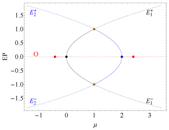
Figure 1. The bifurcation diagram for the equilibrium points of system (8) in the $\mu -x$ plane. The equilibrium points $O,E_1^{\pm },E_2^{\pm }$ are represented by red, black, and blue lines, respectively. Dashed and solid lines stand for instability and asymptotic stability, respectively. Solid dots mark the non-hyperbolic equilibrium points, which correspond to the critical values of the parameter $\mu$.

For $\mu \in \{0,2\},$ the roots of the characteristic polynomial (7) at $O(0,0,0)$ are ${\lambda }_1=0,{\lambda }_{2,3}=-\frac{1}{2}\pm \frac{i\sqrt{3}}{2}$. In addition, the stability of O changes at these values of $\mu$, which suggests a zero bifurcation. Furthermore, the reduction of system (8) on a center manifold furnishes the stability of O. We recall the three-dimensional version of this result (see, e.g., [23]).

Theorem 1

(The local center manifold theorem. [19]).Let $\mathbf{f}\in C^r(E,{\mathbb{R}}^3)$, where E is an open set of ${\mathbb{R}}^3$ containing the origin and $r\ge 1.$ Suppose that $\mathbf{f}(0,0,0)=(0,0,0)$ and that $D\mathbf{f}(0,0,0)$ has c eigenvalues with zero real parts and s eigenvalues with negative real parts, where $c+s=3,c\in \{1,2\}.$ The system $\dot{\mathbf{x}}=\mathbf{f}\left(\mathbf{x}\right)$ then can be written in diagonal form

$$\dot{\mathbf{x}}=C\mathbf{x}+\mathbf{F}(\mathbf{x},\mathbf{y}),\dot{\mathbf{y}}=P\mathbf{y}+\mathbf{G}(\mathbf{x},\mathbf{y}),$$

where $(\mathbf{x},\mathbf{y})\in {\mathbb{R}}^c\times {\mathbb{R}}^s,$ C a square matrix with c eigenvalues having zero real parts, P is a square matrix with s eigenvalues with negative real parts, and $\mathbf{F}\left(\mathbf{0}\right)=\mathbf{G}\left(\mathbf{0}\right)=\mathbf{0},D\mathbf{F}\left(\mathbf{0}\right)=D\mathbf{G}\left(\mathbf{0}\right)=O$; furthermore, there exists a $\delta >0$ and a function $\mathbf{h}\in C^r\left(N_{\delta }\left(\mathbf{0}\right)\right)$, such that $\mathbf{h}\left(\mathbf{0}\right)=\mathbf{0},D\mathbf{h}\left(\mathbf{0}\right)=O$ that defines the local center manifold

$$W^c\left(\mathbf{0}\right)=\{(\mathbf{x},\mathbf{y})\in {\mathbb{R}}^c\times {\mathbb{R}}^s|\mathbf{y}=\mathbf{h}\left(\mathbf{x}\right)for |\mathbf{x}|<\delta \}$$

(9)

and satisfies

$$D\mathbf{h}\left(\mathbf{x}\right)[C\mathbf{x}+\mathbf{F}(\mathbf{x},\mathbf{h}\left(\mathbf{x}\right)\left)\right]-P\mathbf{h}\left(\mathbf{x}\right)-\mathbf{G}(\mathbf{x},\mathbf{h}(\mathbf{x}\left)\right)=\mathbf{0}$$

(10)

for $\left|\mathbf{x}\right|<\delta$; and the flow on the center manifold $W^c\left(\mathbf{0}\right)$ is defined by the system of differential equations:

$$\dot{\mathbf{x}}=C\mathbf{x}+\mathbf{F}(\mathbf{x},\mathbf{h}\left(\mathbf{x}\right))$$

(11)

for all $\mathbf{x}\in {\mathbb{R}}^c$ with $\left|\mathbf{x}\right|<\delta$.

Now, we have:

Proposition 8.

Let $\mu \in \{0,2\}$. Then, system (8) reduces on a local center manifold to the equation $\dot{u}=-2u^3+O\left(u^5\right)$ and consequently the equilibrium point O is stable.

Proof. 

The roots of the characteristic polynomial (7) at $O(0,0,0)$ are ${\lambda }_1=0,{\lambda }_{2,3}=-\frac{1}{2}\pm \frac{i\sqrt{3}}{2}$. Then, $c=1,s=2$ in the above theorem. Using the transformation

$$x=u-\frac{1}{2}v+\frac{\sqrt{3}}{2}w,y=-\frac{1}{2}v-\frac{\sqrt{3}}{2}w,z=v,$$

we obtain the diagonal form of system (8)

$$\left\{\begin{array}{ccc}\dot{u}\hfill & =\hfill & -2{\left(u-\frac{v}{2}+\frac{\sqrt{3}w}{2}\right)}^3+{\left(u-\frac{v}{2}+\frac{\sqrt{3}w}{2}\right)}^5\hfill \\ \dot{v}\hfill & =\hfill & -\frac{v}{2}+\frac{\sqrt{3}w}{2}-2{\left(u-\frac{v}{2}+\frac{\sqrt{3}w}{2}\right)}^3+{\left(u-\frac{v}{2}+\frac{\sqrt{3}w}{2}\right)}^5\hfill \\ \dot{w}\hfill & =\hfill & -\frac{\sqrt{3}}{2}v-\frac{w}{2}+\frac{2\sqrt{3}}{3}{\left(u-\frac{v}{2}+\frac{\sqrt{3}w}{2}\right)}^3-\frac{1}{\sqrt{3}}{\left(u-\frac{v}{2}+\frac{\sqrt{3}w}{2}\right)}^5\hfill \end{array}\right.$$

Consider the functions $g,h\in C^2$ such that $g\left(0\right)=h\left(0\right)=0,g^{\prime }\left(0\right)=h^{\prime }\left(0\right)=0$ and the center manifold (9)

$$W^c\left(O(0,0,0)\right)=\{(u,v,w):v=g\left(u\right),w=h\left(u\right),|u|<\delta \},$$

for $\delta$ are sufficiently small. Replacing Taylor’s expansions of g and h in the above system (or alternatively, using (10)), we obtain

$$v=12u^5+O\left(u^7\right),w=\frac{4\sqrt{3}}{3}{u}^3+O\left(u^5\right)$$

and the flow on $W^c\left(O(0,0,0)\right)$ given by (11) $\dot{u}=-2u^3+O\left(u^5\right),$ as required. □

Remark 4.

For $\mu =0$, the equilibrium points $O,E_1^{+},E_1^{-}$ collide; thus, $E_1^{+},E_1^{-}$ are also stable. For $\mu =2$, the equilibrium points $O,E_2^{+},E_2^{-}$ collide and $E_2^{+},E_2^{-}$ are also stable. Moreover, the geometric frame of a pitchfork bifurcation is present in both cases.

By Proposition 5, the next result immediately follows.

Proposition 9.

Let ${\mu }_0\in \{0,2\}$ be the critical bifurcation value of the parameter μ. Then, system (8) displays a pitchfork bifurcation at $O.$

For $\mu \in \{1-\sqrt{2},1+\sqrt{2}\},$ the stability of $O(0,0,0)$ changes, and the roots of the characteristic polynomial (7) at O are ${\lambda }_1=-1,{\lambda }_{2,3}=\pm i$. Thus, a Hopf bifurcation can occur at O. By Proposition 6, we obtain:

Proposition 10.

Let ${\mu }_0\in \{1-\sqrt{2},1+\sqrt{2}\}$ be the critical bifurcation value of the parameter μ. Then, system (8) displays a Hopf bifurcation at $O.$

Now, we can apply the procedure proposed in [21] to reduce system (8) on the center manifold.

Proposition 11.

Let ${\mu }_0\in \{1-\sqrt{2},1+\sqrt{2}\}.$ Then, the equilibrium point $O(0,0,0)$ is unstable, and the Hopf bifurcation of system (8) at O is subcritical.

Proof. 

Using the transformation

$$x=-v+w,y=-u-w,z=v+w,$$

we obtain the diagonal form of system (8)

$$\left\{\begin{array}{ccc}\dot{u}\hfill & =\hfill & -v-{(v-w)}^3+\frac{1}{2}{(v-w)}^5\hfill \\ \dot{v}\hfill & =\hfill & u+{(v-w)}^3-\frac{1}{2}{(v-w)}^5\hfill \\ \dot{w}\hfill & =\hfill & -w+{(v-w)}^3-\frac{1}{2}{(v-w)}^5.\hfill \end{array}\right.$$

(12)

On the center manifold

$$W^c\left(O\right)=\{(u,v,w):w=g(u,v),\sqrt{u^2+v^2}<\delta \},$$

where $g\in C^2$ such that $g(0,0)=0,g_u^{\prime }(0,0)=g_v^{\prime }(0,0)=0$, for $\delta$ sufficiently small system (12) becomes

$$\left\{\begin{array}{ccc}\dot{u}\hfill & =\hfill & -v-v^3+O\left(u^k{v}^l\right)\hfill \\ \dot{v}\hfill & =\hfill & u+v^3+O\left(u^k{v}^l\right)\hfill \end{array}\right.,k+l\ge 4.$$

(13)

Denote $Z={\displaystyle \frac{1}{2}}(u+iv)$ and $\overline{Z}={\displaystyle \frac{1}{2}}(u-iv)$. It follows the complex form of system (13)

$$\dot{Z}=iZ-\frac{1+i}{2}{Z}^3+\frac{3+3i}{2}{Z}^2\overline{Z}-\frac{3+3i}{2}Z{\overline{Z}}^2+\frac{1+i}{2}{\overline{Z}}^3+{O\left(\right|Z|}^4).$$

(14)

By a proper change of function (see [21]), the following normal form is obtained

$$\dot{W}=iW+\frac{3+3i}{2}{W}^2\overline{W}+{O\left(\right|W|}^4).$$

(15)

Then, the first Lyapunov coefficient is $l_1\left({\mu }_0\right)=\frac{3}{2}>0$ and conclusions follow. □

For $\mu ={\displaystyle \frac{1}{2}}$, the roots of the characteristic polynomial at $E_1^{+}$ are ${\lambda }_1=-1,{\lambda }_{2,3}=\pm i$. Since the stability of $E_1^{+}$ does not change, the system does not display a Hopf bifurcation in this case. Moreover, we have:

Proposition 12.

Let $\mu ={\displaystyle \frac{1}{2}}$. Then, the equilibrium point $E_1^{+}$ is weakly asymptotically stable.

Proof. 

By the transformations $X=x-\sqrt{\frac{1}{2}},Y=y,Z=z$, and

$$X=-v+w,Y=-u-w,Z=v+w,$$

system (8) becomes

$$\left\{\begin{array}{ccc}\dot{u}\hfill & =\hfill & -v+\frac{{(-v+w)}^2}{2\sqrt{2}}-\frac{3}{2}{(-v+w)}^3+O\left(u^i{v}^j{w}^k\right)\hfill \\ \dot{v}\hfill & =\hfill & u-\frac{{(-v+w)}^2}{2\sqrt{2}}+\frac{3}{2}{(-v+w)}^3+O\left(u^i{v}^j{w}^k\right)\hfill \\ \dot{w}\hfill & =\hfill & -w-\frac{{(-v+w)}^2}{2\sqrt{2}}+\frac{3}{2}{(-v+w)}^3+O\left(u^i{v}^j{w}^k\right)\hfill \end{array}\right.,i+j+k\ge 4.$$

The reduced form of the above system on the center manifold

$$W^c(E_1^{+}(\sqrt{\frac{1}{2}},0,0))=\{(u,v,w):w=-\frac{\sqrt{2}}{10}{u}^2+\frac{\sqrt{2}}{10}uv-\frac{3\sqrt{2}}{10}{v}^2+O\left(u^i{v}^j\right),\sqrt{u^2+v^2}<\delta \};$$

for $\delta$, it is sufficiently small, and is given by

$$\left\{\begin{array}{ccc}\dot{u}\hfill & =\hfill & -v+\frac{v^2}{2\sqrt{2}}+\frac{u^{2}v}{10}-\frac{{\mathrm{uv}}^2}{10}+\frac{33v^3}{20}+O\left(u^k{v}^l\right)\hfill \\ \dot{v}\hfill & =\hfill & u-\frac{v^2}{2\sqrt{2}}-\frac{u^{2}v}{10}+\frac{{\mathrm{uv}}^2}{10}-\frac{33v^3}{20}+O\left(u^k{v}^l\right)\hfill \end{array}\right.,k+l\ge 4.$$

(16)

Its complex form is

$$\begin{array}{cc}\hfill \dot{Z}& =iZ-\frac{1-i}{4\sqrt{2}}{Z}^2+\frac{1-i}{2\sqrt{2}}Z\overline{Z}-\frac{1-i}{4\sqrt{2}}{\overline{Z}}^2+\left(\frac{33}{40}+\frac{29i}{40}\right)Z^3-\left(\frac{103}{40}+\frac{99i}{40}\right)Z^2\overline{Z}\hfill \\ & +\left(\frac{99}{40}+\frac{103i}{40}\right)Z{\overline{Z}}^2-\left(\frac{29}{40}+\frac{33i}{40}\right){\overline{Z}}^3+{O\left(\right|Z|}^4).\hfill \end{array}$$

Then, we obtain the first Lyapunov coefficient [21] $l_1=-\frac{27}{10}<0$, which gives the conclusion. □

Similar arguments lead to the stability of $E_1^{-}(-\sqrt{\frac{1}{2}},0,0),E_2^{\pm }(\pm \sqrt{\frac{3}{2}},0,0).$

Proposition 13.

Let $\mu =1$ and the equilibrium point $E_1^{+}(1,0,0).$ Then, system (8) reduces on a local center manifold to the equation $\dot{w}=4w^2+O\left(w^3\right)$ and consequently the equilibrium point $E_1^{+}$ is unstable.

Proof. 

By $X=x-1,Y=y,Z=z$, we translate $E_1^{+}$ into O. Using the transformation

$$X=-\frac{1}{2}u+\frac{\sqrt{3}}{2}v+w,Y=-\frac{1}{2}u-\frac{\sqrt{3}}{2}v,Z=u,$$

we obtain the diagonal form of system (8)

$$\left\{\begin{array}{ccc}\dot{u}\hfill & =\hfill & -\frac{1}{2}u+\frac{\sqrt{3}}{2}v+{\left(u-\sqrt{3}v-2w\right)}^2+O\left(u^i{v}^j{w}^k\right)\hfill \\ \dot{v}\hfill & =\hfill & -\frac{\sqrt{3}}{2}u-\frac{1}{2}v-\frac{\sqrt{3}}{3}{\left(u-\sqrt{3}v-2w\right)}^2+O\left(u^i{v}^j{w}^k\right)\hfill \\ \dot{w}\hfill & =\hfill & {\left(u-\sqrt{3}v-2w\right)}^2+O\left(u^i{v}^j{w}^k\right)\hfill \end{array}\right.,i+j+k\ge 4.$$

Consider the functions $g,h\in C^2$ such that $g\left(0\right)=h\left(0\right)=0,g^{\prime }\left(0\right)=h^{\prime }\left(0\right)=0$ and the center manifold given by

$$W^c\left(E_1^{+}\right)=\{(u,v,w):u=g\left(w\right),v=h\left(w\right),\left|w\right|<\delta \};$$

for $\delta$, it is sufficiently small. We obtain the following Taylor’s expansions:

$$u=32w^3+O\left(w^4\right),v=-\frac{8\sqrt{3}}{3}{w}^2+\frac{80\sqrt{3}}{3}{w}^4+O\left(w^5\right).$$

The above system reduces on $W^c\left(E_1^{+}\right)$ to $\dot{w}=4w^2+O\left(w^3\right),$ which finishes the proof. □

Analogously, we have:

Proposition 14.

Let $\mu =1$ and the equilibrium point $E_1^{-}(-1,0,0).$ Then, system (8) reduces on a local center manifold to the equation $\dot{w}=-4w^2+O\left(w^3\right)$ and consequently the equilibrium point $E_1^{-}$ is unstable.

Remark 5.

For $\mu =1$, a root of the characteristic polynomial (7) at $E_1^{\pm }$ vanishes and the stability of $E_1^{\pm }$ changes, hence a zero bifurcation occurs. Moreover, the equilibrium points $E_1^{+}$ and $E_1^{-}$ collide with $E_2^{+}$ and $E_2^{-}$, respectively, and exchange their stability (see Figure 1). Notice that

$${\displaystyle \frac{\partial f_{\mu }}{\partial \mu }}(\pm 1){{|}_{\mu =1}=0,f_{\mu =1}^{″}(\pm 1)=\pm 8\ne 0,{\displaystyle \frac{\partial f_{\mu }^{\prime }}{\partial \mu }}(\pm 1)|}_{\mu =1}=0,$$

that is the third condition for the transcritical bifurcation is not fulfilled (see Proposition 4). Consequently, we say that system (8) experiences a double transcritical-type bifurcation.

4. Integrable Deformations

In this section, we construct a family of deformations of system (3) by using the integrable deformations method for a three-dimensional system of differential equations [24]. Particularly, we obtain the controlled jerk system (3) with a feedback linear control which stabilizes the equilibrium point O.

Following [24], we consider system (3) in the form $\dot{\mathbf{x}}=\mathbf{f}\left(\mathbf{x}\right)$, $\mathbf{f}=(f_1,f_2,f_3),\mathbf{x}=(x,y,z).$ We write $\mathbf{f}\left(\mathbf{x}\right)=\mathbf{h}\left(\mathbf{x}\right)+\nabla H\left(\mathbf{x}\right)\times \nabla C\left(\mathbf{x}\right),$ where $\mathbf{h}\left(\mathbf{x}\right)=(x,0,f_{\mu }\left(x\right)-\beta z),$ and the functions $H(x,y,z)=\frac{1}{2}{V}^{″}\left(x\right)y^2+\frac{1}{2}{z}^2,$$C(x,y,z)=x$ are constants of motion for the system $\dot{\mathbf{x}}=\nabla H\left(\mathbf{x}\right)\times \nabla C\left(\mathbf{x}\right).$ In this framework, an integrable deformation of system (3) is given by

$$\dot{\mathbf{x}}=\mathbf{h}\left(\mathbf{x}\right)+\nabla \tilde{H}\left(\mathbf{x}\right)\times \nabla \tilde{C}\left(\mathbf{x}\right),\tilde{H}\left(\mathbf{x}\right)=H\left(\mathbf{x}\right)+g_{1}v\left(\mathbf{x}\right),\tilde{C}\left(\mathbf{x}\right)=C\left(\mathbf{x}\right)+g_{2}w\left(\mathbf{x}\right),$$

(17)

where $v,w$ are arbitrary differentiable functions and $g_1,g_2\in \mathbb{R}$ are deformation parameters. Notice that

$$div(\mathbf{h}\left(\mathbf{x}\right)+\nabla \tilde{H}\left(\mathbf{x}\right)\times \nabla \tilde{C}\left(\mathbf{x}\right))=div\mathbf{h}\left(\mathbf{x}\right)=div\mathbf{f}\left(\mathbf{x}\right)=-\beta <0,$$

that is, system (3) and its deformation (17) have the same divergence. Moreover, the phase space volumes of both systems contract with the logarithmic rate of the volume change [25] given by ${\displaystyle \frac{1}{V}}·{\displaystyle \frac{dV}{dt}}=-\beta$ (where $\beta$ is the dissipation of the considered system), that is, the attractors of these systems will be of measure zero.

A straightforward computation shows that system (17) writes as a jerk equation if $g_2=0$. In this case, (17) becomes

$$\left\{\begin{array}{c}\dot{x}=y\hfill \\ \dot{y}=z+g_1{v}_z^{\prime }(x,y,z)\hfill \\ \dot{z}=f_{\mu }\left(x\right)-V^{″}\left(x\right)y-\beta z-g_1{v}_y^{\prime }(x,y,z)\hfill \end{array}.\right.$$

We choose the function $v=v(x,y)$ and denote $v_y^{\prime }=u(x,y),g_1=g.$ Then, the above system writes

$$\left\{\begin{array}{c}\dot{x}=y\hfill \\ \dot{y}=z\hfill \\ \dot{z}=f_{\mu }\left(x\right)-V^{″}\left(x\right)y-\beta z-gu(x,y)\hfill \end{array},\mu ,g\in \mathbb{R},\beta >0.\right.$$

(18)

In the following, consider functions u such that $u(-x,-y)=-u(x,y)$ for all $x,y.$ Thus, system (18) is invariant with respect to the inversion $(x,y,z)\to (-x,-y,-z).$

If the deformation parameter g vanishes, it is obvious that system (18) becomes the initial system. On the other hand, the function u acts as an external control input. We say that (18) is the controlled initial system. We add this control in order to stabilize the considered system around the origin.

Proposition 15.

Let $f_{\mu }:\mathbb{R}\to \mathbb{R},u:{\mathbb{R}}^2\to \mathbb{R}$ be odd functions. Then:

(a) 

The equilibrium points of system (18) are $E(x^{*},0,0)$, where $x^{*}\in \mathbb{R}$ are the solutions of the equation $f_{\mu }\left(x\right)=gu(x,0);$

(b) 

$O(0,0,0)$ is an equilibrium point of system (18).

Proposition 16.

Let $f_{\mu }:\mathbb{R}\to \mathbb{R},u:{\mathbb{R}}^2\to \mathbb{R}$ be odd functions and $x^{*}\in \mathbb{R}$ be a solution of the equation $f_{\mu }\left(x\right)=gu(x,0)$. If

$$g{u}_y^{\prime }(x^{*},0)+V^{″}\left(x^{*}\right)>0,f_{\mu }^{\prime }\left(x^{*}\right)<g{u}_x^{\prime }(x^{*},0)<f_{\mu }^{\prime }\left(x^{*}\right)+\beta (g{u}_y^{\prime }(x^{*},0)+V^{″}\left(x^{*}\right)),$$

then the equilibrium point $E(x^{*},0,0)$ of system (18) is asymptotically stable.

Proof. 

The characteristic polynomial associated with the equilibrium point E is

$$P_E\left(\lambda \right)={\lambda }^3+\beta {\lambda }^2+(V^{″}\left(x^{*}\right)+g{u}_y^{\prime }(x^{*},0))\lambda +g{u}_x^{\prime }(x^{*},0)-f_{\mu }^{\prime }\left(x^{*}\right).$$

Then, the conclusion follows, via the Routh–Hurwitz theorem. □

As a consequence, we obtain the next result in the case of a linear control function given by $gu(x,y)=ax+by.$

Proposition 17.

Let $f_{\mu }:\mathbb{R}\to \mathbb{R}$ be an odd function and $x^{*}\in \mathbb{R}$ be a solution of the equation $f_{\mu }\left(x\right)=ax$. If

$$b+V^{″}\left(x^{*}\right)>0,f_{\mu }^{\prime }\left(x^{*}\right)<a<f_{\mu }^{\prime }\left(x^{*}\right)+\beta (b+V^{″}\left(x^{*}\right)),$$

then the equilibrium point $E(x^{*},0,0)$ of system

$$\left\{\begin{array}{c}\dot{x}=y\hfill \\ \dot{y}=z\hfill \\ \dot{z}=f_{\mu }\left(x\right)-V^{″}\left(x\right)y-\beta z-ax-by\hfill \end{array},\mu ,a,b\in \mathbb{R},\beta >0.\right.$$

(19)

is asymptotically stable.

Remark 6.

Notice that $O(0,0,0)$ is an equilibrium point of both systems (3) and (19). If O is unstable for (3), then it can be stabilized via a linear control $\tilde{u}(x,y)=-(ax+by)$ added to the third equation. From Proposition 15, $a,b\in \mathbb{R}$ are chosen such that $b+V^{″}\left(0\right)>0,f_{\mu }^{\prime }\left(0\right)<a<f_{\mu }^{\prime }\left(0\right)+\beta (b+V^{″}\left(0\right)).$

5. Chaotic Behavior

In this section, we introduce a piecewise chaotic jerk system of type (3), which is an inversion invariant system.

Piecewise linear chaotic jerk systems of type (1) were already considered (see, e.g., [26,27]). We consider Equation (1) with $V^{″}\left(x\right)={\omega }^2$ and the odd function $f_{\mu }\in C^1(\mathbb{R},\mathbb{R})$ given by

$$f_{\mu }\left(x\right)=\left\{\begin{array}{ccc}\mu x+x^2\hfill & ,\hfill & x<0\hfill \\ \mu x-x^2\hfill & ,\hfill & x\ge 0\hfill \end{array}\right..$$

(20)

There are values of parameters $\mu ,\beta ,\omega$ such that $x=x\left(t\right)$ do not cross the plane $x=0$. In these cases, symmetrical orbits relative to $O(0,0,0)$ correspond to symmetrical initial conditions $(x_0,y_0,z_0)$ and $(-x_0,-y_0,-z_0)$ (see Figure 2). In addition, there are values of parameters $\mu ,\beta ,\omega$ such that $x=x\left(t\right)$ crosses the plane $x=0$. Consequently, symmetrical pairs of orbits (see Figure 3) or symmetrical orbits relative to $O(0,0,0)$ (see Figure 4) are obtained. Moreover, symmetrical strange attractors are detected (see Figure 5).

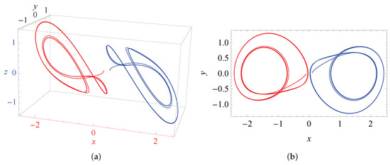
Figure 2. A symmetrical pair of orbits, in blue and red, corresponding to the symmetrical initial conditions $(0.1,0.02,0.01)$ and $(-0.1,-0.02,-0.01)$, respectively ($\mu =1.68;\omega =1;\beta =1.0;\mathrm{tmax}=200$). (a) 3D view of two symmetrical orbits. (b) The projection on the $x-y$ plane of two symmetrical orbits.

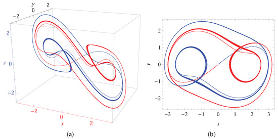
Figure 3. A symmetrical pair of orbits, in blue and red, corresponding to the initial conditions $(0.01,0.02,0.01)$ and $(-0.01,-0.02,-0.01)$, respectively ($\mu =2;\omega =0.88;\beta =1.0;\mathrm{tmax}=1000$). (a) 3D view of two symmetrical orbits. (b) The projection on the $x-y$ plane of two symmetrical orbits.

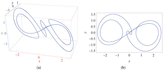
Figure 4. A symmetrical orbit relative to $O(0,0,0)$ corresponding to the initial conditions $(0.1,0.02,0.01)$ ($\mu =1.8;\omega =1;\beta =1.0;\mathrm{tmax}=200$). (a) 3D view of a symmetrical orbit. (b) The projection on the $x-y$ plane of a symmetrical orbit.

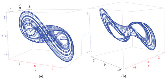
Figure 5. A strange attractor that is symmetric relative to $O(0,0,0)$ (initial conditions $(0.01,0.02,0.01)$; $\mu =2;\omega =0.9;\beta =1.0;\mathrm{tmax}=1000$). (a) 3D view of a symmetrical strange attractor. (b) The same attractor, from other angle.

6. Conclusions

In this paper, a class of jerk equations which depends on the functions V and $f_{\mu }$, namely $\left(J\right):\stackrel{⃛}{x}+\beta \ddot{x}+V^{″}\left(x\right)\dot{x}=f_{\mu }\left(x\right),\beta >0,\mu \in \mathbb{R}$ is considered. Geometric symmetries of an arbitrary jerk equation are discussed. Particularly, under some conditions fulfilled by V and $f_{\mu }$, the invariance to inversion of the above jerk equation $\left(J\right)$ is obtained. Under these conditions, stability, bifurcations, integrable deformations, and chaotic behavior of $\left(J\right)$ are investigated. More precisely, the stability of the equilibrium points of $\left(J\right)$ is discussed using the Routh–Hurwitz theorem. Furthermore, using the partial derivatives of $f_{\mu }\left(x\right)=f(x,\mu ),$ sufficient conditions for $\left(J\right)$ to display codim 1 bifurcations are presented. These results are used to study a particular jerk equation which has a double-fork symmetrical bifurcation diagram of equilibrium points. Moreover, the local center manifold theory is applied to study the stability in the case of zero real part of the eigenvalues of the corresponding Jacobian matrix. Then, integrable deformations of $\left(J\right)$ that belong to the same class of jerk equations are constructed. In addition, they are used to stabilize some equilibrium points of $\left(J\right)$. Finally, a piecewise jerk equation of type $\left(J\right)$ which has a symmetric strange attractor is introduced, and some numerical simulations are presented.

As future work, we mention the study of codim 2 bifurcations of the considered system when $\beta$ and $\mu$ are parameters. In addition, if $f_{\mu }$ is a piecewise function, the analysis of the dynamical properties of the corresponding piecewise jerk equation can be performed. In particular, multistability and hidden attractors of the proposed chaotic piecewise jerk equation can be investigated.

References

- Schot, S.H. Jerk: The time rate of change of acceleration. Am. J. Phys. 1978, 46, 1090–1094. [Google Scholar] [CrossRef]
- Sprott, J.C. Some simple chaotic jerk functions. Am. J. Phys. 1997, 65, 537–543. [Google Scholar] [CrossRef]
- Coullet, P.H.; Tresser, C.; Arnéodo, A. Transition to stochasticity for a class of forced oscillators. Phys. Lett. A 1979, 72, 268–270. [Google Scholar] [CrossRef]
- Sprott, J.C. Simple chaotic systems and circuits. Am. J. Phys. 2000, 63, 758–763. [Google Scholar] [CrossRef]
- Munmuangsaen, B.; Srisuchinwong, B.; Sprott, J.C. Generalization of the simplest autonomous chaotic system. Phys. Lett. A 2011, 375, 1445–1450. [Google Scholar] [CrossRef]
- Wei, Z.; Sprott, J.C.; Chen, H. Elementary quadratic chaotic flows with a single non-hyperbolic equilibrium. Phys. Lett. A 2015, 379, 2184–2187. [Google Scholar] [CrossRef]
- Joshi, M.; Ranjan, A. An autonomous simple chaotic jerk system with stable and unstable equilibria using reverse sine hyperbolic functions. Int. J. Bifurc. Chaos 2020, 30, 2050070. [Google Scholar] [CrossRef]
- Liu, M.; Sang, B.; Wang, N.; Ahmad, I. Chaotic dynamics by some quadratic jerk systems. Axioms 2021, 10, 227. [Google Scholar] [CrossRef]
- Lazureanu, C. On the Hamilton-Poisson realizations of the integrable deformations of the Maxwell-Bloch equations. Comptes Rendus Math. 2017, 355, 596–600. [Google Scholar] [CrossRef]
- Lazureanu, C. Hamilton-Poisson Realizations of the Integrable Deformations of the Rikitake System. Adv. Math. Phys. 2017, 27, 4596951. [Google Scholar] [CrossRef] [Green Version]
- Femat, R.; Campos-Delgado, D.U.; Martínez-Lopéz, F.J. A family of driving forces to suppress chaos in jerk equations: Laplace domain design. Chaos 2005, 15, 043102. [Google Scholar] [CrossRef] [PubMed]
- Hu, L.; Wang, C.; Zhang, S. New results for nonlinear fractional jerk equations with resonant boundary value conditions. Aims Math. 2020, 5, 5801–5812. [Google Scholar] [CrossRef]
- Ragusa, M.A. Parabolic Herz spaces and their applications. Appl. Math. Lett. 2012, 25, 1270–1273. [Google Scholar] [CrossRef] [Green Version]
- Gilmore, R.; Letellier, C. The Symmetry of Chaos; Oxford University Press: New York, NY, USA, 2007. [Google Scholar]
- Martin, G. Transformation Geometry: An Introduction to Symmetry; Springer: New York, NY, USA, 1982. [Google Scholar]
- Sprott, J.C. Simplest chaotic flows with involutional symmetries. Int. J. Bifurc. Chaos 2014, 24, 1450009. [Google Scholar] [CrossRef]
- Gantmacher, F.R. Matrix Theory; Chelsea Pub. Co.: New York, NY, USA, 2000; Volume 2. [Google Scholar]
- Lyapunov, A.M. Problème Générale de la Stabilité du Mouvement; Princeton University Press: Princeton, NJ, USA, 1949; Volume 17. [Google Scholar]
- Perko, L. Differential Equations and Dynamical Systems, 3rd ed.; Texts in Applied Mathematics 7; Springer: New York, NY, USA, 2001. [Google Scholar]
- Guckenheimer, J.; Holmes, P. Nonlinear Oscillations, Dynamical Systems, and Bifurcations of Vector Fields, Applied Mathematical Sciences; Springer: Berlin/Heidelberg, Germany, 1983. [Google Scholar]
- Kuznetsov, Y.A. Elements of Applied Bifurcation Theory; Springer: New York, NY, USA, 1998. [Google Scholar]
- Sotomayor, J. Generic bifurcations of dynamical systems. In Dynamical Systems; Peixoto, M.M., Ed.; Academic Press: New York, NY, USA, 1973; pp. 561–582. [Google Scholar]
- Osipenko, G. Center Manifolds. In Encyclopedia of Complexity and Systems Science; Meyers, R., Ed.; Springer: New York, NY, USA, 2009. [Google Scholar] [CrossRef]
- Lazureanu, C. Integrable Deformations of Three-Dimensional Chaotic Systems. Int. J. Bifurc. Chaos 2018, 28, 1850066. [Google Scholar] [CrossRef]
- Lorenz, E.N. Deterministic nonperiodic flow. J. Atmos. Sci. 1963, 20, 130–141. [Google Scholar] [CrossRef] [Green Version]
- Arneodo, A.; Coullet, P.; Tresser, C. Possible New Strange Attractors With Spiral Structure, Communications in Mathematical. Physics 1981, 79, 573–579. [Google Scholar]
- Arneodo, A.; Coullet, P.; Tresser, C. Oscillators with Chaotic Behavior: An Illustration of a Theorem by Shil’nikov. J. Stat. Phys. 1982, 27, 171–182. [Google Scholar] [CrossRef]
Publisher’s Note: MDPI stays neutral with regard to jurisdictional claims in published maps and institutional affiliations. |
© 2022 by the author. Licensee MDPI, Basel, Switzerland. This article is an open access article distributed under the terms and conditions of the Creative Commons Attribution (CC BY) license (https://creativecommons.org/licenses/by/4.0/).