Abstract
For the application of parallel robots in the grinding industry, a parallel robot equipped with a constant force actuator that produces a constant force for grinding is designed. To study the characteristics of the parallel robot’s spatial positions and poses, the inverse solutions of the moving platform’s spatial positions and poses as well as the workspace where objects were ground were established by using DH parameters and geometric methods. The experimental results showed that the workspace where objects were ground was a cylinder with a cross section similar to a symmetric circular sector. To analyze the characteristics of the forces produced by the parallel robotic system, the dynamics equation was established via the Newton–Euler method to verify the rationality of the force decoupling design. Theoretical calculation combined with simulation and experimental analyses confirmed the viability of the theoretical analyses which lay a theoretical foundation for the design, manufacture and control of the parallel robotic system proposed in this paper.
1. Introduction
Parallel robots’ mechanisms are advantageous due to their large mass–stiffness ratio, small cumulative errors, high precision and suitability for high speeds and heavy loads [1,2,3]. They are very suitable for the grinding industry. However, the development and application of parallel robots have been limited because of the easy coupling of grinding forces produced by parallel robots and complex spatial motion and control of parallel robots. In this paper, a new 5-degrees-of-freedom (5-DOF) parallel robotic grinding system is designed. The proposed 5-DOF parallel robot, combined with the constant force output actuator produced by a company in Austria called Ferrobotics, has a force decoupling design and produces a constant force to grind objects.
Many scholars have carried out some research and analyses of the characteristics of parallel robots’ positions, poses and forces. Zhao Yongsheng [4] designed a 5-UPS (Universal joint + Prismatic pair + Spherical pair)/1-PRPS (Prismatic pair + Revolute pair + Prismatic pair + Spherical pair) 5-degrees-of-freedom parallel machine tool, the constraining branch of which is in the form of PRPS (Prismatic pair + Revolute pair + Prismatic pair + Spherical pair). The structure is relatively simple and can realize the corresponding constraint functions [5]. The driving branch is in the form of the commonly used UPS (Universal joint +Prismatic pair + Spherical pair). The screw theory and DH parameters were applied to analyze the kinematics of the machine tool, and the theoretical analysis was verified with the prototype. Wu Guanglei [6] designed a series-parallel robot, introduced Cartesian stiffness matrix and stiffness matrix decoupling to optimize its structural parameters and improved the elastic static performance in the grinding process [6]; Xu Peng [7] designed a polishing series-parallel robot for machining ultra-stiff materials. With the spatial closed-loop vector method and exponential product formula, the kinematic characteristics of the series-parallel mechanism, such as positions, speeds, singularities and workspace, were analyzed respectively, and the proposed series-parallel robot is suitable for free-form-surface polishing; Tian Heqiang [8] designed a 6-DOF parallel grinding robot which is applied to surgeries and proposed different interpolation algorithms for different grinding surfaces to control the robot. Experiments verified the feasibility and accuracy of the parallel grinding robot in surgeries and summarized its innovations and limitations; Mei bin [9] proposed an elastic geometric error modeling method and weighted regularization method to eliminate the errors of parallel grinding robots. Experiments showed that the accuracy of parts processed by the abovementioned methods was significantly improved [9].
Although parallel robots have received the attention of many experts, scholars and enterprises at home and abroad, the research and application of parallel robots mostly focus on motion clamping, milling and other industries, and there is little research on its application in the grinding industry. At present, the robots employed in the grinding industry are mainly series robots. The early application of series robots in the grinding industry mainly focused on occasions where objects with simple shapes and objects with low precision requirements were created.
In recent years, European and American countries have increased investment in the robot grinding industry, and some key technologies have also been advanced. The application of series robots in the field of grinding has been gradually promoted. With their own advantages, the United States, Finland and other developed countries have successively developed commercial machines with flexible movement, good universality and high precision. At present, parallel robots are developing rapidly in milling, aircraft simulation and other industries. However, because the grinding force of parallel robots is easily combined with other forces, the grinding force perpendicular to the grinding point is affected by multiple inputs at the same time. As the spatial motion and control are complex, the domestic grinding industry still adopts more series robots with more mature technology. The development of parallel robots is relatively slow. In view of the above situation, this paper designed a new 5-DOF parallel grinding robot combined with a constant force output actuator produced by Ferrobotics, a company in Austria, to realize the force type decoupling, grinding with a constant force of the parallel robot. Since pose space control is the premise of grinding and force control is an important guarantee to realize high-precision grinding, this paper mainly analyzed the position, pose and spatial characteristics of the designed model as well as forces affecting the designed model. The virtual prototype model under the SolidWorks three-dimensional software environment was established. The optimization design was carried out and the rationality of the structural design, the correctness of the theoretical analysis and the feasibility of the practical application were proven by using the methods of theoretical analysis and simulation analysis. Finally, the physical model of the the new 5-DOF parallel grinding robot with a constant force output actuator was established for experimental analysis.
To sum up, many scholars have designed parallel robots for specific work requirements, analyzed their poses, positions and dynamics, and achieved fruitful outcomes. Nonetheless, they cannot realize constant force grinding with a force decoupling design and a constant force output actuator. This paper aims to analyze the pose, position and dynamic characteristics of the proposed parallel grinding robot so as to lay a theoretical foundation for motion control and the error analysis of the proposed parallel grinding robot.
2. Introduction of the Parallel Grinding Robot
Using driving branches and constraining branches is an important method for the construction of a parallel mechanism, which is adopted in this paper. As is shown in Figure 1, the parallel robot includes a fixed platform, a moving platform, four driving branches (UPS Universal joint + Prismatic pair + Spherical pair) and a constraining branch (RPS Revolute pair + Prismatic pair + Spherical pair). The four inclined angles of the fixed platform are connected with the moving platform through four identical driving branches (UPS), and the center of the fixed platform is connected with the center of the moving platform through a constraining branch (RPS).
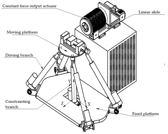
Figure 1.
The 4-UPS/1-RPS parallel grinding robot.
The parallel grinding robot drives the spatial motion of the parts to be ground, and the constant force output actuator provides the grinding force perpendicular to the grinding point. Figure 2 is the schematic diagram of the constant force output actuator, which can provide high-precision constant force output in one-dimensional direction along its axis (i.e., perpendicular to the grinding point plane). During operation, the filtered and compressed air enters the constant force output actuator from the air inlet, and the control cable is connected to the control box of the constant force output actuator. The internal sensor of the constant force output actuator converts the detected internal air pressure into output force data and transmits it to the controller. According to the real internal change in air pressure, the controller regulates the pressure and rate of the air inlet to keep the output force of the output actuator constant.
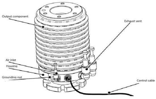
Figure 2.
Constant force output actuator.
3. Analysis of the Characteristics of the Parallel Grinding Robot’s Spatial Poses and Positions
3.1. Constrained Branch DH Analysis
The spherical pair was simplified into three one-degree-of-freedom revolute pairs whose rotation axes are perpendicular to each other. According to the coordinate system configuration principle of DH parameters, the coordinate system of the constraining branch (RPS) was established. The corresponding DH parameters are shown in Table 1.

Table 1.
Constraining branch DH parameters.
In Table 1, the variables are θ1, d2, θ3, θ4 and θ5. The constants are α2 = −90° and α3 = α4 = α5 = 90°. ls0 is the distance from the center of the fixed platform to the axis of the revolute pair in the constrained branch. According to the principle of coordinate system transformation and DH parameters, the transformation matrix of the moving platform relative to the fixed platform is described in (1).
In (1) .
If the z–y–z Euler angles are used to describe the position and pose of the moving platform relative to the fixed platform, the transformation matrix between the moving platformand the fixed platform can be demonstrated in (2).
In (2), α, β and γ are the Euler angles and , and are the coordinates of the center of the moving platform in the fixed coordinate system. With the comparison between (1) and (2), Equation (3) can be obtained.
The moving platform is a constant, that is, the z axis coordinate of the center of the moving platform is a fixed value, indicating that the parallel robot constrains are moving along the Z-axis (one-degree-of-freedom). The one degree of freedom is constrained by the combined action of the constant force output actuator and the linear slide.
3.2. Inverse Solution Analysis of the Driving Branch (UPS)
Generally, the driving branch is the input link that controls the motion of the moving platform. The constraining branch restricts one or several degrees of freedom of the moving platform. In this paper, the degree of freedom of the parallel grinding robot to be constrained is the degree of freedom that moves along the direction of the constant force output actuator. The constraining branch adopts the RPS form which includes the revolute pair, prismatic pair and spherical pair. The structure is relatively simple and can achieve the corresponding constraining function. The driving branch adopts the mature UPS form which includes the universal joint, prismatic pair and spherical pair. Such a structural design can not only achieve the decoupling of degrees of freedom, but also results in the driving branch as a driving part being mainly subject to the gravity of the moving platform, fixture and parts to be processed and the spatial motion force. The forces applied on the driving branch will not increase in corresponding multiples with the increase in grinding processing force. The constraining branch is mainly used to constrain the degrees of freedom of the parallel grinding robot along the Z-axis, and, with the constant force output actuator, together bears the grinding forces perpendicular to the grinding point during the grinding process to achieve the decoupling of different types of forces. The moving platform is a disc-shaped structure. Four spherical pairs are evenly distributed along the circumferential direction in order to avoid the strange position of the moving platform in the initial position. The four driving branches are not completely symmetrical to the center of the moving platform. The fixed platform adopts the form of a rectangle and the four universal joints are distributed in the four oblique positions of the fixed platform. As is shown in Figure 3, the fixed coordinate system S is established on the fixed platform and the moving coordinate system M is established on the moving platform. The initial directions of the two coordinate systems are consistent. When the structure sizes of the parallel robot are given, the coordinates of each hinge in the corresponding coordinate system can be obtained by using the geometric relationships.
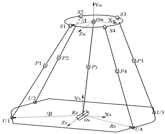
Figure 3.
The schematic diagram of the movement of the 4-UPS/1-RPS parallel grinding robot.
The four spherical pairs connected with the moving platform are evenly distributed in the circumferential direction, and therefore the coordinates of each hinge Si on the moving platform can be described by Equation (4).
The four universal joints connected with the fixed platform are distributed at the four corners of the fixed platform. The coordinates of each universal joint U on the fixed platform in the fixed coordinate system can be described by Equation (5).
The position vector from the center Om of the moving platform to the spherical pair Si is described by Equation (6).
The coordinates of the moving platform center Om in the fixed coordinate system are represented by . As per (2), Equation (7) can be obtained.
In the quadrilateral OmOsUiSi, represents the vector from OS to Si, and represents the rotation matrix of moving platform M relative to fixed platform S. According to the geometric relationships, the driving branch vector is shown by (8).
Thus, the length of the driving branch is = (= 1, 2, 3, 4). The length of each driving branch can be obtained, and the position and pose of the moving platform can be controlled by controlling the length of each driving branch.
3.3. The Analysis of the Workspace of the Parallel Grinding Robot Where Grinding Takes Place
Workspace is the working area of the robot’s manipulator. The workspace’s size is an important index to measure the performance of robot [10], and it is an important embodiment of the effectiveness and applicability of robot.
3.3.1. Influencing Factors of Workspace
The factors affecting the workspace of the parallel grinding robot include the lengths of the driving branches, the rotation angles of the kinematic pairs, the mutual interferences of the connecting links, etc. [11]. The maximum and minimum lengths of the driving branches are , respectively, and . A new sentence has been added right before Figrue 4. The new sentence includes the citation of Figure 4.
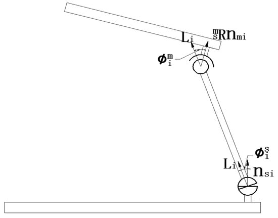
Figure 4.
The diagram of the constraining kinematic pairs.
The unit vector passing through the center Om on the moving platform and parallel to the Y-axis of the moving coordinate system is . = (0, 1, 0)T and the position vector of this unit vector in the fixed coordinate system is. The rotation angle of the i-th spherical pair along the circumferential direction on the moving platform is =. According to (2), the position vector of the constraining branch in the fixed coordinate system is =T. The rotation angle of spherical pair in the constrained branch is =. The unit vector passing through the center Os on the fixed platform parallel to the Y-axis is and =(0, 1, 0)T. The rotation angle of the i-th universal joint on the fixed platform is = . If the diameter of the driving branch is D and Di is the shortest distance between the center lines of two adjacent driving branches, the condition to avoid mutual interference between two adjacent driving branches is D ≤ Di. The limit rotation angles of the spherical pairs are and . The limit rotation angles of each universal joint are and . The limit positions of the prismatic pair in the constrained branch are , respectively. The limit rotation angles of the rotation pair in the constrained branch are . The parallel grinding robot shall meet the constraints described in Equation (9).
Equation (9) describes the constraints that should be met in the motion process of the parallel grinding robot and limits the reachable workspace and feasible solution of the parallel robot.
3.3.2. Analysis of the Spatial Characteristics of the Places Where Grinding Takes Place
Grinding is generally carried out from points to lines and to surfaces. The grinding tool is perpendicular to the place where grinding takes place. The place where grinding takes place is the main concern when grinding process is analyzed. The parallel robot system is that the grinding tool is relatively fixed, and the moving platform drives the spatial motion of the parts to be machined, so that the place where grinding takes place is perpendicular to the grinding tool to realize constant force grinding [12]. Therefore, when the workspace of the parallel robot is analyzed, the place where grinding takes place on the part to be machined corresponding to the end of the grinding tool should be taken as the research object.
The position with a distance YT along the Y-axis to the moving platform was taken as the grinding point and the research object [13]. The workspace of the parallel grinding robot is analyzed and the position vector of the grinding point in the moving coordinate system is = ()T whose position vector in the fixed coordinate system is . According to (7), the vector of the grinding point in the fixed coordinate system is shown in (10).
3.3.3. Example Calculation
Considering the actual application of the parallel grinding robot, the actual assembly size of the fixture and parts to be processed, the working process of the driving branches and the overall size of the prototype, the main structural parameters of the parallel grinding robot are shown in Table 2.
Table 2.
Structural parameters.
Due to the complexity of the motion of the parallel grinding robot, the spatial analysis of the grinding point of the parallel grinding robot is usually complex, which is generally a nonlinear expression. Some are even implicit expressions. Hence, it is difficult to obtain the numerical solution directly. In this paper, the brute-force search was used to draw the three-dimensional graphs of grinding points. Equation (9) is the constraint condition and the grinding points of (10) are the objective function. The exhaustive method was applied in MATLAB to obtain the three-dimensional scattered-points set meeting the constraint condition, as is shown in Figure 5. All the outermost points in the three-dimensional scattered-points set were taken to form a new set, and then the envelope surface of the gap (inexhaustible points) between adjacent points in the new set is drawn by surface approximation so as to obtain the grinding point workspace of the parallel grinding robot to prevent the dead zone that the parallel robot may not reach when performing tasks, as is shown in Figure 6 and Figure 7.
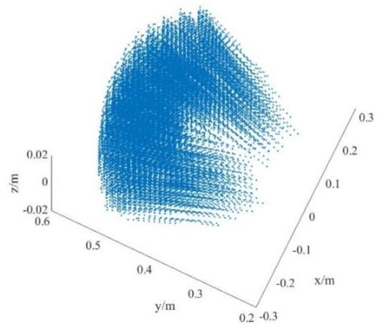
Figure 5.
Three-dimensional scatter-points diagram.
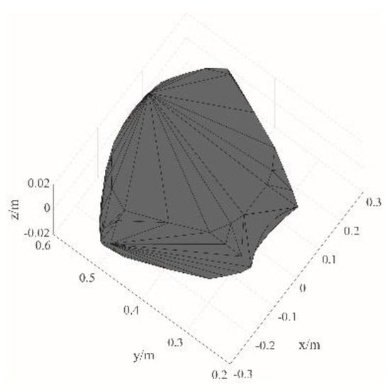
Figure 6.
Three-dimensional diagram of workspace.
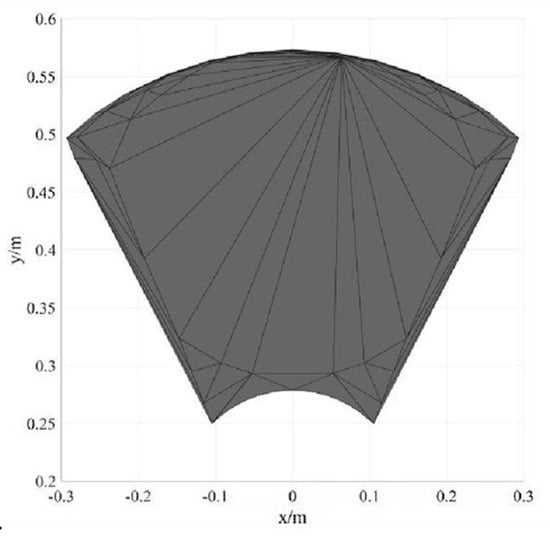
Figure 7.
X–Y plane of workspace.
According to the analysis results of MATLAB and the system structure, the grinding point workspace of the parallel grinding robot is a cylinder with a cross section similar to a circular sector. In the cross section, the ranges of the grinding strokes in the X direction and Y direction are about −0.3 m to 0.3 m and 0.25 m to 0.57 m, respectively. The upper and lower ends are arc surfaces, and the lower end is gradually reduced to −0.11 m–0.11 m. This workspace meets the common constant force grinding applications.
4. Dynamic Modeling and Force Decoupling Analysis
4.1. Kinematic Analysis of the Constraining Branch
The spherical pair with three degrees of freedom in the constraining branch RPS is equivalent to three revolute pairs, each of which has one degree of freedom. The position and pose of the moving platform relative to the fixed platform can be expressed as = []T. are the coordinates of the center of the moving platform . In the fixed coordinate system. represents the attitude Euler angle of the moving platform in the fixed coordinate system. The constraining branch can be expressed as = [,,,,]T.
From the derivatives of both sides of 43, the relationship between DH parameters of the constraining branch and pose parameters of the moving platform is obtained, and it is described in Equation (11).
In Equation (11), = []T and = [, , , , ]T.
is the velocity mapping matrix between the constraining branch and the moving platform (i.e., the first-order influence coefficient matrix).
From the derivatives of both sides of Equations (11) and (12), the following can be obtained.
In Equation (12), = []T and = [, , , , ]T.
is the acceleration mapping matrix between the constraining branch and the moving platform (i.e., the second-order influence coefficient matrix).
The relationship between the pose parameters of the moving platform and the constraining branch parameters is obtained when both sides of Equations (11) and (12) are multiplied by []−1.
The constraining branch is composed of a revolute pair, a prismatic pair and a spherical pair. Its main rotational inertia and the forces that affect it are concentrated on the cylinder block and linear moving link of the prismatic pair. The revolute pair and spherical pair are ignored in the dynamic analysis. The coordinate system 1 where the revolute pair axis is located was chosen as the reference coordinate system. The schematic diagram of linear velocity and angular velocity of the constraining branch’s cylinder block is shown in Figure 8, and the relationship between them and constraining branch velocity parameters is shown in Equation (15)
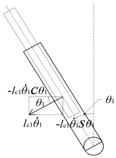
Figure 8.
The schematic diagram of cylinder block speed of constraining branch.
Similarly, coordinate system 1 was chosen as the reference coordinate system, the schematic diagram of linear velocity and angular velocity of the constraining branch’s linear moving link are shown in Figure 9. The relationship between them and the constraining branch velocity parameters is described in Equation (16).
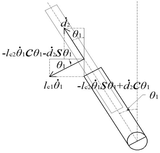
Figure 9.
The schematic diagram of constraining branch push rod speed.
According to the coordinate transformation in Section 2, in the fixed coordinate system, the relationship between the velocity DH parameters of the constraining branch and the cylinder block and linear moving link can be expressed in Equation (17).
Equation (13) was inserted into Equations (17) and (18) to obtain the conversion relationships between the velocities and angular velocities of the constraining branch’s cylinder block and linear moving link and the moving platform’s pose and velocity parameters in the fixed coordinate system. The relationships are described in Equations (19) and (20).
4.2. Motion Analysis of the Driving Branch Components
As is shown in Figure 10, is the linear velocity of the moving platform’s center point Bo and is the angular velocity of the moving platform. The velocity of the center point of the spherical pair is and is the unit direction vector of the driving branch
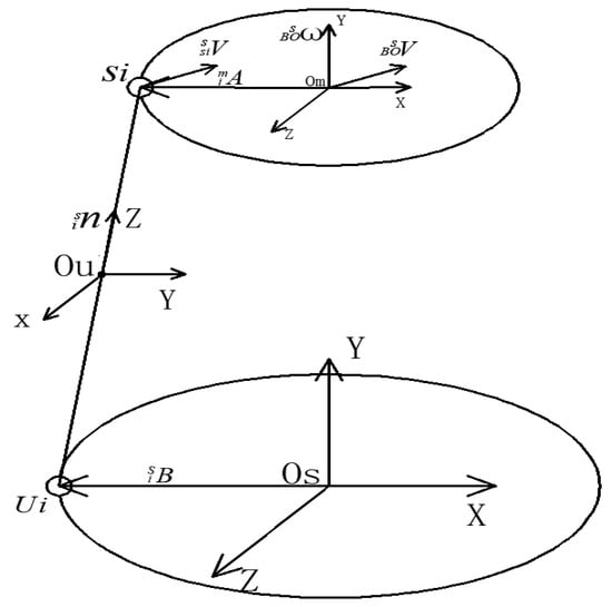
Figure 10.
Schematic diagram of the driving branch’s speed.
The motion of the moving platform was the research object. The velocity of the center of the i-th spherical pair is shown in Equation (21).
When the driving branch was taken as the research object, the velocity of the center of the i-th spherical pair could be expressed in Equation (22).
In Equations (21) and (22), represents the angular velocity of the driving branch in the fixed coordinate system, and represents the linear velocity of the driving branch.
As and , both sides of Equation (22) are multiplied by at the same time, the scalar product of which is shown in Equation (23).
Equation (21) is inserted into Equation (23) to obtain Equation (24).
In Equation (24), is the anti-symmetric matrix of . Both sides of Equation (24) are multiplied by simultaneously to obtain Equation (25).
Equation (21) is inserted in Equation (25) to obtain the expression of angular velocity of the driving branch in the fixed coordinate system.
The derivatives of both sides of Equation (24) are the linear acceleration of the driving branch .
In Equation (27), I is the third-order identity matrix. The angular acceleration of the driving branch is the derivatives of both sides of Equation (25).
The distance from the center of mass of the cylinder block to the center of the universal joint is and the distance from the center of mass of the linear moving link to the center of the spherical pair is . According to the velocity analysis method of theoretical mechanics, in the fixed coordinate system, the centroid velocity and centroid acceleration of the driving branch’s cylinder block are described in Equations (29) and (30), respectively.
In the fixed coordinate system, the centroid velocity and centroid acceleration of the driving branch’s linear moving link are described in Equations (31) and (32), respectively.
After simplification, the speed conversion relationship between the moving platform and the driving branch’s cylinder block and linear moving link is described in Equation (33).
In Equation (33), represents the velocity matrix between the moving platform and the cylinder block of the driving branch in the fixed coordinate system.
In Equation (34), represents the velocity matrix between the moving platform and the linear moving link of the driving branch in the fixed coordinate system.
4.3. Analysis of the Mapping Relationship between the Input Velocity of the Stressed Component and the Driving Branch
According to Equation (24), in the fixed coordinate system, the input speed of the driving branch is described in Equation (36).
With =, Equation (37) can be obtained.
The analysis shows that JA is a 4 × 6 matrix, and hence Equation (38) cannot be directly inversed. The relationship matrix in Equation (38) is transformed into an n-th square matrix, which is shown in Equation (39).
Equation (39) is inserted into Equation (37) to obtain Equation (40).
In Equation (40), = and is the inverse matrix of . Equation (40) is inserted into Equation (39) with == to obtain (41).
Equation (40) is inserted into Equations (19) and (20) to obtain Equations (42) and (43).
In Equations (42) and (43), and are the mapping matrices from the input speed of the driving branch to the cylinder block and the linear moving link of the constraining branch, respectively. Equation (41) is inserted into Equation (34) to obtain Equation (44).
Equation (41) is inserted into Equation (35) to obtain (45).
In Equations (44) and (45), and are the speed mapping matrixes from the input speed of the driving branch to the driving branch’s cylinder block and the linear moving link, respectively.
4.4. Stress Analysis and Model Establishment
4.4.1. Force Analysis
The forces that affected the moving platform mainly include the inertia force, inertia moment, gravity and grinding force, as well as grinding torque during grinding.
If the fixture on the moving platform and the moving platform are simplified as a whole, the inertia force of the moving platform is shown in Equation (46).
In Equation (46), is the mass of the simplified moving platform.
The inertia moment of the simplified moving platform is shown in (47).
In (47), is the moment of inertia of the simplified moving platform.
The gravity of the simplified moving platform is shown in (48).
In the fixed coordinate system, the force and torque affecting the moving platform during grinding are shown in (49) and (50), respectively.
In (49) and (50), . are the external force and external torque affecting the moving platform, respectively.
The force on the constraining branch is mainly concentrated on the cylinder block and linear moving link, and the inertial force that affected the constraining branch is described in (51).
In (51), is the mass of the simplified constraining branch’s cylinder block and linear moving link. The inertia moment of the constraining branch’s cylinder block and linear moving link is shown in (52).
In (52), is the moment of inertia of the constraining branch’s cylinder block and linear moving link after simplification.
After simplification, the gravity of constraining branch’s cylinder block and linear moving link is shown in (53).
The coordinate system was established, as is shown in Figure 9, where is the unit position vector of the i-th universal joint under the fixed coordinate system, and the rotation matrix of the coordinate system at the centroid of the driving branch’s cylinder block and linear moving link relative to the fixed coordinate system is shown in (54).
The inertia force of the cylinder block and the linear moving link is shown in (55) and (56), respectively.
In (55) and (56), and are the masses of the driving branch’s cylinder body and linear moving link, respectively.
The torques applied on the cylinder block and linear moving link are described in (57) and (58), respectively.
In (57) and (58), and are the rational inertias of the driving branch’s cylinder block and linear moving link under the coordinate system i. The gravity of cylinder block and linear moving link are described in (59) and (60), respectively.
4.4.2. Dynamics Model of the Parallel Grinding Robot
The forces that affect the moving platform, each component of the driving branches and each component of the constraining branch needed to be mapped to the equivalent input forces of the four driving branches. The mapping matrix between the actual forces that affected each component of the parallel grinding robot and the equivalent input forces of the driving branches is the transposition matrix of the parallel grinding robot’s velocity matrix [14]. Therefore, the equivalent input force of each driving branch is as follows.
In the fixed coordinate system, the equivalent input forces mapped from the actual force affecting the simplified moving platform to the driving branches are described in (61).
In the fixed coordinate system, the equivalent input forces mapped from the actual forces affecting the cylinder block and linear moving link of the constraining branch to the driving branches are described in (62) and (63), respectively.
In the fixed coordinate system, the equivalent input forces mapped to the driving branches from the forces affecting the cylinder blocks and the linear moving links of the driving branches are described in (64).
According to the D’Alembert principle, the driving forces of the driving branches are balanced by the equivalent input forces. With , Equation (65) can be obtained.
With the known structural parameters of the parallel grinding robot and (53), the explicit relationship between the force affecting the moving platform and the driving force of the driving branch can be obtained.
4.5. Decoupling Analysis of Human Types of Parallel Machines
Whether the theoretical analysis was reasonable needed to be verified by simulation analysis. With the help of ADAMS, a virtual prototype analysis software, the kinematics simulation of the model was carried out. Given different two-point motion forms of the moving platform, the simulation curves of driving branch speed and acceleration were obtained, and the numerical solutions obtained by MATLAB were compared and analyzed.
In the structural design of the parallel grinding robot, the forces applied vertically on the grinding point and applied on the moving platform were decoupled. Whether the model design could achieve the expected goal could be verified by actual model calculation or simulation. The parameters of the virtual prototype model of the parallel grinding robot were employed in the dynamics equation, and the theoretical calculation was carried out, combined with the actual working conditions [15]. These are the main structural parameters and characteristics of the parallel grinding robot in Table 3.
Table 3.
Structural Parameters or Characteristics.
Hypothesis 1 was that the parallel grinding robot was only subjected to gravity without other external forces. The motion equation is as follows:
According to (66)–(68), the MATLAB numerical solution curve and Adam simulation solution curve of velocity and acceleration of the driving branches are shown in the Figure 11, Figure 12, Figure 13 and Figure 14.
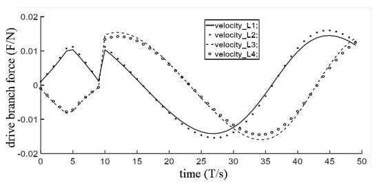
Figure 11.
Numerical solution velocity curve of the driving branches.
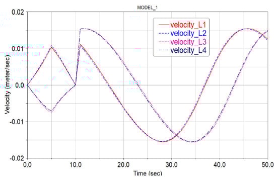
Figure 12.
Velocity curve of driving branch simulation solution.
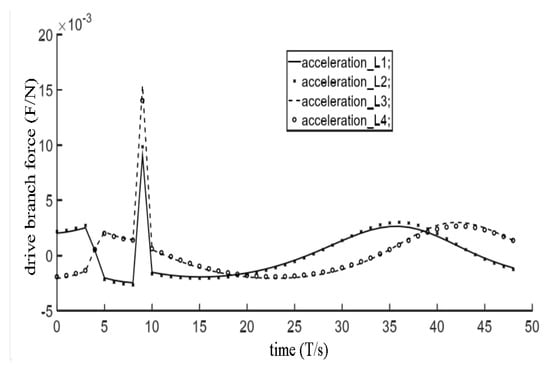
Figure 13.
Driving branch numerical solution acceleration curve.
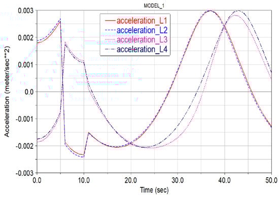
Figure 14.
Acceleration curve of driving branch simulation solution.
The other external forces on the moving platform were . The external moment was 0. The numerical solution was calculated with MATLAB, and the stress diagrams of four driving branches were obtained, as is shown in Figure 15. The analysis showed that in the linear motion stage, the forces on the driving branch L1 and the driving branch L4 decreased smoothly, and the forces on the driving branch L2 and the driving branch L3 increased smoothly. The force curves of the driving branch L1 and the driving branch L4 changed similarly and had different sizes, and the driving branch L2 and the driving branch L3 changed similarly and had different sizes. This result was consistent with the symmetrical structure design of the parallel grinding robot. In the circular motion stage, the forces on the four driving branches changed in sine and cosine waves and also met the qualitative law in the linear motion stage, which was consistent with the spatial motion. During the entire movement, the forces on the four driving branches were uniform. The minimum forces on L1 and L2 were 6 N near the 26th second, and the minimum forces on L3 and L4 were 6 N near the 15th second. The maximum forces on the four driving branches appeared near the 40th second, which was about 17.5 N, but the forces on the four driving branches changed slightly near the 10th second, that is, in the moment connecting the linear motion and circular motion, the forces affect the parallel grinding robot suddenly changed. This corresponded to the sudden change in acceleration in acceleration analysis. In the later trajectory planning and grinding process, the impact should be reduced.
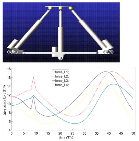
Figure 15.
Numerical solution curves under gravity only.
Whether the theoretical analysis was correct or not needed to be verified by simulation or experiment, and the virtual prototype model was imported into ADAMS simulation analysis software. The virtual prototype model was imported into Adams and the spatial drive was applied to the moving platform to make the moving platform move when only affected by gravity, according to the motion equations of hypothesis 1. The force simulation solution of the driving branch is shown in Figure 16.
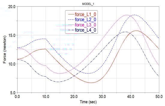
Figure 16.
Simulation solution curves under gravity only.
Through the comparative analysis, the force curves of the numerical solution and the simulation solution were basically identical. In the linear motion stage, the forces on the driving branch L1 and the driving branch L4 gradually decreased, and the forces on the driving branch L2 and the driving branch L3 gradually increased. In the circular motion stage, the forces also changed in sine and cosine waves. The result was the same as the MATLAB numerical solution and, therefore, the rationality of the model solution and analysis was verified [16]. However, the overall force of the numerical solution was smaller than that of the simulation analysis. Considering the establishment process of the mathematical model, in the theoretical analysis the forces affecting the constraining branch are simplified as the forces affecting the cylinder block and linear moving link. The revolute pair and spherical pair had small inertia forces and rotational inertias which were ignored. Similar simplification was also made in the force analysis of the driving branches. In the force analysis of the moving platform, the overall dimensions of the fixture were ignored. The fixture and moving platform were simplified into two different disks with the same masses and rotational inertias as that of the fixture and moving platform, respectively. In the simulation analysis, only the moving platform and fixture were simplified, and the forces affecting the kinematic pairs of the constraining branch and the driving branch were not simplified. The abovementioned simplification process reduced the complexity of the whole model analysis and reduced calculation. The abovementioned simplification process created some approximation errors between the experimental results and the simulation analysis results but did not affect the correctness and rationality of the mathematical model.
Since the output force of the constant force output actuator remained unchanged in the grinding process, the external force affecting the moving platform could be simplified as a constant force along the Z-axis, and the torque of that external force is always 0.
Hypothesis 2 was that, in the grinding process, the constant force output actuator applied a constant force of 30 N to the moving platform of the parallel grinding robot, that is. The moving platform moved in the positive direction of Y-axis with an acceleration of 2 mm/s2 for 10 s. The moving platform uniformly accelerated in the first 5 S and uniformly decelerated in the next 5 S. The moving platform remained horizontal all the time, that is, the rotation angle of the moving platform was α = β = γ = 0 and angular velocity was . Angular acceleration, and the numerical curve and simulation curves of driving forces of driving branches under hypothetical 2 are shown in Figure 17 and Figure 18. Hypothesis 3 was that, in the grinding process, the constant force output actuator applied a constant force of 50 N to the moving platform of the parallel grinding robot. That is, . The motion of the moving platform in hypothesis 1 was the same as the motion of the moving platform in hypothesis 2. The numerical curve and simulation curve of the driving forces of the driving branches are shown in Figure 19 and Figure 20.
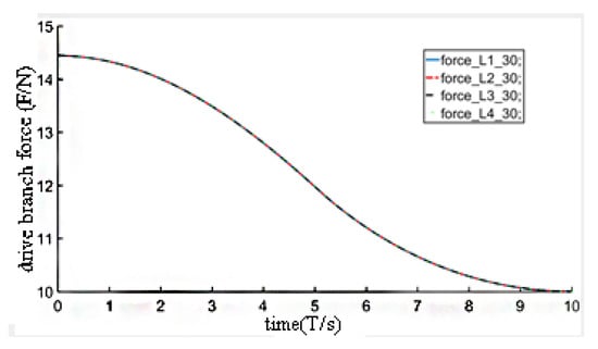
Figure 17.
Numerical curves of driving forces when .
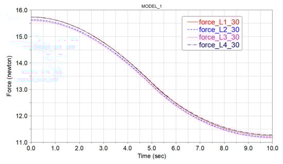
Figure 18.
Driving force simulation curves when .
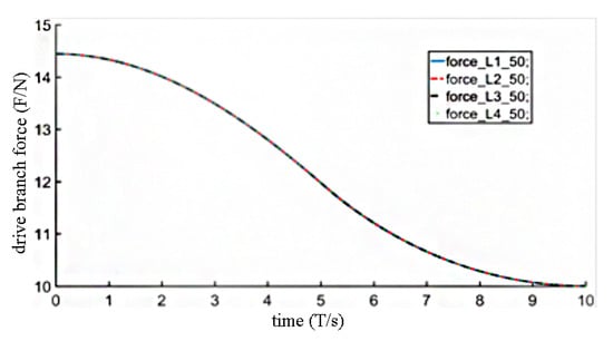
Figure 19.
Numerical curves of driving forces when .
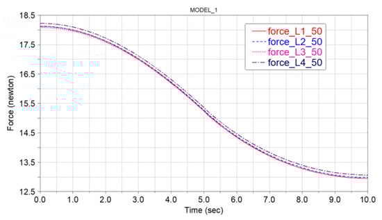
Figure 20.
Driving force simulation curves when .
After Figure 17, Figure 18, Figure 19 and Figure 20 were compared, the forces on the four driving branches changed uniformly. The numerical solution curves were the same and the force curves of the simulation solution were the same. The magnitude of the forces was similar. The forces on the four driving branches did not have a multifold increase as the external force increased. The forces on the four driving branches only increased slightly by about 2 N. The results showed that the grinding force applied by the constant force output actuator was not mainly withstood by the driving branches but by the constraining branch. The driving branches mainly bore the gravity of the moving platform, fixture and parts to be processed, and were mainly used to drive the spatial motion of parts. Similarly, the abovementioned results could be confirmed by comparing the force curves in the linear motion stage, which are shown in Figure 11 with Figure 14 and Figure 15. The forces affecting the driving branches did not increase by a corresponding multiple with the increase in the output force of the constant force output actuator, but also slightly increased by 3 N to 4 N. The abovementioned results showed that the grinding force of the parallel grinding robot’s grinding system was mainly provided by the constant force output actuator and the constraining branch. The driving forces of the parallel robot were mainly employed to drive the spatial motion of the moving platform, that is, the force decoupling in the system structure design is reasonable and feasible.
5. Experiments and Results
Experiments and Results
In the analysis of the characteristics of the spatial poses of positions of the parallel grinding robot in Section 2, the scattered-points diagram, three-dimensional diagram and cross section diagram of grinding point workspace were drawn by MATLAB. In Section 5, the independently designed grinding system was employed to verify the spatial cross section diagram of the grinding point workspace in Section 2.
As is shown in Figure 21, a pencil was installed on the moving platform of the parallel grinding robot and the grinding point trajectory was projected on a piece of white paper. The moving platform was driven to move along the maximum reachable space of its X–Y plane, as is shown in Figure 22. The cross section view of the workspace of the 5-DOF parallel grinding robot was obtained, as is shown in Figure 23.
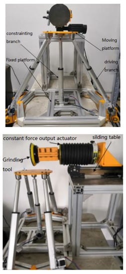
Figure 21.
The physical diagram of parallel robot grinding system.
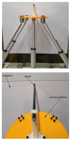
Figure 22.
The grinding point trajectory.
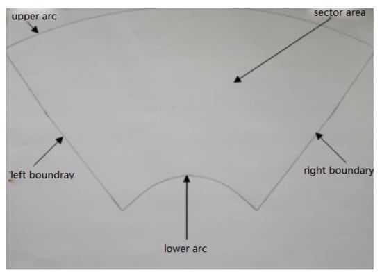
Figure 23.
Cross section of workspace.
Figure 7 was compared with Figure 23. The comparison showed that the cross section of the workspace of the grinding point obtained through the theoretical analysis was consistent with the shape of the workspace boundary curve obtained through the physical model, indicating the correctness of the theoretical analysis of the pose and position characteristics. As per Figure 23, the cross section of the workspace of the parallel robot’s grinding system model is a circular sector. The upper end of the sector is an arc with a radius of about 0.55 m and the lower end is an arc with a radius of about 0.22 m. The distance between the upper and lower arcs is about 0.32 m, and the distance between the left and right sides is about 0.58 m.
At the same time, as per the contour of the trajectory diagram, the parallel robot’s grinding system can realize accurate spatial motion, but the motion accuracy cannot be brought into full play. The analysis of the approximation errors shows that the physical model is the first prototype model. Some aspects of the dimension design and coordination are unreasonable. The fixed platform is made of aluminum. The moving platform and the universal joints were 3D printed and, therefore, the accuracy does not meet the design requirements, resulting in the low motion accuracy of the whole system.
6. Conclusions
A parallel robotic system suitable for the constant force grinding industry is proposed and the poses, positions and the force decoupling of the 4-UPS/RPS parallel grinding robot were studied by using the methods of theoretical and simulation analyses as well as experimental verifications. The main conclusions are as follows.
The inverse kinematics equation of the 4-UPS/RPS parallel grinding robot was established by using DH parameters and geometric methods. The influencing factors of the workspace were considered as constraints. The scattered-points diagram, three-dimensional diagram and cross section diagram of grinding point workspace were drawn. The results showed that the grinding point workspace was a cylinder with a cross section similar to a circular sector. The travel range in the X direction is about −0.3 m–0.3 m and the travel range in the Y direction is about 0.25 m–0.57 m. The upper and lower ends are arc surfaces. The cross section of the workspace was taken as an example. The correctness and rationality of pose, position and workspace analyses were verified by physical model experiments.
The dynamics equations of the 4-UPS/1-RPS parallel grinding robot were established by the Newton Euler method. Through calculation and simulation, when the external grinding force of the parallel grinding robot increased in multiples, the forces affecting the driving branches did not increase in multiples, indicating that there was no coupling between the grinding force perpendicular to the grinding point and the forces driving the spatial motion of parts in the grinding process. The feasibility and rationality of the force decoupling design of the 4-UPS/1-RPS parallel grinding robot were verified.
Author Contributions
Conceptualization, H.Z. and F.L.; methodology, H.Z.; software, F.L.; validation, J.W., H.Z. and F.L.; formal analysis, M.Y.; investigation, M.Y.; resources, Q.W.; data curation, Q.W.; writing—original draft preparation, H.Z. and F.L.; writing—M.Y., editing, M.Y. and F.L.; visualization, F.L.; supervision, J.W. and Q.W.; project administration, J.W. and Q.W.; funding acquisition, Q.W. All authors have read and agreed to the published version of the manuscript.
Funding
This research was funded by National Natural Science Foundation of China 51975190 and the APC was funded by J.W.
Institutional Review Board Statement
Not applicable.
Informed Consent Statement
Not applicable.
Data Availability Statement
The study did not report any data.
Conflicts of Interest
The authors declare no conflict of interest.
References
- Gosselin, C.; Schreiber, L.-T. Kinematically Redundant Spatial Parallel Mechanisms for Singularity Avoidance and Large Orientational Workspace. IEEE Trans. Robot. 2016, 32, 286–300. [Google Scholar] [CrossRef]
- Cui, Z.; Tang, X.; Hou, S.; Sun, H.; Wang, D. Calculation and Analysis of Constant Stiffness Space for Redundant Cable-Driven Parallel Robots. IEEE Access 2019, 7, 75407–75419. [Google Scholar] [CrossRef]
- Nabavi, S.N.; Akbarzadeh, A.; Enferadi, J. A Study on Kinematics and Workspace Determination of a General 6- P US Robot. J. Intell. Robot. Syst. 2018, 91, 351–362. [Google Scholar] [CrossRef]
- Qinchuan, Z.Y.Z.K.L.; Xiaojing, T. Kinematics analysis of 5-UPS/PRPU 5-DOF parallel machine tool. Chin. J. Mech. Eng. 2004, 40, 12–16. [Google Scholar]
- Wu, G. Optimal structural design of a Biglide parallel drill grinder. Int. J. Adv. Manuf. Technol. 2017, 90, 2979–2990. [Google Scholar] [CrossRef]
- Xu, P.; Cheung, C.F.; Li, B.; Ho, L.-T.; Zhang, J.-F. Kinematics analysis of a hybrid manipulator for computer controlled ultra-precision freeform polishing. Robot. Comput. Integr. Manuf. 2017, 44, 44–56. [Google Scholar] [CrossRef]
- Tian, H.; Wang, C.; Dang, X.; Sun, L. A 6-DOF parallel bone-grinding robot for cervical disc replacement surgery. Med. Biol. Eng. Comput. 2017, 55, 2107–2121. [Google Scholar] [CrossRef] [PubMed]
- Mei, B.; Xie, F.; Liu, X.J.; Yang, C. Elasto-geometrical error modeling and compensation of a five-axis parallel machining robot. Precis. Eng. 2021, 69, 48–61. [Google Scholar] [CrossRef]
- Huang, Z.; Zhao, Y.; Zhao, T. Higher Space Institutional Science; Higher Education Press: Beijing, China, 2006; pp. 89–166. [Google Scholar]
- Zhang, W.; Bai, X.; Xu, Z. Study on experimental method of end effector pose setting for indexing mechanism of space station. Mach. Des. 2018, 35, 89–94. [Google Scholar]
- Dou, Y.; Yao, J.; Gao, S.; Han, X.; Liu, X.; Zhao, Y. Dynamic modeling and driving force coordinated distribution of redundant drive parallel robots. Trans. Chin. Soc. Agric. Mach. 2014, 45, 293–300. [Google Scholar]
- Lin, W.; Li, B.; Yang, X.; Zhang, D. Modelling and Control of inverse Dynamics for a 5-DOF Parallel Kinematic Polishing Machine. Int. J. Adv. Robot. Syst. 2013, 10, 314. [Google Scholar] [CrossRef]
- Kanaan, D.; Wenger, P.; Chablat, D. Kinematic Analysis of a Serial-Parallel Machine Tool: The Verne Machine. Mech. Mach. Theory 2009, 44, 487–498. [Google Scholar] [CrossRef] [Green Version]
- Zhang, J.; Zhao, Y.; Jin, Y. Kinetostatic-Model-Based Stiffness Analysis of Exechon PKM. Robot. Comput. Integr. Manuf. 2016, 37, 208–220. [Google Scholar] [CrossRef] [Green Version]
- Cheng, G.; Xu, P.; Yang, D.; Liu, H. Stiffness Analysis of a 3CPS Parallel Manipulator for Mirror Active Adjusting Platform in Segmented Telescope. Robot. Comput. Integr. Manuf. 2013, 29, 302–311. [Google Scholar] [CrossRef]
- Xiao, S.; Li, Y.; Meng, Q. Mobility Analysis of a 3-PUU Flexure-Based Manipulator Based on Screw Theory and Compliance Matrix Method. Int. J. Precis. Eng. Manuf. 2013, 14, 1345–1353. [Google Scholar] [CrossRef]
Publisher’s Note: MDPI stays neutral with regard to jurisdictional claims in published maps and institutional affiliations. |
© 2022 by the authors. Licensee MDPI, Basel, Switzerland. This article is an open access article distributed under the terms and conditions of the Creative Commons Attribution (CC BY) license (https://creativecommons.org/licenses/by/4.0/).