Abstract
In the field of financial risk measurement, Asymmetric Laplace (AL) laws are used. The assumption of normalcy is used in traditional approaches for calculating financial risk. Asymmetric Laplace distribution, on the other hand, reveals the properties of empirical financial data sets much better than the normal model by leptokurtosis and skewness. According to recent financial data research, the regularity assumption is frequently broken. As a result, Asymmetric Laplace laws offer a simple, creative, and useful option to normal distributions when it comes to modeling financial data. We here engage AL distribution to explore specific formulas for the two commonly used risk measures, Value-at-Risk (VaR) and Conditional Value-at-Risk (CVaR). The currency exchange rates data are used to and worked out to illustrate the proposed methodologies.
1. Introduction
1.1. Literature Review on VaR and CVaR
In agriculture around the world, market risk is a major cause of revenue volatility. This necessitates the development of metrics that demonstrate agricultural risk exposure and the impact of risk mitigation measures [1]. The impact of financial data such as currency exchange rate has been extensively measured with different variables, involving GDP growth, export, and industrial production [2], even including energy consumption [3].
Financial risk is divided into three categories: market risk, credit risk, and operational risk. Market risk is described as the uncertainty that arises from fluctuations in the prices of financial assets such as interest rates, foreign exchange rates, stock prices, and commodity prices. The losses connected with an obligor’s default (or credit downgrade) are referred to as credit risk; operational risk is referred to as operational failures. In the field of financial risk management, one of the valid methods for doing such a thing is the Vaule-at-Risk (VaR) [4]. VaR was first introduced by Roy in Reference [5], and it has evolved into one of the most important risk indicators in today’s financial risk management [6]. It calculates the maximum loss in portfolio value that could occur owing to risky market factors during a particular time period at a given confidence level.
It has long been recognized how important it is to assess the risk of financial assets. Value-at-Risk has been universally used by commercial banks, asset management firms, and regulators since the 1990s. This strategy was discussed in the context of VaR, which measures the maximum loss of portfolio value that will occur over a given period at a given confidence level due to a risky market factors. The Basel Accord, for example, uses VaR to assess commercial banks’ market risk exposure. The Basel Committee on Banking Supervision (BCBS) established the worldwide capital adequacy criteria well-known as the Basel Accord. The Basel Accord was amended in 1996 to include risk-based capital to the capital requirements for market risk in the trading book. Banks must put up their own VaR models to calculate their minimum regulatory capital for market risk under the supervision of the Basel Committee. The Securities and Exchange Commission (SEC) of the United States began mandating financial institutions to report Value-at-Risk as a key indicator of market risk exposure in 1997 [7].
Financial institutions and asset managers both employ the notion of Value-at-Risk. Value-at-Risk is used to determine position limits for traders in asset management organizations; in commercial banks, Value-at-Risk is used to quantify the market risk exposure of their assets and is utilized in capital allocation [8,9].
This measure is defined as follows:
Definition 1.
Given a confidence level , the Value-at-Risk of the portfolio at the confidence level α is given by smallest number x such that the probability that the loss Y exceeds x is at most . Mathematically, if Y is the loss of portfolio, then the is the upper level α-, i.e.,
Denote
The left equation is a definition of VaR. The right equation assumes an underlying probability distribution, which makes it true only for parametric VaR. The profit of the portfolio’s diagram is the left tail with the lower level -.
Although Value-at-Risk (VaR) is commonly used to assess the risk of a risky asset or a specific portfolio losing value, its limits are becoming increasingly apparent. VaR has a fundamental flaw in that it is not a coherent measure, that is, it is not sub-additive. This indicates that a diversified portfolio may raise risk by preventing the VaR of various risk components from being added together [10]. Furthermore, VaR provides no additional details on the loss [11].
Conditional Value-at-Risk (CVaR) is an alternative risk measure to VaR that potentially addresses some of VAR’s shortcomings. The term of CVaR is derived from Rochafellar and Uryasev (2000) [12], which is also called “expected shortfall” [10], and “tail-conditional expectation” [13] simultaneously.
The CVaR is defined as the weighted average of the VaR and losses beyond the VaR, which equals the expected loss in the particular case of continuous random variables if the loss is larger than or equal to the VaR [14]. If Y denotes a portfolio’s loss, the CVaR of Y at probability level is the mean of the random variable obtained by truncating Y at and removing the lower tail. To put it another way, it is mean of the - distribution of Y. The CVaR serves as an upper bound on the value of VaR. The following is the definition of this measure:
Definition 2.
Given a confidence level , let Y be the loss of a portfolio at some future time; then, we define conditional value-at-risk (CVaR) as
An equivalent definition of CVaR in terms of the quantile function of Y is
CVaR can also be defined as the average VaR for small tail probabilities, i.e.,
For standard normal distribution, we have
where , which is the probability density function of the standard normal distribution. is the quantile of standard normal distribution.
Consequently, the CVaR for a normal distribution is
Let denote the corresponding order statistics from a random sample . The nonparametric estimate of CVaR is the corresponding empirical tail mean,
where denotes either of the two integers closest to .
1.2. Research Approaches of VaR
In financial mathematics and financial risk management, a finance firm may need to calculate the potential losses in value of a risky asset or specific portfolio over a defined period for a given confidence level. Assume we are looking for huge losses in a certain portfolio, more specifically, losses that are unlikely to occur more than once every hundred consecutive days. We claim we are looking for a daily value at risk and a 99% confidence level. Except for potential losses, potential profits also can be computed by VaR through equal to 99%.
For instance, a corporation might report a daily value at risk of $2 million with a 99% confidence level. This remark indicates that the corporation believes there is a less than 1% possibility that it will lose $2 million the next day. A high VaR for an investing firm indicates that the firm’s investments are overly hazardous, and there should be a structural adjustment [15].
To calculate VaR, first identify market elements that affect the portfolio’s value, such as interest rates, exchange rates, and share prices. In general, VaR is derived by first modeling a portfolio’s total return distribution. The result at the percentile corresponding to the appropriate confidence level is then calculated. The common methodologies to VaR could be investigated in three streams: parametric methods based on a volatility models, nonparametric approaches based on the historical simulation, and Monte Carlo simulation.
1.2.1. Parametric Method
When it comes to hedge fund managers, the parametric approach VaR (also known as Variance–Covariance VaR) calculation is the most commonly utilized method of calculation in practice. The financial data are assumed to be distributed in the case of parametric approaches. Under parametric approaches, the VaR at confidence level is just the quantile of the distribution at the confidence level.
The most important assumption made by managers who use parametric VaR is that their portfolio returns are normally distributed. This method is popular, since the mean and standard deviation of the portfolio are the only variables that must be calculated.
An example of a parametric VaR calculation is as follows:
Mean ($ terms): $64,000
Standard Deviation ($ terms): $80,000
Z-Score for 95% Confidence: 1.65
Standard Deviation ($ terms): $80,000
Z-Score for 95% Confidence: 1.65
Calculated VaR for the period with 95% Confidence is:
64,000 − 80,000 (1.65) = −$68,000
The brevity of the calculations and the ease with which the data for the inputs may be acquired are two of this method’s strengths, as seen above. The assumption of normality is the method’s major flaw. In fact, there are evident deviations from the norm in financial data. The majority of financial data are generally skewed and heavy tailed. Another issue with parametric methods is that they are ineffective when the portfolio has discontinuous payoffs.
1.2.2. Nonparametric Methods
To estimate VaR, nonparametric approaches use empirical quantiles of the data. Nonparametric estimate is a straightforward method that makes few assumptions about the underlying financial data’s statistical distributions. As a result, it is flexible enough to deal with data with heavy tails. We just need to rank all of the past historical returns in terms of lowest to highest and compute with a predetermined confidence rate what the lowest return historically has been.
Consider a random sample , let denote the corresponding order statistics from this random sample; then, the nonparametric estimate of VaR is the empirical quantile,
where denotes either of the two integers closest to .
Nonparametric estimation is based on previously collected data. Nonparametric estimates will underestimate or overstate VaR if there is a permanent shift in significant market drivers, such as regulatory changes.
1.2.3. Monte Carlo Simulation
Monte Carlo simulation is comparable to Historical Simulation in that it estimates VaR by simulating risk factor situations and revaluing all holdings in a portfolio for each trial, similar to how historical simulation does it [16]. Chen [17] extends the adaptive Markov chain Monte Carlo (MCMC) method with a Bayesian approach to estimation. For the needed Metropolis–Hastings (MH) algorithm, Chen devises a unique mixture of Gaussian proposal distributions. This suggestion, rather than the standard Gaussian random walk proposal, will speed up mixing and convergence by lowering the chance of the chain becoming trapped in local modes or mixing slowly.
This approach can evaluate both complex non-linear positions and basic linear instruments appropriately. It also gives a full distribution of potential portfolio profits and losses but ignores any non-normality in the underlying market characteristics, such as fat tails and mean reversion. Simulations are more time consuming and computationally costly than either parametric technique or historical simulation.
1.3. Motivation and Article’s Plan
Since asymmetry, a steep peak at the origin, and heavier than normal tails are prominent properties of many financial data sets, the Asymmetric Laplace (AL) distribution was chosen for risk management. We assume that normality on heavy-tailed data will cause an underestimation of VaR at a high confidence level, which will cause major problems in risk control. Because a major assumption behind the central limit theory is that data that go into a sum are statistically independent, the central limit theorem (CLT) is invalid in this case. Financial data should not be described as independent. In the vast majority of circumstances, financial data are asymmetric about the mean. Profit and loss are represented by one tail in financial statistics. As a result, we are unable to provide them with equal treatment.
To characterize the two properties of financial data, fat tails and skewness, various families of distribution have been presented (asymmetry). Asymmetric Laplace (AL) distributions, which are addressed in this study, are a sensible alternative since they are unimodal, sharp peaked at the origin, and heavy tailed when compared to normal laws [18]. Furthermore, they allow for asymmetry, have finite moments of any order, have explicit densities, and estimate processes that are simple to implement. The AL model is capable of capturing the characteristics of financial data and can be used to assess financial risk. This is shown in Figure 1; while the standard AL density is compared to the the standard normal density, the probability of a very large extreme value is far larger with a Laplace than the normal density [19].
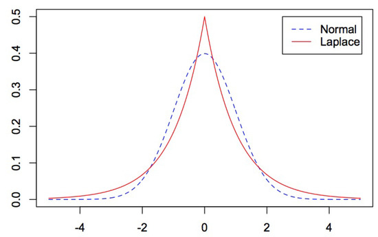
Figure 1.
The probability density funcitions of two distributions for mean=0, variance=1, .
We will introduce more detail about asymmetric Laplace distribution and the essential properties in Section 2. Next, in Section 3, VaR and CVaR of Asymmetric Laplace distribution are given. In Section 4, we apply the AL model to currency exchange rates data, showing the good fit of our model by comparing with normal and nonparametric models. We compute the Value-at-Risk (VaR) and Conditional Value-at-Risk (CVaR) from each model. Then, Section 5 includes conclusions and limitations as well as directions for future research.
2. Asymmetric Laplace Distribution
Because classical Gaussian distribution models are frequently not supported by real-life data due to fat tails and asymmetry prevalent in financial data, the Laplace and related distributions are natural candidates to replace Gaussian models and processes in modeling these data [20]. Since Laplace distributions can account for leptokurtic and skewed data [21], it is also used to fit the marginal distribution function, which will then be used in a copula function [22].
Definition 3.
A random variable Y is said to have an asymmetric Laplace (AL) distribution if there exist parameters and such that the characteristic function of Y has the form
We denote the distribution Y by and write .
Remark 1.
For some special cases:
- (1)
- If , then for every and the distribution is degenerate at 0.
- (2)
- For and , we have an exponential r.v. with mean μ (concentrated on ) for and on for .
- (3)
- For and , we have a symmetric Laplace distribution with mean θ and variance .
The characteristic function with can be expressed in the following manner:
where the additional parameter is related to and is as follows:
while
Therefore, we can give another definition of the Asymmetric Laplace distribution in the parametrization, using notation .
Definition 4.
Random variable Y is said to be distributed as Asymmetric Laplace distribution with location parameter θ, scale parameter , and skewness parameter , and denote the PDF and CDF of an distribution respectively. Then
and
Remark 2.
Note that since θ is simply a location parameter, we shall often assume , and for , we obtain the PDF and CDF of the symmetric Laplace distribution.
The following relations are often used:
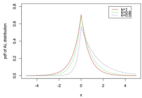
The definitions of Asymmetric Laplace distribution’s PDF with a different κ plot are shown in Figure 2.
Figure 2.
Different AL densities plot with .
A symmetric Laplace random variable can be regarded (informally) as a normal random variable with mean zero and variance that is an exponentially distributed random variable. AL r.v. values admit a similar interpretation, where the mean is a random variable as well.
Proposition 1
(Mixture of normal distributions). Conditionally on V, the distribution of the risk factor Y is normal with the mean and variance V, i.e.,
where Z is a standard normal variable independent of a positive random variable V having the mean . The parameter γ controls the correlation between the risk factor Y and the stochastic variance V.
Then, the distribution of the risk factor becomes Asymmetric Laplace distribution .
Proposition 2
(Moment-generating function). If , then the moment generating function of Y is
Proposition 3
(Cumulants). The cumulants of an can be stated as
The mean and variance of Y, which coincide with the first and second cumulants, respectively, are
Proposition 4
(Coefficients of kurtosis and skewness). The coefficient of skewness is a measure of symmetry defined by for a random variable Y with a finite third moment and a standard deviation greater than zero
The coefficient of skewness, defined by above, is a scale-independent measure of symmetry. Its value is zero for the symmetric Laplace distribution, as it is for any symmetric distribution with a finite third moment and greater than zero standard deviation.
For an distribution, the coefficient of skewness is nonzero, unless (). In terms of κ, its value is
The absolute value of is confined by two, and when the value of κ grows within the range of , the corresponding value of falls monotonically from 2 to −2, as seen in the graph.
For random variable Y with a finite fourth moment, the is defined as
This statistic measures the peaking and tailing of a normal distribution (correctly adjusted so that for a normal distribution), and it is completely independent of the scale. If , the distribution is considered to be Leptokurtic, which has heavy tails and a higher peakiness; otherwise, the distribution is said to be Platykurtic.
For an distribution, the kurtosis of AL distribution is
As a result, the distribution is leptokurtic with ranging from 3 (the smallest value for the Symmetric Laplace distribution with ) to 6 (the highest value for the limiting exponential distribution when ).
Proposition 5
(Quantiles). Let be the quantile of an distribution. Then we have
Again, the VaR can be explicitly computed as the quantiles of Asymmetric Laplace distribution.
3. VaR and CVaR for AL Distribution
Let , where are unknown parameters. Then, for upper quantile , VaR and CVaR can be obtained as
and
The explicit expressions of maximum likelihood estimations of the parameters and are given in Samuel Kotz et al. (2001) [19], provided the value of is known.
Consider a random sample form , the corresponding MLEs of the and can be written as follows:
where and .
Let and , the MLEs of and can be expressed equivalently as
4. Application
In this section, we present an application of the Asymmetric Laplace distribution presented in the previous section in modeling some financial data. Actually, numerous researchers have studied the Laplace and related probability distributions in the context of financial data modeling. Traditionally, this type of data was described using a Gaussian distribution, but because financial data are fat-tailed and sharp-peaked, this is no longer the case. It is required to search for a probability distribution that can account for the skewness and kurtosis that deviate from a Gaussian distribution in order to solve the problem. Since the Asymmetric Laplace can account for the leptokurtic behavior, it is a natural choice, which can be coincided as the first choice for skewed and kurtotic data [23].
Here, we will illustrate an application of the Asymmetric Laplace distribution on modeling financial data. The observations were the daily currency exchange rate covering the period from 1 January 2017 to 1 January 2021. In comparison to the United States dollar, four different currencies are available: the Australian dollar, the Canadian dollar, the European euro, and the United Kingdom pound. It is the natural logarithm of the price ratio for two consecutive days that is of importance, and the data were processed in this manner, yielding values for each currency.
We model the data with nonparametric estimation, normal distribution, and Asymmetric Laplace distribution by using the maximum likelihood estimations to obtain distributional fits. For nonparametric estimation, we used Kernel Density Estimation to fit the log-return data directly. Next, we have employed the well-known standard estimators for the mean and variance in the normal model (given in Table 1). Consequently, using the AL model, we have approximated the scale parameter as well as the skewness parameter , as shown in Table 2 below. Finally, we plot the results in Figure 3, Figure 4, Figure 5 and Figure 6.

Table 1.
Descriptive statistics for transformed daily currency exchange rate changes.
Table 2.
Descriptive statistics and estimated parameters and fitted distribution.
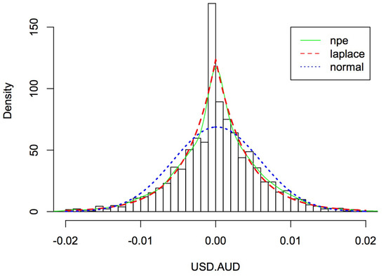
Figure 3.
The probability density functions of Australian dollar with different distributions.
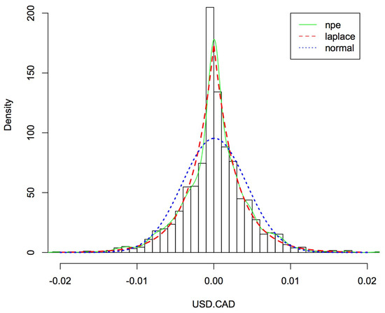
Figure 4.
The probability density functions of Canadian dollar with different distributions.
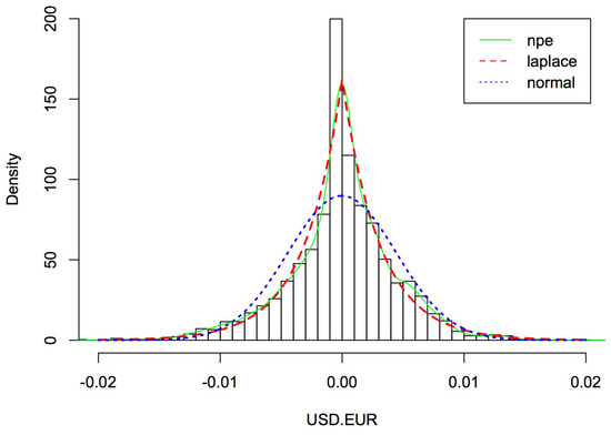
Figure 5.
The probability density functions of European euro with different distributions.
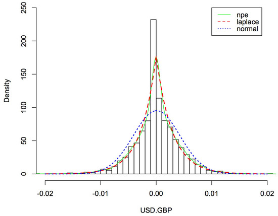
Figure 6.
The probability density functions of United Kingdom pound with different distributions.
The descriptive statistics for the transformed data fitted normal distribution appear in Table 1, including the mean, variance, and estimators of the coefficients of skewness and kurtosis introduced in Section 3; these parameters assess the distribution’s symmetry and peakness, respectively. Skewed (skewness larger than 0) and leptokurtic (adjusted kurtosis greater than 0) distributions of currency exchange rates appear to be present in the empirical distributions. Table 2 shows the estimated parameters and , and the above descriptive statistics fitted distribution with (assuming ) and .
Figure 3, Figure 4, Figure 5 and Figure 6 depict the histograms of the four currencies, the Australian dollar, the Canadian dollar, the European euro, and the United Kingdom pound, as well as the fitted nonparametric estimation, normal, and Asymmetric Laplace densities using the values in Table 1 and Table 2 (nonparametric estimation fitting data directly). Results in Figure 3, Figure 4, Figure 5 and Figure 6 show that the normal distribution does not appear to be a good fit for the data, as would be predicted. It appears that the empirical distributions have high peaks near zero and have tails that are thicker than those permitted by the normal distribution. As a result, we propose the Asymmetric Laplace model for the calculation of currency exchange rate. When it comes to computing, the AL model is straightforward, allows for asymmetry, and accurately depicts the leptocurticity of the empirical data [24].
Furthermore, in order to compare the fits of nonparametric estimation, the normal model, and the Asymmetric Laplace model, we compute the Kullback–Leibler Distance between the data and these three models, which is given in Table 3.
Table 3.
Kullback–Leibler distance between the data and nonparametric estimation, normal distribution, and AL distribution.
Table 4 shows the different results of Value-at-Risk (VaR) and Conditional Value-at- Risk (CVaR) with a given significant level , under nonparametric estimation, the normal model, and the Asymmetric Laplace model.
Table 4.
Kullback–Leibler distance between the data and nonparametric estimation, normal distribution, and AL distribution.
5. Conclusions
Our analysis shows that compared with the normal model, the VaR and CVaR under nonparametric estimation and the Asymmetric Laplace model performs better. In other words, the findings suggests that VaR and CVaR under the normal model could underestimate the true value of potential loss of the specific portfolio.
For the nonparametric estimation approach in computing VaR and CVaR, without a distribution to help determine future returns, we can assume that the past information will exactly replicate the future, simulation data for study. The strengths of the method are: (1) No forced assumption of a normal distribution has been made in the risk assessment; hence, all historical data have been completely integrated. (2) There was no need for a variance/covariance matrix to be used in order to compute the portfolio standard deviation. Consequently, the accuracy of this historical VaR estimate is only as good as the number of data points that are available to measure and the amount of time that has passed since the data were collected. It may turn out to be time-consuming or even impossible. However, in theory, if we had enough data to fully depict all of the crises events and changing business cycles that happened, this method would be preferable to the parametric method. The performance of the portfolio and the number of portfolios at risk would be known at any given time. However, even if we had historical data, there is no guarantee that it will ever completely duplicate itself historically if there is no known distribution.
For the parametric method in calculating VaR and CVaR, we used the AL model for currency exchange rates, because the AL model is simple to calculate, asymmetric, and captures the leptocurticity of the empirical data quite well. The disadvantage of parametric methods is that they are ineffective when the portfolio has discontinuous payoffs. Therefore, which methods we should choose, nonparametric estimation or parametric method with the Asymmetric Laplace model, to calculate VaR and CVaR still depends on different situations.
Finally, the methodology could also be generalized to incorporate and test some situations, especially stock price, interest rates, and commodity prices. The AL distribution is useful in capturing the peakedness, leptokurticity, and skewness inherent in such data. The result of this study suggests that AL could be an effective model to apply financial data to help firms perform better.
Author Contributions
Conceptualization, H.J., J.Z. and Y.L.; methodology, H.J. and J.Z.; software, H.J. and J.Z.; writing—original draft preparation, H.J.; writing—review and editing, Y.L. and J.Z. All authors have read and agreed to the published version of the manuscript.
Funding
This research was funded by the Ph.D Scientific Research Foundation of Liaocheng University (No. 321052022), and National Social Science Foundation of China (No. 20BJY074).
Institutional Review Board Statement
Not applicable.
Informed Consent Statement
Not applicable.
Data Availability Statement
Data are contained within the article.
Conflicts of Interest
The authors declare no conflict of interest.
References
- Bekiros, S.; Boubaker, S.; Nguyen, D.K.; Uddin, G.S. Black swan events and safe havens: The role of gold in globally integrated emerging markets. J. Int. Money Financ. 2017, 73, 317–334. [Google Scholar] [CrossRef] [Green Version]
- Shah, M.H.; Ullah, I.; Salem, S.; Ashfaq, S.; Rehman, A.; Zeeshan, M.; Fareed, Z. Exchange Rate Dynamics, Energy Consumption, and Sustainable Environment in Pakistan: New Evidence From Nonlinear ARDL Cointegration. Front. Environ. Sci. 2022, 9, 607. [Google Scholar] [CrossRef]
- Akram, R.; Majeed, M.T.; Fareed, Z.; Khalid, F.; Ye, C. Asymmetric effects of energy efficiency and renewable energy on carbon emissions of BRICS economies: Evidence from nonlinear panel autoregressive distributed lag model. Environ. Sci. Pollut. Res. Int. 2020, 27, 18254–18268. [Google Scholar] [CrossRef]
- Aracil, E.; Nájera-Sánchez, J.J.; Forcadell, F.J. Sustainable banking: A literature review and integrative framework. Financ. Res. Lett. 2021, 42, 101932. [Google Scholar] [CrossRef]
- Roy, A. Safety first and the holding of assets. Econometrica 1952, 20, 431–449. [Google Scholar] [CrossRef]
- Balbás, A.; Balbás, B.; Balbás, R. VaR as the CVaR sensitivity: Applications in risk optimization. J. Comput. Appl. Math. 2017, 309, 175–185. [Google Scholar] [CrossRef] [Green Version]
- Linsmeier, T.J.; Pearson, N.D. Risk Measurement: An Introduction to Value at Risk; Working paper; University of Illinois Urbana-Champaign: Champaign, IL, USA, 1996. [Google Scholar]
- Zhang, Q.; Gao, Y. Portfolio selection based on a benchmark process with dynamic value-at-risk constraints. J. Comput. Appl. Math. 2017, 313, 440–447. [Google Scholar] [CrossRef]
- Paramati, S.R.; Apergis, N.; Ummalla, M. Dynamics of renewable energy consumption and economic activities across the agriculture, industry, and service sectors: Evidence in the perspective of sustainable development. Environ. Sci. Pollut. Res. Int. 2018, 25, 1375–1387. [Google Scholar] [CrossRef]
- Acerbi, C.; Tasche, D. On the coherence of expected shortfall. J. Bank. Financ. 2002, 26, 1487–1503. [Google Scholar] [CrossRef] [Green Version]
- Rockafellar, R.T.; Uryasev, S. Conditional value-at-risk for general loss distributions. J. Bank. Financ. 2002, 26, 1443–1471. [Google Scholar] [CrossRef]
- Rockafellar, R.T.; Uryasev, S. Optimization of conditional value-at-risk. J. Risk 2000, 2, 21–42. [Google Scholar] [CrossRef] [Green Version]
- Artzner, P.; Delbaen, F.; Eber, J.M.; Heath, D. Coherent measures of risk. Math. Financ. 1999, 9, 203–228. [Google Scholar] [CrossRef]
- Szegö, G. Measures of risk. J. Bank. Financ. 2002, 26, 1253–1272. [Google Scholar] [CrossRef]
- Cvitanić, J.; Zapatero, F. Introduction to the Economics and Mathematics of Financial Markets; The MIT Press: London, UK, 2004. [Google Scholar]
- Zhou, J.; Aghili, N.; Ghaleini, E.N.; Bui, D.T.; Tahir, M.M.; Koopialipoor, M. A Monte Carlo simulation approach for effective assessment of flyrock based on intelligent system of neural network. Eng. Comput. 2019, 36, 713–723. [Google Scholar] [CrossRef]
- Chen, Q.; Gerlach, R.; Lu, Z. Bayesian Value-at-Risk and expected shortfall forecasting via the asymmetric Laplace distribution. Comput. Stat. Data Anal. 2012, 56, 3498–3516. [Google Scholar] [CrossRef]
- Bogdan, D.; Ştefana Maria, D.; Roxana, I. A Value-at-Risk forecastability indicator in the framework of a Generalized Autoregressive Score with “Asymmetric Laplace Distribution”. Financ. Res. Lett. 2022, 45, 102134. [Google Scholar] [CrossRef]
- Kotz, S.; Kozubowski, T.; Podgorski, K. The Laplace Distribution and Generalizations: A Revisit With Applications to Communications, Exonomics, Engineering, and Finance; Number 183; Springer: Berlin/Heidelberg, Germany, 2001. [Google Scholar]
- Yin, C.; Shen, Y.; Wen, Y. Exit problems for jump processes with applications to dividend problems. J. Comput. Appl. Math. 2013, 245, 30–52. [Google Scholar] [CrossRef]
- Franczak, B.C.; Browne, R.P.; McNicholas, P.D. Mixtures of Shifted AsymmetricLaplace Distributions. IEEE Trans. Pattern. Anal. Mach. Intell. 2014, 36, 1149–1157. [Google Scholar] [CrossRef] [PubMed] [Green Version]
- Nadaf, T.; Lotfi, T.; Shateyi, S. Revisiting the Copula-Based Trading Method Using the Laplace Marginal Distribution Function. Mathematics 2022, 10, 783. [Google Scholar] [CrossRef]
- Aryal, G.R. Study of Laplace and Related Probability Distributions and Their Applications. Ph.D. Thesis, University of South Florida, Tampa, FL, USA, 2006. [Google Scholar]
- Kozubowski, T.J.; Podgórski, K. Asymmetric Laplace laws and modeling financial data. Math. Comput. Model. 2001, 34, 1003–1021. [Google Scholar] [CrossRef]
Publisher’s Note: MDPI stays neutral with regard to jurisdictional claims in published maps and institutional affiliations. |
© 2022 by the authors. Licensee MDPI, Basel, Switzerland. This article is an open access article distributed under the terms and conditions of the Creative Commons Attribution (CC BY) license (https://creativecommons.org/licenses/by/4.0/).