Approximate Analytic–Numeric Fuzzy Solutions of Fuzzy Fractional Equations Using a Residual Power Series Approach

Abstract

In this article, we consider a reliable analytical and numerical approach to create fuzzy approximated solutions for differential equations of fractional order with appropriate uncertain initial data by the means of a residual error function. The concept of strongly generalized differentiability is utilized to introduce the fuzzy fractional derivatives. The proposed method provides a systematic scheme based on generalized Taylor expansion and minimization of the residual error function, so as to obtain the coefficients values of a fractional series based on the given initial data of triangular fuzzy numbers in the parametric form. The obtained approximated solutions are provided within an appropriate radius to the requisite domain in the form of rapidly convergent fractional series according to their parametric form. The method’s performance and applicability are verified by applying it on some numerical examples. The impact of $r$-levels and fractional order $\gamma$ is presented quantitatively and graphically, showing the coincidence between the exact and the fuzzy approximated solutions. Moreover, for reliability and accuracy, our obtained results are numerically compared with the exact solutions and with results obtained using other methods described in the literature. This indicates that the proposed approach overcomes the difficulties that appear in other approaches to create fractional series solutions for varied uncertain natural problems arising within the fields of applied physics and engineering.

1. Introduction

Uncertain models are one of the most significant parts of the fuzzy analysis theory and have rapidly developed in the last decades. With this, recent theoretical and applied aspects have been discussed by many mathematicians, including measure, symmetric and control theories, radiation transfer in a semi-infinite atmosphere, and so forth. They are considered influential tools for modeling several real-life situations and phenomena in which uncertainty results from several factors such as measurement errors, deficient data, and initial guesses. Recently, numerous publications have shown that fractional differential equations (FDEs) are a powerful and applicable instrument to describe the exact results of physical, applied mathematics, and engineering phenomena such as control systems, aerodynamics, signal processing, bio-mathematical problems, and others [1,2,3,4,5,6]. However, in some cases, the raw initial data are imprecise and could be replaced by uncertain initial data to obtain fuzzy FDEs. Therefore, fuzzy FDEs are crucial in fuzzy calculus and are a widespread model in various natural scientific areas, including population analysis, evaluation of weapon systems, civil engineering, and modeling in electro-hydraulics.

The concept of the fuzzy FDEs was first introduced by Agarwal et al. [7], who investigated fuzzy solutions for a certain class of fuzzy FDEs under the Hukuhara differentiability in the sense of Riemann–Liouville differentiability. Thereafter, many researchers have investigated solutions of ordinary fuzzy DEs and fuzzy FDEs (for more details, we refer to [8,9,10,11,12,13]). In addition, some mathematicians showed an interest in the existence and uniqueness of solutions for fuzzy FDEs. The authors of [14] proposed the existence and uniqueness of the solution to a fuzzy FDE under Hukuhara fractional Riemann–Liouville differentiability. Later, new and different techniques and methods were presented so that the existence and uniqueness of solutions for fuzzy FDEs were proved. Alikhani et al. [15] also confirmed the results of the existence and uniqueness of nonlinear fuzzy fractional integral and integro-differential equations by using the technique of upper and lower solutions. Additionally, these authors examined some related results about the existence and uniqueness of solutions to fuzzy FDEs under Caputo type-2 fuzzy fractional derivative and the definition of Laplace transform of type-2 fuzzy number-valued functions [16]. For instance, in [17], Salahshour et al. recommended some novel and different results for the existence and uniqueness of solutions of fuzzy FDEs.

Providing exact solutions to fuzzy FDEs is a difficult task. As a result, it is necessary to develop a robust numeric–analytic approach to deal with the complications of uncertain models and attain a precise mathematical framework for processing fuzzy initial value problems (IVPs) [18,19,20,21]. This analysis aimed to apply a recent treatment method, called the residual power series (RPS) method, to provide fuzzy approximated analytical solutions for a class of fuzzy FDEs under the concept of strongly generalized differentiability. This concept was introduced and discussed by Bede and Gal [22]. Later, it was developed and investigated (for more details see [23,24]). In fact, by utilizing strongly generalized differentiability, it is possible to find solutions for larger classes of fuzzy FDEs than by using other types of differentiability. More specifically, we here provide fuzzy approximated analytical solutions for the fuzzy fractional initial value problem (FFIVP) of the general form:

$$\{\begin{array}{cc}{D}_{a^{+}}^{\gamma }\phi \left(t\right)=F\left(t,\phi \left(t\right)\right),\hfill & a\le t\le b,\\ \phi \left(a\right)=\mu ,\hfill \end{array}$$

(1)

where $D_{a^{+}}^{\gamma }$ is the fuzzy Caputo fractional derivative of order $\gamma :0<\gamma \le 1$, $F:\left[a,b\right]\times {\mathbb{R}}_{\mathcal{F}}\to {\mathbb{R}}_{\mathcal{F}}$ is a continuous fuzzy-valued function, $\phi \left(t\right)$ is an unknown fuzzy analytical function to be determined, and $\mu \in {\mathbb{R}}_{\mathcal{F}}$, where ${\mathbb{R}}_{\mathcal{F}}$ stands for the set of fuzzy numbers on a real line.

In 2013, the scholar Abu Arqub [25] proposed the RPS as an effectively numeric–analytic approach and easily applied it to define the components of the suggested series solutions to a certain class of classical fuzzy DEs. Later, the RPS approach was developed for handling various kinds of FDEs [26,27,28,29]. This approach produces solutions to the given problem in the convergent generalized Taylor’s series formula without involving discretization, linearization, or perturbation [30,31,32]. It may be applied directly to given problems by selecting an appropriate value for the initial guess approximation. Recently, applications of the RPS approach for the simulation and creation of analytical solutions of FDEs, partial FDEs, and fuzzy FDEs have become popular and diverse, and numerous real-world problems have been studied and analyzed using the RPS approach, such as fractional stiff systems [33], time-fractional Fokker–Planck equations [34], time-fractional Whitham–Broer–Kaup equations [35], time-fractional Sharma–Tasso–Olever equation [34], fractional Newell–Whitehead–Segel equation [36], coupled fractional resonant Schrödinger equation [37], fractional foam drainage equation [38], and certain class of fractional systems of partial differential equations [39].

Approximate analytic–numeric techniques are considered to deal with fuzzy models of fractional PDEs, systems of fractional ODEs, and delay differential models. However, fuzzy fractional differential equations have not been investigated using the fractional power series method. Motivated by this, the primary objective of this work was to provide approximate analytic numerical solutions to fuzzy fractional initial value problems (IVPs) utilizing the RPS. The current article is organized as follows: Section 2 presents some of the well-known concepts and primary results of the fuzzy set theory and fuzzy fractional calculus theory. Section 3 discusses the formulation of the FFIVP (1) in the parametric form. Some FFIVPs are considered to demonstrate the efficiency and applicability of the RPS scheme presented in Section 4. Concluding remarks are outlined in Section 5.

2. Overview of the Fuzzy Fractional Calculus

In the subsequent section, we revise the most significant definitions and preliminary results related to the fuzzy fractional calculus. Assume that ${\mathbb{R}}_{\mathcal{F}}=\left\{\sigma :\mathbb{R}\to \left[0,1\right]\right\}$, where $\sigma$ is a fuzzy number satisfying the following conditions:

• $\sigma$ is normal; that is, there is an element $\zeta \in {\mathbb{R}}^m$ such that $\sigma \left(\zeta \right)=1$.
• $\sigma$ is convex; that is, for each ${\zeta }_1,{\zeta }_2\in {\mathbb{R}}^m$ and $0\le \theta \le 1$, we have $\sigma \left(\theta {\zeta }_1+\left(1-\theta \right){\zeta }_2\right)\ge \min \left(\sigma \left({\zeta }_1\right),\sigma \left({\zeta }_2\right)\right)$.
• $\sigma$ is upper semi-continuous.
• The closure of $\mathrm{supp}\left(\sigma \right)$ is a compact subset, where $\mathrm{supp}\left(\sigma \right)=\left\{\zeta \in {\mathbb{R}}^m:\sigma \left(\zeta \right)>0\right\}$.
• ${\mathbb{R}}_{\mathcal{F}}$ is the fuzzy numbers set.

For $r\in \left(0,1\right]$, the $r$-level representation of the fuzzy number $\sigma$ is defined by ${\left[\sigma \right]}^r=\left\{\zeta \in {\mathbb{R}}^m:\sigma \left(\zeta \right)>r\right\}.$ Then, $\sigma \in {\mathbb{R}}_{\mathcal{F}}$ if the $r$-level representation is a compact convex subset of $\mathbb{R}$. So, if $\sigma \in {\mathbb{R}}_{\mathcal{F}}$, then ${\left[\sigma \right]}^r=\left[{\sigma }_{1r},{\sigma }_{2r}\right]$, such that ${\sigma }_{1r}=\min \left\{\zeta :\zeta \in {\left[\sigma \right]}^r\right\}$, and ${\sigma }_{2r}=\max \left\{\zeta :\zeta \in {\left[\sigma \right]}^r\right\}$.

Definition 1.

Ref. [40] A triangular fuzzy number $\sigma$ is defined as a fuzzy set in ${\mathbb{R}}_{\mathcal{F}}$, which is given by $\sigma =\left(s,t,u\right)\in {\mathbb{R}}^3$, with $s\le t\le u,$ where the lower bound ${\sigma }_{1r}=s+\left(t-s\right)$, and the upper bound ${\sigma }_{2r}=u-\left(u-t\right)r$ are the endpoints of the $r$-level representation for each $r\in \left[0,1\right]$.

The Hausdorff distance between two arbitrary fuzzy numbers $\sigma$ and $\vartheta$ is defined as a mapping $d_H:{\mathbb{R}}_{\mathcal{F}}\times {\mathbb{R}}_{\mathcal{F}}\to {\mathbb{R}}^{+}{\displaystyle \cup }\left\{0\right\}$ and given by $d_h\left(\sigma ,\vartheta \right)={\sup }_{0\le r\le 1} \max \left\{{\sigma }_{1r}-{\vartheta }_{1r},{\sigma }_{2r}-{\vartheta }_{2r}\right\}$, where the $r$-level representations of $\sigma$ and $\vartheta$ are ${\left[\sigma \right]}^r=\left[{\sigma }_{1r},{\sigma }_{2r}\right]$ and ${\left[\vartheta \right]}^r=\left[{\vartheta }_{1r},{\vartheta }_{2r}\right]$, respectively.

Definition 2.

Ref. [22] Let $\phi :\left(a,b\right)\to {\mathbb{R}}_{\mathcal{F}}$ and fix $t_0\in \left[a,b\right].$ One can say $\phi$ is strongly generalized differentiable at $t_0$, if there is an element ${\phi }^{\prime }\left(t_0\right)\in {\mathbb{R}}_{\mathcal{F}}$ such that either:

• The $\mathscr{H}$-differences $\phi \left(t_0+\eta \right)\ominus \phi \left(t_0\right),\phi \left(t_0\right)\ominus \phi \left(t_0-\eta \right)$ exist, $\forall$ $\eta >0$, sufficiently approach to 0, and $\underset{\eta \to 0^{+}}{\lim }\frac{\phi \left(t_0+\eta \right)\ominus \phi \left(t_0\right)}{\eta }={\phi }^{\prime }\left(t_0\right)=\underset{\eta \to 0^{+}}{\lim }\frac{\phi \left(t_0\right)\ominus \phi \left(t_0-\eta \right)}{\eta },$
  or
• The $\mathscr{H}$-differences $\phi \left(t_0\right)\ominus \phi \left(t_0+\eta \right),\phi \left(t_0-\eta \right)\ominus \phi \left(t_0\right)$ exist $\forall$ $\eta >0$, sufficiently approach to 0, and $\underset{\eta \to 0^{+}}{\lim }\frac{\phi \left(t_0\right)\ominus \phi \left(t_0+\eta \right)}{-\eta }={\phi }^{\prime }\left(t_0\right)=\underset{\eta \to 0^{+}}{\lim }\frac{\phi \left(t_0-\eta \right)\ominus \phi \left(t_0\right)}{-\eta }$.
  where the limits here are taken in the complete metric space $\left({\mathbb{R}}_{\mathcal{F}},d_H\right)$.

Remark 1.

One can say $\phi$ is differentiable on $\left(a,b\right)$, when $\phi$ is differentiable for any point $t\in \left(a,b\right)$. Furthermore:

• $\phi$ is (1)-differentiable on $\left(a,b\right)$, and its derivative of $\phi$ at $t=t_0$ is given by ${\phi }^{\prime }\left(t_0\right)=D_1^1\phi \left(t_0\right)$, when $\phi$ is differentiable in terms of the first condition of Definition 2.
• $\phi$ is (2)-differentiable on $\left(a,b\right)$, and its derivative of $\phi$ at $t=t_0$ is given by ${\phi }^{\prime }\left(t_0\right)=D_2^1\phi \left(t_0\right)$, when $\phi$ is differentiable in terms of the second condition of Definition 2.

Definition 3.

Ref. [17] Let $\phi :\left[a,b\right]\to {\mathbb{R}}_{\mathcal{F}}$ and $\phi \in C^{\mathcal{F}}\left[a,b\right]{\displaystyle \cap }{L}^{\mathcal{F}}\left[a,b\right]$. One can say $\phi$ is Caputo fuzzy $H$-differentiable at $t$ when $D_{a^{+}}^{\gamma }\phi \left(t\right)=\frac{1}{\Gamma \left(1-\gamma \right)}{\int }_a^t\frac{{\phi }^{\prime }\left(\tau \right)}{{\left(t-\tau \right)}^{\gamma }}d\tau$ exists, where $0<\gamma \le 1$.

Remark 2.

We say that $\phi$ is Caputo $\left[\left(1\right)\text{-}\gamma \right]\text{-}$differentiable if $\phi$ is (1)-differentiable, and $\phi$ is Caputo $\left[\left(2\right)\text{-}\gamma \right]\text{-}$differentiable if $\phi$ is (2)-differentiable.

Theorem 1.

Ref. [17] Let $\phi :\left[a,b\right]\to {\mathbb{R}}_{\mathcal{F}}$ and $\phi \in C^{\mathcal{F}}\left[a,b\right]$, for $\gamma \in \left(0,1\right]$ $.$ Then, the fuzzy Caputo fractional derivative exists on $\left(a,b\right)$ for each $r\in \left[0,1\right]$, such that

• ${[D_{a^{+}}^{\gamma }\phi \left(t\right)]}^r=\left[D_{a^{+}}^{\gamma }{\phi }_{1r}\left(t\right),D_{a^{+}}^{\gamma }{\phi }_{2r}\left(t\right)\right]$, when $\phi$ is (1)-differentiable.
• ${[D_{a^{+}}^{\gamma }\phi \left(t\right)]}^r=\left[D_{a^{+}}^{\gamma }{\phi }_{2r}\left(t\right),D_{a^{+}}^{\gamma }{\phi }_{1r}\left(t\right)\right]$, when $\phi$ is (2)-differentiable.

Definition 4.

Ref. [29] A power series representation at $t=a$ has the following form

$${\displaystyle \sum }_{n=0}^{\infty }{c}_n\left(t-a\right){}^{n\gamma },0\le n-1<\gamma \le n,$$

It is called a fractional series (FS), where $t\ge a$ and $c_n$’s are called the coefficients of the series.

3. Fuzzy Fractional Initial Value Problems

In this section, we study a certain class of FFIVPs in the meaning of Caputo’s fuzzy H-differentiability throughout converting the main problem from the fuzzy environment into a crisp environment based on the differentiability type. Furthermore, we present an algorithm to solve the new system which consists of two fractional initial value problems (FIVPs).

The formulation of the target problem is the significant part of the procedure. Anyhow, to create the fuzzy solution of the FFIVPs, we reformulate (1) based on the type of differentiability in the $r$-level representation as follows:

$$\{\begin{array}{c}{\left[D_{a^{+}}^{\gamma }\phi (t)\right]}^r={\left[F\left(t,\phi \left(t\right)\right)\right]}^r,a\le t\le b,\hfill \\ {\left[\phi \left(a\right)\right]}^r={\left[\mu \right]}^r,\hfill \end{array}$$

(2)

where

${\left[D_{a^{+}}^{\gamma }\phi \left(t\right)\right]}^r=\left[D_{a^{+}}^{\gamma }{\phi }_{1r}\left(t\right),D_{a^{+}}^{\gamma }{\phi }_{2r}\left(t\right)\right]$, ${\left[\mu \right]}^r=\left[{\mu }_{1r},{\mu }_{2r}\right]$, and

${\left[F\left(t,\phi \left(t\right)\right)\right]}^r=[F_{1r}\left(t,{\phi }_{1r}\left(t\right),{\phi }_{2r}\left(t\right)\right),F_{2r}(t,{\phi }_{1r}\left(t\right),{\phi }_{2r}\left(t\right)]$, for $r\in \left[0,1\right]$, and $\gamma \in \left(0,1\right]$.

For $n\in \left\{1,2\right\}$, the $\left(n\right)$-solution of FFIVPs (1) is a fuzzy function $\phi :\left[a,b\right]\to {\mathbb{R}}_{\mathcal{F}}$ that has Caputo [$\left(n\right)\text{-}\gamma$]-differentiable and satisfies the fuzzy FIVPs (1). The next algorithm (Algorithm 1) along with Theorem 1 assisted us to find these solutions, ignoring the fuzzy settings approach:

$\mathrm{Algorithm}1:\mathrm{To}\mathrm{determine}\mathrm{the}\left(n\right)$-solutions of FFIVPs (1), we considered the following cases:

Case 1: Under Caputo [(1)-$\gamma$]-differentiable, the FFIVPs (1) converts to the following FIVPs system

$$\{\begin{array}{l}{D}_{a^{+}}^{\gamma }{\phi }_{1r}\left(t\right)=F_{1r}\left(t,{\phi }_{1r}\left(t\right),{\phi }_{2r}\left(t\right)\right),\\ D_{a^{+}}^{\gamma }{\phi }_{2r}\left(t\right)=F_{2r}\left(t,{\phi }_{1r}\left(t\right),{\phi }_{2r}\left(t\right)\right),\\ {\phi }_{1r}\left(a\right)={\mu }_{1r},\mathrm{and}{\phi }_{2r}\left(a\right)={\mu }_{2r}.\end{array}$$ (3)

Then, we used the following procedure:

First: Solve the system (3) for ${\phi }_{1r}\left(t\right)$ and ${\phi }_{2r}\left(t\right)$.

Second: Ensure that $\left[{\phi }_{1r}\left(t\right),{\phi }_{2r}\left(t\right)\right]$ and $\left[D_{a^{+}}^{\gamma }{\phi }_{1r}\left(t\right),D_{a^{+}}^{\gamma }{\phi }_{2r}\left(t\right)\right]$ are valid level sets for each $r\in \left[0,1\right]$.

Third: Construct the (1)-solution, $\phi \left(t\right),\mathrm{whose}r\text{-}\mathrm{level}\mathrm{representation}\mathrm{is}\left[{\phi }_{1r}\left(t\right),{\phi }_{2r}\left(t\right)\right]$.

Case 2: Under Caputo [(2)-$\gamma$]-differentiable, the FFIVPs (1) converts to the following FIVPs system:

$$\{\begin{array}{l}{D}_{a^{+}}^{\gamma }{\phi }_{1r}\left(t\right)=F_{2r}\left(t,{\phi }_{1r}\left(t\right),{\phi }_{2r}\left(t\right)\right),\\ D_{a^{+}}^{\gamma }{\phi }_{2r}\left(t\right)=F_{1r}\left(t,{\phi }_{1r}\left(t\right),{\phi }_{2r}\left(t\right)\right),\\ {\phi }_{1r}\left(a\right)={\mu }_{1r},\mathrm{and}{\phi }_{2r}\left(a\right)={\mu }_{2r}.\end{array}$$ (4)

Then, we performed the following procedure:

First: Solve the system (4) for ${\phi }_{1r}\left(t\right)$ and ${\phi }_{2r}\left(t\right)$.

Second: Ensure that $\left[{\phi }_{1r}\left(t\right),{\phi }_{2r}\left(t\right)\right]\mathrm{and}\left[D_{a^{+}}^{\gamma }{\phi }_{2r}\left(t\right),D_{a^{+}}^{\gamma }{\phi }_{1r}\left(t\right)\right]\mathrm{are}\mathrm{valid}\mathrm{level}\mathrm{sets}\mathrm{for}\mathrm{each}r\in \left[0,1\right]$.

Third: Construct the (2)-solution, $\phi \left(t\right),\mathrm{whose}r\text{-}\mathrm{level}\mathrm{representation}\mathrm{is}\left[{\phi }_{1r}\left(t\right),{\phi }_{2r}\left(t\right)\right]$.

Remark 3.

Let $n\in \left\{1,2\right\}$ and let ${[\phi \left(t\right)]}^r=\left[{\phi }_{1r}\left(t\right),{\phi }_{2r}\left(t\right)\right]$ be an $\left(n\right)$-solution of FFIVPs (1) on $\left[a,b\right]$. Then, ${\phi }_{1r}\left(t\right)$ and ${\phi }_{2r}\left(t\right)$ will be the solutions to the $\left(n\right)$-corresponding FIVPs systems.

Remark 4.

Let $n\in \left\{1,2\right\}$ and let ${\phi }_{1r}\left(t\right)$, ${\phi }_{2r}\left(t\right)$ represent the solutions of $\left(n\right)$-corresponding FIVPs systems for each $r\in \left[0,1\right]$. If ${[\phi \left(t\right)]}^r=\left[{\phi }_{1r}\left(t\right),{\phi }_{2r}\left(t\right)\right]$ has valid level sets and $\phi \left(t\right)$ is Caputo [$\left(n\right)\text{-}\gamma$]-differentiable, then $\phi \left(t\right)$ is an $\left(n\right)$-solution of FFIVPs (1) on $\left[a,b\right]$.

4. Application of the RPS Method to Solve FFIVPs

In this section, the fundamental principle of the proposed technique is introduced to predict and obtain analytical solutions for FFIVPs (1). The RPS approach provides an approximate solution by substituting the FPS expansion in its fractional truncated residual function.

Theorem 2.

Suppose that ${\phi }_{1r}\left(t\right)$ and ${\phi }_{2r}\left(t\right)$ have the following FS expansions about $t=a$:

$$\begin{gathered} {\phi }_{1r}\left(t\right)={\displaystyle \sum }_{n=0}^{\infty }{\omega }_n\frac{{\left(t-a\right)}^{n\gamma }}{\Gamma \left(n\gamma +1\right)}, \\ {\phi }_{2r}\left(t\right)={\displaystyle \sum }_{n=0}^{\infty }{\rho }_n\frac{{\left(t-a\right)}^{n\gamma }}{\Gamma \left(n\gamma +1\right)}. \end{gathered}$$

(5)

where $\gamma \in \left(0,1\right]$ and $t\in \left[a,a+R\right)$. If $D_{a^{+}}^{\gamma }{\phi }_{mr}\left(t\right)\in C\left[a,a+R\right)$, for $m\in \left\{1,2\right\}$, then the coefficients ${\omega }_n$ and ${\rho }_n$ will be written as ${\omega }_n=D_{a^{+}}^{n\gamma }{\phi }_{1r}\left(t\right)$, and ${\rho }_n=D_{a^{+}}^{n\gamma }{\phi }_{2r}\left(t\right)$, so that $D_{a^{+}}^{n\gamma }=D_{a^{+}}^{\gamma }·D_{a^{+}}^{\gamma }·\dots ·D_{a^{+}}^{\gamma }$ ($n$-times).

Proof: 

Let ${\phi }_{1r}\left(t\right)$ and ${\phi }_{2r}\left(t\right)$ be two arbitrary functions that could be expressed by an FS expansion (4). If we substitute $=$, into (5), one can notice that ${\omega }_0={\phi }_{1r}\left(a\right)$, ${\rho }_0={\phi }_{2r}\left(a\right)$, and ${\omega }_n={\rho }_n=0$, for $n=1,2,\dots$.

On other hand, operating $D_{a^{+}}^{\gamma }$ on both sides of (5) gives

$$\begin{gathered} D_{a^{+}}^{\gamma }{\phi }_{1r}\left(t\right)={\omega }_1+{\omega }_2\frac{{\left(t-a\right)}^{\gamma }}{\Gamma \left(\gamma +1\right)}+{\omega }_3\frac{{\left(t-a\right)}^{2\gamma }}{\Gamma \left(2\gamma +1\right)}+\dots , \\ {D}_{a^{+}}^{\gamma }{\phi }_{2r}\left(t\right)={\rho }_1+{\rho }_2\frac{{\left(t-a\right)}^{\gamma }}{\Gamma \left(\gamma +1\right)}+{\rho }_3\frac{{\left(t-a\right)}^{2\gamma }}{\Gamma \left(2\gamma +1\right)}+\dots . \end{gathered}$$

(6)

Then, by substituting $t=a$ into (6), we obtain ${\omega }_1=D_{a^{+}}^{\gamma }{\phi }_{1r}\left(a\right)$ and ${\rho }_1=D_{a^{+}}^{\gamma }{\phi }_{2r}\left(a\right)$.

Next, by applying $D_{a^{+}}^{\gamma }$ once on the resulting Equation (6):

$$\begin{gathered} D_{a^{+}}^{2\gamma }{\phi }_{1r}\left(t\right)=D_{a^{+}}^{\gamma }\left(D_{a^{+}}^{\gamma }{\phi }_{1r}\left(t\right)\right)={\omega }_2+{\omega }_3\frac{{\left(t-a\right)}^{\gamma }}{\Gamma \left(\gamma +1\right)}+{\omega }_4\frac{{\left(t-a\right)}^{3\gamma }}{\Gamma \left(3\gamma +1\right)}+\dots , \\ {D}_{a^{+}}^{2\gamma }{\phi }_{2r}\left(t\right)=D_{a^{+}}^{\gamma }\left(D_{a^{+}}^{\gamma }{\phi }_{2r}\left(t\right)\right)={\rho }_2+{\rho }_3\frac{{\left(t-a\right)}^{\gamma }}{\Gamma \left(\gamma +1\right)}+{\rho }_4\frac{{\left(t-a\right)}^{3\gamma }}{\Gamma \left(3\gamma +1\right)}+\dots . \end{gathered}$$

(7)

Here, if $t=a$ in (7), then the second coefficients of (5) will be ${\omega }_2=D_{a^{+}}^{2\gamma }{\phi }_{1r}\left(a\right)$ and ${\rho }_2=D_{a^{+}}^{2\gamma }{\phi }_{2r}\left(a\right)$. Likewise, by operating $D_{a^{+}}^{\gamma }$ on both sides of (6) and substituting $t=a$ into the resultant fractional equation the result is ${\omega }_3=D_{a^{+}}^{3\gamma }{\phi }_{1r}\left(a\right)$, and ${\rho }_3=D_{a^{+}}^{3\gamma }{\phi }_{2r}\left(a\right)$.

In the same way, we applied $D_{a^{+}}^{\gamma }$, $n$-times, and then considered $t=a$ in the resultant fractional equation, then the pattern of the unknown coefficients were obtained, and hence ${\omega }_n$ and ${\rho }_n$, in the FS expansions (5) had the general forms ${\omega }_n=D_{a^{+}}^{n\gamma }{\phi }_{1r}\left(t\right)$ and ${\rho }_n=D_{a^{+}}^{n\gamma }{\phi }_{2r}\left(t\right)$, for $n=0,1,2,3,\dots$. □

To reach our purpose, the following approach was used under Caputo [(1)-$\gamma$]-differentiable. Likewise, it can be applied to solve FFIVPs (1) under Caputo [(2)-$\gamma$]-differentiable.

Step A: According to Theorem 2, the RPS solutions of FIVPs system (3) at $a=0$ have the following FS forms:

$$\begin{gathered} {\phi }_{1r}\left(t\right)={\displaystyle \sum }_{n=0}^{\infty }{\omega }_n\frac{t^{n\gamma }}{\Gamma \left(n\gamma +1\right)}, \\ {\phi }_{2r}\left(t\right)={\displaystyle \sum }_{n=0}^{\infty }{\rho }_n\frac{t^{n\gamma }}{\Gamma \left(n\gamma +1\right)}. \end{gathered}$$

(8)

It is clear that ${\phi }_{1r}\left(t\right)$ and ${\phi }_{2r}\left(t\right)$ satisfy the initial condition of (3), then ${\phi }_{1r}\left(0\right)={\omega }_0={\mu }_{1r}$ and ${\phi }_{2r}\left(0\right)={\rho }_0={\mu }_{2r}$ will be the initial guess approximations for (3). So, the series solutions can be written as:

$$\begin{gathered} {\phi }_{1r}\left(t\right)={\mu }_{1r}+{\displaystyle \sum }_{n=1}^{\infty }{\omega }_n\frac{t^{n\gamma }}{\Gamma \left(n\gamma +1\right)}, \\ {\phi }_{2r}\left(t\right)={\mu }_{2r}+{\displaystyle \sum }_{n=1}^{\infty }{\rho }_n\frac{t^{n\gamma }}{\Gamma \left(n\gamma +1\right)}. \end{gathered}$$

(9)

Then, the $kth$-truncated series of the solutions ${\phi }_{1r}\left(t\right)$ and ${\phi }_{2r}\left(t\right)$ can be given as:

$$\begin{gathered} {\phi }_{k,1r}\left(t\right)={\mu }_{1r}+{\displaystyle \sum }_{n=1}^k{\omega }_n\frac{t^{n\gamma }}{\Gamma \left(n\gamma +1\right)}, \\ {\phi }_{k,2r}\left(t\right)={\mu }_{2r}+{\displaystyle \sum }_{n=1}^k{\rho }_n\frac{t^{n\gamma }}{\Gamma \left(n\gamma +1\right)}. \end{gathered}$$

(10)

Step B: Identify the so-called $k$-th residual functions of (3) as follows:

$$\begin{gathered} re{s}_{k,1r}\left(t\right)=D_{0^{+}}^{\gamma }{\phi }_{k,1r}\left(t\right)-F_{1r}\left(t,{\phi }_{k,1r}\left(t\right),{\phi }_{k,2r}\left(t\right)\right), \\ re{s}_{k,2r}\left(t\right)=D_{0^{+}}^{\gamma }{\phi }_{k,2r}\left(t\right)-F_{2r}\left(t,{\phi }_{k,1r}\left(t\right),{\phi }_{k,2r}\left(t\right)\right). \end{gathered}$$

(11)

As in [18], we note that $\underset{k\to \infty }{\lim }re{s}_{k,mr}\left(t\right)=re{s}_{mr}=0$, for $m=\left\{1,2\right\},$ and each $t\ge 0$. In fact, this leads to $D_{0^{+}}^{n\gamma }re{s}_{mr}\left(t\right)=0$, because of $D_{0^{+}}^{\gamma }C=0$, for any constant $C$. Further, $D_{0^{+}}^{n\gamma }re{s}_{mr}\left(t\right)$ and $D_{0^{+}}^{n\gamma }re{s}_{k,mr}\left(t\right)$ are equivalent at $t=0$, for each $n=0,1,2,\dots ,k$.

Step C: Substitute the $kth$-truncated series of the solutions ${\phi }_{1r}\left(t\right)$ and ${\phi }_{2r}\left(t\right)$ of (7) into the $k$-th residual functions $re{s}_{k,1r}$ and $re{s}_{k,2r}\left(t\right)$.

Step D: Apply the fractional operator $D_{0^{+}}^{\left(k-1\right)\gamma }$, for $k=1,2,\dots$ to both sides of the obtained fractional equations in Step C and then solve the following fractional systems for the target unknown coefficients:

$$\begin{gathered} D_{0^{+}}^{\left(k-1\right)\gamma }re{s}_{k,1r}\left(0\right)=0, \\ {D}_{0^{+}}^{\left(k-1\right)\gamma }re{s}_{k,2r}\left(0\right)=0. \end{gathered}$$

(12)

Step E: After solving (12), we obtained the forms of ${\omega }_n$ and ${\rho }_n$ in the expansions (10), and hence the $kth$-truncated series solutions were found.

Now, to find ${\omega }_1$ and ${\rho }_1$, we considered $k=1$, in (10), then substituted ${\phi }_{1,1r}\left(t\right)={\mu }_{1r}+{\omega }_1\frac{t^{\gamma }}{\Gamma \left(\gamma +1\right)}$ and ${\phi }_{1,2r}\left(t\right)={\mu }_{2r}+{\rho }_1\frac{t^{\gamma }}{\Gamma \left(\gamma +1\right)}$ into $re{s}_{1,1r}\left(t\right)$ and $re{s}_{1,2r}\left(t\right)$ of (11), that is,

$$\begin{gathered} re{s}_{1,1r}\left(t\right)=D_{0^{+}}^{\gamma }{\phi }_{1,1r}\left(t\right)-F_{1r}\left(t,{\phi }_{1,1r}\left(t\right),{\phi }_{1,2r}\left(t\right)\right) \\ ={\omega }_1-F_{1r}\left(t,{\mu }_{1r}+{\omega }_1\frac{t^{\gamma }}{\Gamma \left(\gamma +1\right)},{\mu }_{2r}+{\rho }_1\frac{t^{\gamma }}{\Gamma \left(\gamma +1\right)}\right), \\ re{s}_{1,2r}\left(t\right)=D_{0^{+}}^{\gamma }{\phi }_{1,2r}\left(t\right)-F_{2r}\left(t,{\phi }_{1,1r}\left(t\right),{\phi }_{1,2r}\left(t\right)\right) \\ ={\rho }_1-F_{2r}\left(t,{\mu }_{1r}+{\omega }_1\frac{t^{\gamma }}{\Gamma \left(\gamma +1\right)},{\mu }_{2r}+{\rho }_1\frac{t^{\gamma }}{\Gamma \left(\gamma +1\right)}\right). \end{gathered}$$

(13)

Then, by solving the system $re{s}_{1,1r}\left(0\right)=0$ and $re{s}_{1,2r}\left(0\right)=0$, we obtained ${\omega }_1=F_{1r}\left(0,{\mu }_{1r},{\mu }_{2r}\right)$ and ${\rho }_1=F_{2r}\left(0,{\mu }_{1r},{\mu }_{2r}\right)$. Thus, the 1st-FS approximated solutions for the system of FIVPs (3) can be written as:

$$\begin{gathered} {\phi }_{1,1r}\left(t\right)={\mu }_{1r}+F_{1r}\left(0,{\mu }_{1r},{\mu }_{2r}\right)\frac{t^{\gamma }}{\Gamma \left(\gamma +1\right)}, \\ {\phi }_{1,2r}\left(t\right)={\mu }_{2r}+F_{2r}\left(0,{\mu }_{1r},{\mu }_{2r}\right)\frac{t^{\gamma }}{\Gamma \left(\gamma +1\right)}. \end{gathered}$$

(14)

Similarly, to determine ${\omega }_2$ and ${\rho }_2$, we set $k=2$ in (10), then substituted ${\phi }_{2,1r}\left(t\right)={\mu }_{1r}+{\omega }_1\frac{t^{\gamma }}{\Gamma \left(\gamma +1\right)}+{\omega }_2\frac{t^{2\gamma }}{\Gamma \left(2\gamma +1\right)}$, and ${\phi }_{2,2r}\left(t\right)={\mu }_{2r}+{\rho }_1\frac{t^{\gamma }}{\Gamma \left(\gamma +1\right)}+{\rho }_2\frac{t^{2\gamma }}{\Gamma \left(2\gamma +1\right)}$ into $re{s}_{2,1r}\left(t\right)\mathrm{and}re{s}_{2,2r}\left(t\right)$ of Equation (11), as follows:

$$\begin{gathered} re{s}_{2,1r}\left(t\right)=D_{0^{+}}^{\gamma }\left({\mu }_{1r}+{\omega }_1\frac{t^{\gamma }}{\Gamma \left(\gamma +1\right)}+{\omega }_2\frac{t^{2\gamma }}{\Gamma \left(2\gamma +1\right)}\right)-F_{1r}\left(t,{\mu }_{1r}+{\omega }_1\frac{t^{\gamma }}{\Gamma \left(\gamma +1\right)}+{\omega }_2\frac{t^{2\gamma }}{\Gamma \left(2\gamma +1\right)},{\mu }_{2r}+{\rho }_1\frac{t^{\gamma }}{\Gamma \left(\gamma +1\right)}+{\rho }_2\frac{t^{2\gamma }}{\Gamma \left(2\gamma +1\right)}\right) \\ ={\omega }_1+{\omega }_2\frac{t^{\gamma }}{\Gamma \left(\gamma +1\right)}-F_{1r}\left(t,{\mu }_{1r}+{\omega }_1\frac{t^{\gamma }}{\Gamma \left(\gamma +1\right)}+{\omega }_2\frac{t^{2\gamma }}{\Gamma \left(2\gamma +1\right)},{\mu }_{2r}+{\rho }_1\frac{t^{\gamma }}{\Gamma \left(\gamma +1\right)}+{\rho }_2\frac{t^{2\gamma }}{\Gamma \left(2\gamma +1\right)}\right), \\ re{s}_{1,2r}\left(t\right)=D_{0^{+}}^{\gamma }\left({\mu }_{2r}+{\rho }_1\frac{t^{\gamma }}{\Gamma \left(\gamma +1\right)}+{\rho }_2\frac{t^{2\gamma }}{\Gamma \left(2\gamma +1\right)}\right)-F_{2r}\left(t,{\mu }_{1r}+{\omega }_1\frac{t^{\gamma }}{\Gamma \left(\gamma +1\right)}+{\omega }_2\frac{t^{2\gamma }}{\Gamma \left(2\gamma +1\right)},{\mu }_{2r}+{\rho }_1\frac{t^{\gamma }}{\Gamma \left(\gamma +1\right)}+{\rho }_2\frac{t^{2\gamma }}{\Gamma \left(2\gamma +1\right)}\right) \\ ={\rho }_1+{\rho }_2\frac{t^{\gamma }}{\Gamma \left(\gamma +1\right)}-F_{2r}\left(t,{\mu }_{1r}+{\omega }_1\frac{t^{\gamma }}{\Gamma \left(\gamma +1\right)}+{\omega }_2\frac{t^{2\gamma }}{\Gamma \left(2\gamma +1\right)},{\mu }_{2r}+{\rho }_1\frac{t^{\gamma }}{\Gamma \left(\gamma +1\right)}+{\rho }_2\frac{t^{2\gamma }}{\Gamma \left(2\gamma +1\right)}\right). \end{gathered}$$

(15)

By applying the operator $D_{0^{+}}^{\gamma }$ on both sides of (15), we obtained the $\gamma$-th Caputo fractional derivative of $re{s}_{2,1r}\left(t\right)$ and $re{s}_{2,2r}\left(t\right)$ and then we solved the obtained algebraic equations $D_{0^{+}}^{\gamma }re{s}_{2,1r}\left(0\right)=0$ and $D_{0^{+}}^{\gamma }re{s}_{2,2r}\left(0\right)=0$, obtaining ${\omega }_2=F_{1r}\left(0,{\omega }_1,{\rho }_1\right)$ and ${\rho }_2=F_{2r}\left(0,{\omega }_1,{\rho }_1\right)$. Therefore, the 2nd-FS approximated solutions for the system of FIVPs (3) can be written as:

$$\begin{gathered} {\phi }_{2,1r}\left(t\right)={\mu }_{1r}+F_{1r}\left(0,{\mu }_{1r},{\mu }_{2r}\right)\frac{t^{\gamma }}{\Gamma \left(\gamma +1\right)}+F_{1r}\left(0,{\omega }_1,{\rho }_1\right)\frac{t^{2\gamma }}{\Gamma \left(2\gamma +1\right)}, \\ {\phi }_{2,2r}\left(t\right)={\mu }_{2r}+F_{2r}\left(0,{\mu }_{1r},{\mu }_{2r}\right)\frac{t^{\gamma }}{\Gamma \left(\gamma +1\right)}+F_{2r}\left(0,{\omega }_1,{\rho }_1\right)\frac{t^{2\gamma }}{\Gamma \left(2\gamma +1\right)}. \end{gathered}$$

(16)

Thirdly, to obtain the coefficients $c_3$ and $d_3$, we considered $k=3$, in (10), then substituted ${\phi }_{3,1r}\left(t\right)={\mu }_{1r}+\sum _{n=1}^k{\omega }_n\frac{t^{n\gamma }}{\Gamma \left(n\gamma +1\right)}$, and ${\phi }_{3,2r}\left(t\right)={\mu }_{2r}+\sum _{n=1}^k{\rho }_n\frac{t^{n\gamma }}{\Gamma \left(n\gamma +1\right)}$ in $re{s}_{3,1r}\mathrm{and}re{s}_{3,2r}$ of (8); then, by computing $D_{0^{+}}^{2\gamma }re{s}_{3,1r}\left(t\right)$ and $D_{0^{+}}^{2\gamma }re{s}_{3,2r}\left(t\right)$ and using the facts $D_{0^{+}}^{2\gamma }re{s}_{3,1r}\left(0\right)=D_{0^{+}}^{2\gamma }re{s}_{3,2r}\left(0\right)=0,$ the coefficients ${\omega }_3$, and ${\rho }_3$ were obtained such that ${\omega }_3=F_{1r}\left(0,{\omega }_2,{\rho }_2\right)$ and ${\rho }_3=F_{2r}\left(0,{\omega }_2,{\rho }_2\right)$. Hence, the 3rd-FS approximated solutions for the system of FIVPs (3) can be summarized in the following expansions:

$${\phi }_{3,1r}\left(t\right)={\mu }_{1r}+F_{1r}\left(0,{\mu }_{1r},{\mu }_{2r}\right)\frac{t^{\gamma }}{\Gamma \left(\gamma +1\right)}+F_{1r}\left(0,{\omega }_1,{\rho }_1\right)\frac{t^{2\gamma }}{\Gamma \left(2\gamma +1\right)}+F_{1r}\left(0,{\omega }_2,{\rho }_2\right)\frac{t^{3\gamma }}{\Gamma \left(3\gamma +1\right)}$$

(17)

Using the same argument, the process can be repeated till the arbitrary order coefficients of the FS solutions for the system of FIVPs (3) are obtained. Hence, a higher degree of approximated solutions was achieved.

5. Numerical Experiments

In this section, we considered two FFIVPs of order $\gamma$ to demonstrate the efficiency and applicability of our algorithm. Here, all the symbolic and numerical computations were performed by using Mathematica 12.

Example 1.

Consider the following FFIVPs:

$$\{\begin{array}{ccc}{D}_{a^{+}}^{\gamma }\phi \left(t\right)=-\phi \left(t\right),\hfill & 0<\gamma \le 1,& t\in \left[0,1\right],\\ \phi \left(0\right)=\mu ,\hfill \end{array}$$

(18)

where $\mu =\left(2,3,4\right)$ is a fuzzy triangular number and has the$r$-level representations $\left[2+r,4-r\right]$ for $r\in \left[0,1\right]$. Based on Algorithm 1, the FFIVPs (18) will be transformed to one of the subsequent FIVPs systems:

Case 1:

The system of FIVPs corresponding to Caputo [(1)-$\gamma$]-differentiable is

$$\{\begin{array}{c}{D}_{0^{+}}^{\gamma }{\phi }_{1r}\left(t\right)=-{\phi }_{1r}\left(t\right),\\ D_{0^{+}}^{\gamma }{\phi }_{2r}\left(t\right)=-{\phi }_{2r}\left(t\right),\\ {\phi }_{1r}\left(0\right)=r+2,{\phi }_{2r}\left(0\right)=4-r.\end{array}$$

(19)

If $\gamma =1,$ then the $r$-level representations of the exact solutions for the FIVPs system (19) are given by:

$$\begin{gathered} {\phi }_{1r}\left(t\right)=\left(r+2\right)e^{-t}, \\ {\phi }_{2r}\left(t\right)=\left(4-r\right)e^{-t}. \end{gathered}$$

(20)

In light of the previous steps for the RPS algorithm, starting with ${\phi }_{0,1r}\left(0\right)=r+2$ and ${\phi }_{0,2r}\left(0\right)=4-r$, the $kth$-residual functions $re{s}_{k,1r}$ and $re{s}_{k,2r}$ for (19) will be defined as:

$$\begin{gathered} re{s}_{k,1r}\left(t\right)=D_{0^{+}}^{\gamma }{\phi }_{k,1r}\left(t\right)+{\phi }_{k,1r}\left(t\right), \\ re{s}_{k,2r}\left(t\right)=D_{0^{+}}^{\gamma }{\phi }_{k,2r}\left(t\right)+{\phi }_{k,2r}\left(t\right). \end{gathered}$$

(21)

where ${\phi }_{k,1r}$ and ${\phi }_{k,2r},$ indicating the $k$th-FS approximated solutions for (19), have the following forms:

$$\begin{gathered} {\phi }_{k,1r}\left(t\right)=\left(r+2\right)+{\displaystyle \sum }_{n=1}^k{\omega }_n\frac{t^{n\gamma }}{\Gamma \left(n\gamma +1\right)}, \\ {\phi }_{k,2r}\left(t\right)=\left(4-r\right)+{\displaystyle \sum }_{n=1}^k{\rho }_n\frac{t^{n\gamma }}{\Gamma \left(n\gamma +1\right)}. \end{gathered}$$

(22)

Now, to construct the 1st-FRPS-approximated solutions, consider $k=1$ in the residual Equation (21) to obtain $re{s}_{1,1r}\left(t\right)=D_{0^{+}}^{\gamma }\left(\left(r+2\right)+{\omega }_1\frac{t^{\gamma }}{\Gamma \left(\gamma +1\right)}\right)+\left(r+2\right)+{\omega }_1\frac{t^{\gamma }}{\Gamma \left(\gamma +1\right)}={\omega }_1+\left(r+2\right)+{\omega }_1\frac{t^{\gamma }}{\Gamma \left(\gamma +1\right)}$ and $Re{s}_{2,1r}\left(t\right)=D_{0^{+}}^{\gamma }\left(\left(4-r\right)+{\rho }_1\frac{t^{\gamma }}{\Gamma \left(\gamma +1\right)}\right)+\left(4-r\right)+{\rho }_1\frac{t^{\gamma }}{\Gamma \left(\gamma +1\right)}={\rho }_1+\left(4-r\right)+{\rho }_1\frac{t^{\gamma }}{\Gamma \left(\gamma +1\right)}$. Then, by using the fact $re{s}_{1,1r}\left(0\right)=re{s}_{1,2r}\left(0\right)=0$, we obtained ${\omega }_1=-\left(r+2\right), {\rho }_1=-\left(4-r\right)$. So, the 1st-FS approximated solutions for the FIVPs (19) can be expressed as ${\phi }_{1,1r}\left(t\right)=\left(r+2\right)-\left(r+2\right)\frac{t^{\gamma }}{\Gamma \left(\gamma +1\right)}$ and ${\phi }_{1,2r}\left(t\right)=\left(4-r\right)-\left(4-r\right)\frac{t^{\gamma }}{\Gamma \left(\gamma +1\right)}$.

Again, to find the 2nd-FS approximated solutions, put $k=2$, in (22), taking into account ${\omega }_1=-\left(r+2\right), {\rho }_1=-\left(4-r\right)$ and applying $D_{0^{+}}^{\gamma }$ in the resulting equations to obtain $D_{0^{+}}^{\gamma }re{s}_{2,1r}\left(t\right)={\omega }_2-\left(r+2\right)+{\omega }_2\frac{t^{\gamma }}{\Gamma \left(\gamma +1\right)}$ and $D_{0^{+}}^{\gamma }re{s}_{2,2r}\left(t\right)={\rho }_2-\left(4-r\right)+{\rho }_2\frac{t^{\gamma }}{\Gamma \left(\gamma +1\right)}$. Then, by considering that $D_{0^{+}}^{\gamma }re{s}_{2,1r}\left(0\right)=D_{0^{+}}^{\gamma }re{s}_{2,2r}\left(0\right)=0$, the coefficients ${\omega }_2$ and ${\rho }_2$ will be obtained, such that ${\omega }_2=r+2,{\rho }_2=4-r$. Hence, the 2nd-FS approximated solutions could be given as ${\phi }_{2,1r}\left(t\right)=\left(r+2\right)\left(1-\frac{t^{\gamma }}{\Gamma \left(\gamma +1\right)}+\frac{t^{2\gamma }}{\Gamma \left(2\gamma +1\right)}\right)$ and ${\phi }_{2,2r}\left(t\right)=\left(4-r\right)\left(1-\frac{t^{\gamma }}{\Gamma \left(\gamma +1\right)}+\frac{t^{2\gamma }}{\Gamma \left(2\gamma +1\right)}\right)$.

Similarly, by computing the operator $D_{0^{+}}^{2\gamma }$ of the 3rd-residual functions, one can get $D_{0^{+}}^{2\gamma }re{s}_{3,1r}\left(t\right)={\omega }_3+\left(r+2\right)+{\omega }_3\frac{t^{\gamma }}{\Gamma \left(\gamma +1\right)}$ and $D_{0^{+}}^{2\gamma }re{s}_{3,2r}\left(t\right)={\rho }_3+\left(4-r\right)+{\rho }_3\frac{t^{\gamma }}{\Gamma \left(\gamma +1\right)}$. Then, by solving the resultant fractional equations at $t=0$, we obtained ${\omega }_3=r+1, {\rho }_3=3-r$. Therefore, the 3rd-FS approximated solutions could be given as ${\phi }_{3,1r}\left(t\right)=\left(r+2\right)\left(1-\frac{t^{\gamma }}{\Gamma \left(\gamma +1\right)}+\frac{t^{2\gamma }}{\Gamma \left(2\gamma +1\right)}-\frac{t^{3\gamma }}{\Gamma \left(3\gamma +1\right)}\right)$ and ${\phi }_{3,2r}\left(t\right)=\left(4-r\right)\left(1-\frac{t^{\gamma }}{\Gamma \left(\gamma +1\right)}+\frac{t^{2\gamma }}{\Gamma \left(2\gamma +1\right)}-\frac{t^{3\gamma }}{\Gamma \left(3\gamma +1\right)}\right)$.

Using the same approach for $k=4$ and based on the fact that $D_{0^{+}}^{3\gamma }re{s}_{4,1r}\left(0\right)=D_{0^{+}}^{3\gamma }re{s}_{4,2r}\left(0\right)=0$, we obtained ${\omega }_4=r+1, {\rho }_4=4-r$. Depending on this, the 4th-FS approximated solutions can be written as ${\phi }_{4,1r}\left(t\right)=\left(r+2\right)\left(1-\frac{t^{\gamma }}{\Gamma \left(\gamma +1\right)}+\frac{t^{2\gamma }}{\Gamma \left(2\gamma +1\right)}-\frac{t^{3\gamma }}{\Gamma \left(3\gamma +1\right)}+\frac{t^{4\gamma }}{\Gamma \left(4\gamma +1\right)}\right)$ and ${\phi }_{4,2r}\left(t\right)=\left(4-r\right)\left(1-\frac{t^{\gamma }}{\Gamma \left(\gamma +1\right)}+\frac{t^{2\gamma }}{\Gamma \left(2\gamma +1\right)}-\frac{t^{3\gamma }}{\Gamma \left(3\gamma +1\right)}+\frac{t^{4\gamma }}{\Gamma \left(4\gamma +1\right)}\right)$. Moreover, depending on the fact that $D_{0^{+}}^{\left(k-1\right)\gamma }re{s}_{k,1r}\left(0\right)=D_{0^{+}}^{\left(k-1\right)\gamma }re{s}_{k,2r}\left(0\right)=0$ for $k=5,6,7,\dots$, the FS approximated solutions for (19) could be reformulated as:

$$\begin{gathered} {\phi }_{1r}\left(t\right)=\left(r+2\right)\left(1-\frac{t^{\gamma }}{\Gamma \left(\gamma +1\right)}+\frac{t^{2\gamma }}{\Gamma \left(2\gamma +1\right)}-\frac{t^{3\gamma }}{\Gamma \left(3\gamma +1\right)}+\frac{t^{4\gamma }}{\Gamma \left(4\gamma +1\right)}-\cdots \right) \\ =\left(\left(r+2\right){\displaystyle \sum }_{n=0}^{\infty }\frac{t^{n\beta }}{\Gamma \left(n\beta +1\right)}\right)=\left(r+2\right)E_{\gamma }\left(-t\right), \\ {\phi }_{2r}\left(t\right)=\left(4-r\right)\left(1-\frac{t^{\gamma }}{\Gamma \left(\gamma +1\right)}+\frac{t^{2\gamma }}{\Gamma \left(2\gamma +1\right)}-\frac{t^{3\gamma }}{\Gamma \left(3\gamma +1\right)}+\frac{t^{4\gamma }}{\Gamma \left(4\gamma +1\right)}-\cdots \right) \\ =\left(\left(r+2\right){\displaystyle \sum }_{n=0}^{\infty }\frac{t^{n\beta }}{\Gamma \left(n\beta +1\right)}\right)=\left(4-r\right)E_{\gamma }\left(-t\right). \end{gathered}$$

(23)

where $E_{\gamma }\left(t\right)$ is the Mittag–Leffler function.

In the case of $\gamma =1$, the FS expansions (23) could be reduced to the following forms:

$$\begin{gathered} {\phi }_{1r}\left(t\right)=\left(r+2\right)\left(1-t+\frac{t^2}{2}-\frac{t^3}{3!}+\frac{t^4}{4!}-\frac{t^5}{5!}+\frac{t^6}{6!}-\cdots \right)=\left(r+2\right)e^{-t}, \\ {\phi }_{2r}\left(t\right)=\left(4-r\right)\left(1-t+\frac{t^2}{2}-\frac{t^3}{3!}+\frac{t^4}{4!}-\frac{t^5}{5!}+\frac{t^6}{6!}-\cdots \right)=\left(4-r\right)e^{-t}. \end{gathered}$$

(24)

which coincide with the Taylor series expansions of the exact solutions ${\phi }_{1r}\left(t\right)=\left(r+2\right)e^{-t}$ and ${\phi }_{2r}\left(t\right)=\left(4-r\right)e^{-t}$.

Table 1 shows the lower and the upper bound solutions,${\phi }_{1r}\left(t\right)$ and ${\phi }_{2r}\left(t\right),$ of the 7th-FS approximated solutions for FIVPs (19) for different values of $\gamma$, when $r=1$.

Table 1. The (1)-approximated solutions of Example 1, case 1, for different values of $\gamma ,$ with $r=1$.

${\mathit{\gamma }}_{\mathit{i}}$	7th-FS Approximated Solutions, Case 1
$\frac{1}{4}$	${\phi }_{7,1r}\left(t\right)={\phi }_{7,2r}\left(t\right)=3+3t+\frac{2\sqrt{t}\left(3+2t\right)}{\sqrt{\pi }}-\frac{3t^{1/4}\left(5+4t\right)}{5\Gamma \left(\frac{5}{4}\right)}-\frac{3t^{3/4}\left(7+4t\right)}{7\Gamma \left(\frac{7}{4}\right)}.$
$\frac{1}{2}$	${\phi }_{7,1r}\left(t\right)={\phi }_{7,2r}\left(t\right)=3+\frac{1}{2}t\left(6+t\left(3+t\right)\right)-\frac{2\sqrt{t}\left(105+2t\left(35+2t\left(7+2t\right)\right)\right)}{35\sqrt{\pi }}.$
$\frac{3}{4}$	${\phi }_{7,1r}\left(t\right)={\phi }_{7,2r}\left(t\right)=3+\frac{t^3}{2}+\frac{4t^{3/2}\left(315+8t^3\right)}{315\sqrt{\pi }}-\frac{t^{3/4}\left(1155+64t^3\right)}{385\Gamma \left(\frac{7}{4}\right)}-\frac{t^{9/4}\left(4641+64t^3\right)}{1547\Gamma \left(\frac{13}{4}\right)}.$
$1$	${\phi }_{7,1r}\left(t\right)={\phi }_{7,2r}\left(t\right)=3-3t+\frac{3t^2}{2}-\frac{t^3}{2}+\frac{t^4}{4}-\frac{t^5}{20}+\frac{t^6}{120}-\frac{t^7}{840}.$

Case 2:

The system of FIVPs corresponding to Caputo [(2)-$\gamma$]-differentiable is

$$\{\begin{array}{c}{D}_{0^{+}}^{\gamma }{\phi }_{1r}\left(t\right)=-{\phi }_{2r}\left(t\right),\\ D_{0^{+}}^{\gamma }{\phi }_{2r}\left(t\right)=-{\phi }_{1r}\left(t\right),\\ {\phi }_{1r}\left(0\right)=r+2,{\phi }_{2r}\left(0\right)=4-r.\end{array}$$

(25)

If $\gamma =1,$ then the $r$-level representations of the exact solution for the FIVPs system (25) are given by:

$$\begin{gathered} {\phi }_{1r}\left(t\right)=3e^{-t}+\left(r-1\right)e^t, \\ {\phi }_{2r}\left(t\right)=3e^{-t}+\left(1-r\right)e^t. \end{gathered}$$

(26)

According to the RPS approach, starting with the 0th-FS approximated solutions ${\phi }_{0,1r}\left(0\right)=r+2,{\phi }_{0,2r}\left(0\right)=4-r$, the $k$th-FS approximated solutions of (25) take the forms:

$$\begin{gathered} {\phi }_{k,1r}\left(t\right)=\left(r+2\right)+{\displaystyle \sum }_{n=1}^k{\omega }_n\frac{t^{n\gamma }}{\Gamma \left(n\gamma +1\right)}, \\ {\phi }_{k,2r}\left(t\right)=\left(4-r\right)+{\displaystyle \sum }_{n=1}^k{\rho }_n\frac{t^{n\gamma }}{\Gamma \left(n\gamma +1\right)}. \end{gathered}$$

(27)

Thus, the $k$th-residual functions of (25) will be

$$\begin{gathered} re{s}_{k,1r}\left(t\right)=D_{0^{+}}^{\gamma }\left(\left(r+2\right)+{\displaystyle \sum }_{n=1}^k{\omega }_n\frac{t^{n\gamma }}{\Gamma \left(n\gamma +1\right)}\right)+\left(\left(4-r\right)+{\displaystyle \sum }_{n=1}^k{\rho }_n\frac{t^{n\gamma }}{\Gamma \left(n\gamma +1\right)}\right), \\ re{s}_{k,2r}\left(t\right)=D_{0^{+}}^{\gamma }\left(\left(4-r\right)+{\displaystyle \sum }_{n=1}^k{\rho }_n\frac{t^{n\gamma }}{\Gamma \left(n\gamma +1\right)}\right)+\left(\left(r+2\right)+{\displaystyle \sum }_{n=1}^k{\omega }_n\frac{t^{n\gamma }}{\Gamma \left(n\gamma +1\right)}\right) \end{gathered}$$

(28)

To obtain the values of the coefficients ${\omega }_n$ and ${\rho }_n$, $n=1,2,3,\dots ,k$, in FS expansions (27), solve the algebraic fractional system in ${\omega }_n$ and ${\rho }_n$ that was obtained considering $D_{0^{+}}^{\left(k-1\right)\gamma }re{s}_{k,1r}\left(0\right)=D_{0^{+}}^{\left(k-1\right)\gamma }re{s}_{k,2r}\left(0\right)=0,0<\gamma \le 1,k=1,2,3,\dots$.

Following the procedure of the RPS algorithm, the values of ${\omega }_n$, and ${\rho }_n$, $n=1,2,3,\dots ,k$ in (27) can be obtained as follows:

• For $k=1$, we had $re{s}_{1,1r}\left(t\right)=D_{0^{+}}^{\gamma }\left(\left(r+2\right)+{\omega }_1\frac{t^{\gamma }}{\Gamma \left(\gamma +1\right)}\right)+\left(4-r\right)+{\rho }_1\frac{t^{\gamma }}{\Gamma \left(\gamma +1\right)}={\omega }_1+\left(4-r\right)+{\rho }_1\frac{t^{\gamma }}{\Gamma \left(\gamma +1\right)}$, and $re{s}_{1,2r}\left(t\right)=D_{0^{+}}^{\gamma }\left(\left(4-r\right)+{\rho }_1\frac{t^{\gamma }}{\Gamma \left(\gamma +1\right)}\right)+\left(r+2\right)+{\omega }_1\frac{t^{\gamma }}{\Gamma \left(\gamma +1\right)}={\rho }_1+\left(r+2\right)+{\omega }_1\frac{t^{\gamma }}{\Gamma \left(\gamma +1\right)}$. Then, considering $re{s}_{1,1r}\left(0\right)=re{s}_{1,2r}\left(0\right)=0$, we obtained ${\omega }_1=-\left(4-r\right)$, ${\rho }_1=-\left(r+2\right)$.
• For $k=2$, we had $D_{0^{+}}^{\gamma }re{s}_{2,1r}\left(t\right)=D_{0^{+}}^{\gamma }\left(D_{0^{+}}^{\gamma }\left(\left(r+2\right)-\left(4-r\right)\frac{t^{\gamma }}{\Gamma \left(\gamma +1\right)}+{\omega }_2\frac{t^{2\gamma }}{\Gamma \left(2\gamma +1\right)}\right)+\left(4-r\right)-\left(r+2\right)\frac{t^{\gamma }}{\Gamma \left(\gamma +1\right)}+{\rho }_2\frac{t^{2\gamma }}{\Gamma \left(2\gamma +1\right)}\right)={\omega }_2-\left(r+2\right)+{\rho }_2\frac{t^{\gamma }}{\Gamma \left(\gamma +1\right)}$, and $D_{0^{+}}^{\gamma }re{s}_{2,2r}\left(t\right)=D_{0^{+}}^{\gamma }\left(D_{0^{+}}^{\gamma }\left(\left(4-r\right)-\left(r+2\right)\frac{t^{\gamma }}{\Gamma \left(\gamma +1\right)}+{\rho }_2\frac{t^{2\gamma }}{\Gamma \left(2\gamma +1\right)}\right)+\left(r+2\right)-\left(4-r\right)\frac{t^{\gamma }}{\Gamma \left(\gamma +1\right)}+{\omega }_2\frac{t^{2\gamma }}{\Gamma \left(2\gamma +1\right)}\right)={\rho }_2-\left(4-r\right)+{\omega }_2\frac{t^{\gamma }}{\Gamma \left(\gamma +1\right)}$. Lastly, by considering $D_{0^{+}}^{\gamma }re{s}_{2,1r}\left(0\right)=D_{0^{+}}^{\gamma }re{s}_{2,2r}\left(0\right)=0$, we obtained ${\omega }_2=\left(r+2\right)$, ${\rho }_2=\left(4-r\right)$.
• For $k=3$, we had $D_{0^{+}}^{2\gamma }re{s}_{3,1r}\left(t\right)=D_{0^{+}}^{2\gamma }\left(D_{0^{+}}^{\gamma }\left(\left(r+2\right)-\left(4-r\right)\frac{t^{\gamma }}{\Gamma \left(\gamma +1\right)}+\left(r+2\right)\frac{t^{2\gamma }}{\Gamma \left(2\gamma +1\right)}+{\omega }_3\frac{t^{3\gamma }}{\Gamma \left(3\gamma +1\right)}\right)+\left(4-r\right)-\left(r+2\right)\frac{t^{\gamma }}{\Gamma \left(\gamma +1\right)}+\left(4-r\right)\frac{t^{2\gamma }}{\Gamma \left(2\gamma +1\right)}+{\rho }_3\frac{t^{3\gamma }}{\Gamma \left(3\gamma +1\right)}\right)={\omega }_3+\left(4-r\right)+{\rho }_3\frac{t^{\gamma }}{\Gamma \left(\gamma +1\right)}$, and $D_{0^{+}}^{2\gamma }Re{s}_{3,2r}\left(t\right)=D_{0^{+}}^{2\gamma }\left(D_{0^{+}}^{\gamma }\left(\left(4-r\right)-\left(r+2\right)\frac{t^{\gamma }}{\Gamma \left(\gamma +1\right)}+\left(4-r\right)\frac{t^{2\gamma }}{\Gamma \left(2\gamma +1\right)}+{\rho }_3\frac{t^{3\gamma }}{\Gamma \left(3\gamma +1\right)}\right)+\left(r+2\right)-\left(4-r\right)\frac{t^{\gamma }}{\Gamma \left(\gamma +1\right)}+\left(r+2\right)\frac{t^{2\gamma }}{\Gamma \left(2\gamma +1\right)}+{\omega }_3\frac{t^{3\gamma }}{\Gamma \left(3\gamma +1\right)}\right)={\rho }_3+\left(r+2\right)+{\omega }_3\frac{t^{\gamma }}{\Gamma \left(\gamma +1\right)}$. Thus, by considering $D_{0^{+}}^{2\gamma }re{s}_{2,1r}\left(0\right)=D_{0^{+}}^{2\gamma }re{s}_{2,2r}\left(0\right)=0$, we obtained ${\omega }_3=-\left(4-r\right)$, ${\rho }_3=-\left(r+2\right)$.
• For $k=4$, we had $D_{0^{+}}^{3\gamma }re{s}_{4,1r}\left(t\right)=D_{0^{+}}^{3\gamma }\left(D_{0^{+}}^{\gamma }\left(\left(r+2\right)-\left(4-r\right)\frac{t^{\gamma }}{\Gamma \left(\gamma +1\right)}+\left(r+2\right)\frac{t^{2\gamma }}{\Gamma \left(2\gamma +1\right)}-\left(4-r\right)\frac{t^{\gamma }}{\Gamma \left(\gamma +1\right)}+{\omega }_4\frac{t^{4\gamma }}{\Gamma \left(4\gamma +1\right)}\right)+\left(4-r\right)-\left(r+2\right)\frac{t^{\gamma }}{\Gamma \left(\gamma +1\right)}+\left(4-r\right)\frac{t^{2\gamma }}{\Gamma \left(2\gamma +1\right)}-\left(r+2\right)\frac{t^{3\gamma }}{\Gamma \left(3\gamma +1\right)}+{\rho }_4\frac{t^{4\gamma }}{\Gamma \left(4\gamma +1\right)}\right)={\omega }_4-\left(r+2\right)+{\rho }_4\frac{t^{\gamma }}{\Gamma \left(\gamma +1\right)}$, and $D_{0^{+}}^{3\gamma }re{s}_{4,2r}\left(t\right)=D_{0^{+}}^{3\gamma }\left(D_{0^{+}}^{\gamma }\left(\left(4-r\right)-\left(r+2\right)\frac{t^{\gamma }}{\Gamma \left(\gamma +1\right)}+\left(4-r\right)\frac{t^{2\gamma }}{\Gamma \left(2\gamma +1\right)}-\left(r+2\right)\frac{t^{3\gamma }}{\Gamma \left(3\gamma +1\right)}+{\rho }_4\frac{t^{4\gamma }}{\Gamma \left(4\gamma +1\right)}\right)+\left(r+2\right)-\left(4-r\right)\frac{t^{\gamma }}{\Gamma \left(\gamma +1\right)}+\left(r+2\right)\frac{t^{2\gamma }}{\Gamma \left(2\gamma +1\right)}+\left(4-r\right)\frac{t^{\gamma }}{\Gamma \left(\gamma +1\right)}+{\omega }_4\frac{t^{4\gamma }}{\Gamma \left(4\gamma +1\right)}\right)={\rho }_4-\left(4-r\right)+{\omega }_4\frac{t^{\gamma }}{\Gamma \left(\gamma +1\right)}$. Thus, by considering $D_{0^{+}}^{3\gamma }re{s}_{4,2r}\left(0\right)=D_{0^{+}}^{3\gamma }re{s}_{4,2r}\left(0\right)=0$, we obtained ${\omega }_4=\left(r+2\right)$, ${\rho }_4=\left(4-r\right)$.
• Likewise, for $k=5$ and considering $D_{0^{+}}^{4\gamma }re{s}_{5,1r}\left(0\right)=D_{0^{+}}^{4\gamma }re{s}_{5,2r}\left(0\right)=0$, the coefficients ${\omega }_5$ and ${\rho }_5$ will be obtained such that ${\omega }_5=-\left(4-r\right)$, ${\rho }_5=-\left(r+2\right)$.
• Continuing with this procedure and based upon $D_{0^{+}}^{\left(k-1\right)\gamma }re{s}_{k,1r}\left(0\right)=D_{0^{+}}^{\left(k-1\right)\gamma }re{s}_{k,2r}\left(0\right)=0$, $k=6,7,8$, the 8th-FS approximated solutions for IVPs (25) were obtained:

  $$\begin{gathered} {\phi }_{8,1r}\left(t\right)=\left(\left(r+2\right)-\left(4-r\right)\frac{t^{\gamma }}{\Gamma \left(\gamma +1\right)}+\left(r+2\right)\frac{t^{2\gamma }}{\Gamma \left(2\gamma +1\right)}-\left(4-r\right)\frac{t^{3\gamma }}{\Gamma \left(3\gamma +1\right)}+\left(r+2\right)\frac{t^{4\gamma }}{\Gamma \left(4\gamma +1\right)}-\left(4-r\right)\frac{t^{5\gamma }}{\Gamma \left(5\gamma +1\right)}+\left(r+2\right)\frac{t^{6\gamma }}{\Gamma \left(6\gamma +1\right)}-\left(4-r\right)\frac{t^{7\gamma }}{\Gamma \left(7\gamma +1\right)}+\left(r+2\right)\frac{t^{8\gamma }}{\Gamma \left(8\gamma +1\right)}\right), \\ {\phi }_{8,2r}\left(t\right)=\left(\left(4-r\right)-\left(r+2\right)\frac{t^{\gamma }}{\Gamma \left(\gamma +1\right)}+\left(4-r\right)\frac{t^{2\gamma }}{\Gamma \left(2\gamma +1\right)}-\left(r+2\right)\frac{t^{3\gamma }}{\Gamma \left(3\gamma +1\right)}+\left(4-r\right)\frac{t^{4\gamma }}{\Gamma \left(4\gamma +1\right)}-\left(r+2\right)\frac{t^{5\gamma }}{\Gamma \left(5\gamma +1\right)}+\left(4-r\right)\frac{t^{6\gamma }}{\Gamma \left(6\gamma +1\right)}-\left(r+2\right)\frac{t^{7\gamma }}{\Gamma \left(7\gamma +1\right)}+\left(4-r\right)\frac{t^{8\gamma }}{\Gamma \left(8\gamma +1\right)}\right). \end{gathered}$$

In particular, when $\gamma =1$, the FS approximated solutions for (25) could be expressed as

$$\begin{gathered} {\phi }_{1r}\left(t\right)=\underset{k\to \infty }{\lim }{\phi }_{k,1r}\left(t\right)=\left(\left(r+2\right)-\left(4-r\right)t+\left(r+2\right)\frac{t^2}{2!}-\left(4-r\right)\frac{t^3}{3!}+\left(r+2\right)\frac{t^4}{4!}+\dots \right), \\ {\phi }_{2r}\left(t\right)=\underset{k\to \infty }{\lim }{\phi }_{k,2r}\left(t\right)=\left(\left(4-r\right)-\left(r+2\right)t+\left(4-r\right)\frac{t^2}{2!}-\left(r+2\right)\frac{t^3}{3!}+\left(4-r\right)\frac{t^4}{4!}+\dots \right). \end{gathered}$$

which agrees with the Maclurain series expansions of the exact solutions ${\phi }_{1r}\left(t\right)=3e^{-t}+\left(r-1\right)e^t$ and ${\phi }_{2r}\left(t\right)=3e^{-t}+\left(1-r\right)e^t$.

Utilizing the RPS method, the numerical results of the fuzzy 8th-FS approximated solutions $\left[{\phi }_{8,1r}\left(t\right),{\phi }_{8,2r}\left(t\right)\right]$ are shown in Table 2 of Example 1, case 1, for different values of $\gamma$ and a fixed value of the $r$-level. The effectiveness and reliability of the present method were also demonstrated via computing the absolute errors of the lower and upper approximated solutions and are presented in Table 3 of Example 1, case 2. From the table, we note the agreement between the obtained and the exact solutions at standard order $\gamma =1$.

Table 2. Numerical results of the 8th-FS approximated solutions $\left[{\phi }_{8,1r}\left(t\right),{\phi }_{8,2r}\left(t\right)\right]$, with various values of $\gamma$ and $r$, for Example 1, case 1.

${\mathit{r}}_{\mathit{i}}$	${\mathit{\gamma }}_{\mathit{i}}$	${\mathit{t}}_{\mathit{i}}=0.2$	${\mathit{t}}_{\mathit{i}}=0.4$	${\mathit{t}}_{\mathit{i}}=0.6$
$0.5$	$1$	$\left[2.0468269,2.8655576\right]$	$\left[1.6758001,2.3461202\right]$	$\left[1.3720292,1.9208408\right]$
	$0.9$	$\left[1.9644060,2.7501685\right]$	$\left[1.6027476,2.2438467\right]$	$\left[1.3277858,1.8589001\right]$
	$0.8$	$\left[1.8765632,2.6271884\right]$	$\left[1.5358712,2.1502197\right]$	$\left[1.2939282,1.8114995\right]$
	$0.7$	$\left[1.7860931,2.5005303\right]$	$\left[1.4768338,2.0675673\right]$	$\left[1.2698638,1.7778093\right]$
$1$	$1$	$\left[2.4561923,2.4561923\right]$	$\left[2.0109601,2.0109601\right]$	$\left[1.6464349,1.6464349\right]$
	$0.9$	$\left[2.3572873,2.3572873\right]$	$\left[1.9232971,1.9232971\right]$	$\left[1.5933429,1.5933429\right]$
	$0.8$	$\left[2.2518758,2.2518758\right]$	$\left[1.8430455,1.8430455\right]$	$\left[1.5527139,1.5527139\right]$
	$0.7$	$\left[2.1433117,2.1433117\right]$	$\left[1.7722006,1.7722006\right]$	$\left[1.5238366,1.5238366\right]$

Table 3. Absolute errors of Example 1, case 2, at $n=8$ and various $r$ values.

	${\mathit{t}}_{\mathit{i}}$	$\mathit{r}=0$	$\mathit{r}=0.5$	$\mathit{r}=1$
${\phi }_{1r}\left(t\right)$	$0.15$	$4.205524817\times {10}^{-13}$	$3.668176873\times {10}^{-13}$	$3.126388037\times {10}^{-13}$
	$0.30$	$2.138851318\times {10}^{-10}$	$2.495841311\times {10}^{-10}$	$1.579714137\times {10}^{-10}$
	$0.45$	$8.168253463\times {10}^{-9}$	$1.045280973\times {10}^{-8}$	$5.985222318\times {10}^{-9}$
	$0.60$	$1.081084295\times {10}^{-7}$	$1.445286071\times {10}^{-7}$	$7.857506357\times {10}^{-8}$
	$0.75$	$8.007310266\times {10}^{-7}$	$1.097021400\times {10}^{-6}$	$5.771710252\times {10}^{-7}$
	$0.90$	$4.108761045\times {10}^{-6}$	$5.713634080\times {10}^{-6}$	$2.936552756\times {10}^{-6}$
${\phi }_{2r}\left(t\right)$	$0.15$	$2.056133041\times {10}^{-13}$	$4.627409567\times {10}^{-13}$	$3.126388037\times {10}^{-13}$
	$0.30$	$1.020570295\times {10}^{-10}$	$1.743996059\times {10}^{-10}$	$1.579714137\times {10}^{-10}$
	$0.45$	$4.904169737\times {10}^{-8}$	$5.955703042\times {10}^{-9}$	$5.985222318\times {10}^{-9}$
	$0.60$	$4.904169737\times {10}^{-8}$	$7.393833812\times {10}^{-8}$	$7.857506357\times {10}^{-8}$
	$0.75$	$3.536110236\times {10}^{-7}$	$5.235650713\times {10}^{-7}$	$5.771710252\times {10}^{-7}$
	$0.90$	$1.764344467\times {10}^{-6}$	$2.592500720\times {10}^{-6}$	$2.936552756\times {10}^{-6}$

The behavior of the fuzzy 8th-FS approximated solutions $\left[{\phi }_{8,1r}\left(t\right),{\phi }_{8,2r}\left(t\right)\right]$ of Example 1, case 1, with various values of fractional order $\gamma$ are shown in Figure 1. The impact of the parameter $r$-level on the behavior of the lower and upper 8th-FS approximated solutions of Example 1, case 2, are illustrated in Figure 2. Moreover, the effect of the fractional order $\gamma$ on the behavior of the lower and upper 8th-FS approximated solutions is demonstrated in Figure 3. Notice that, for different values of $\gamma$ and $r$, the approximated solutions are continuously approaching to the exact solutions when $\gamma =1$. Therefore, we expect a veracious solution to such problems with various values of $\gamma$.

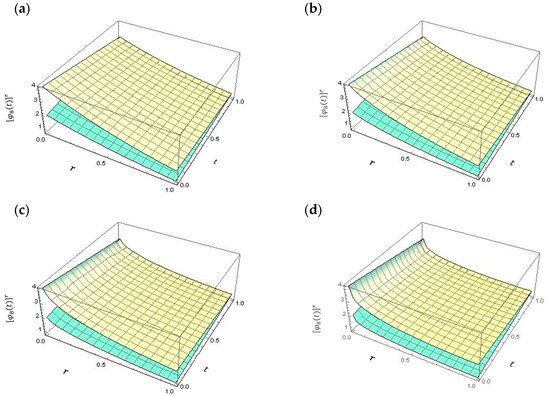
Figure 1. Surface plots of the fuzzy approximated solutions of Example 1, case 1, for all $t\in \left[0,1\right]$, and $r\in \left[0,1\right]$, at various values of $\gamma$: (a) $\gamma =1$; (b) $\gamma =0.85$; (c) $\gamma =0.65$; (d) $\gamma =0.45$: (green and yellow are the lower and the upper solutions, respectively).

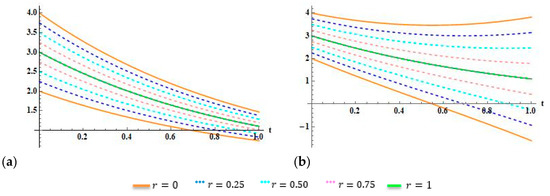
Figure 2. (a) Fuzzy 8th-FS approximated solutions $\left[{\phi }_{8,1r}\left(t\right),{\phi }_{8,2r}\left(t\right)\right]$, case 1. (b) Fuzzy 8th-FS approximated solutions $\left[{\phi }_{8,1r}\left(t\right),{\phi }_{8,2r}\left(t\right)\right]$, case 2, for Example 1 in parametric form, when $\gamma =1$.

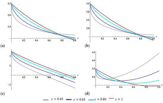
Figure 3. (a) Solution behavior of the Exact and the 8th-FS approximated solutions ${\phi }_{8,1r}\left(t\right)$, case 1; (a,b) Solution behavior of the Exact and the 8th-FS approximated solutions ${\phi }_{8,2r}\left(t\right)$, case 1; (c) Solution behavior of the Exact and the 8th-FS approximated solutions ${\phi }_{8,1r}\left(t\right)$, case 2; (d) Solution behavior of the Exact and the 8th-FS approximated solutions ${\phi }_{8,2r}\left(t\right)$, case 2, for Example 1, when $r=0.5$.

Example 2.

Consider the following FFIVPs:

$$\{\begin{array}{c}{D}_{0^{+}}^{\gamma }\phi \left(t\right)=2t^{\gamma }\phi \left(t\right)+\lambda t^{\gamma },0<\gamma \le 1,t\in \left[0,1\right],\\ \phi \left(0\right)=\mu ,\end{array}$$

(29)

where $\lambda$ and $\mu$ are two fuzzy triangular numbers and have the $r$-level representations $\left[r+1,3-r\right]$.

Indeed, the FFIVPs (29) will be transformed to one of the subsequent systems with respect to type of Caputo differentiability:

Case 1: The system of FIVPs corresponding to Caputo [(1)-$\gamma$]-differentiable is

$$\{\begin{array}{c}{D}_{0^{+}}^{\gamma }{\phi }_{1r}\left(t\right)=2t^{\gamma }{\phi }_{1r}\left(t\right)+\left(r+1\right)t^{\gamma },\\ D_{0^{+}}^{\gamma }{\phi }_{2r}\left(t\right)=2t^{\gamma }{\phi }_{2r}\left(t\right)+\left(3-r\right)t^{\gamma }\\ {\phi }_{1r}\left(0\right)=r+1,{\phi }_{2r}\left(0\right)=3-r.\end{array},$$

(30)

The exact solutions of FIVPs system (30) when $\gamma =1$ could be obtained as

$$\begin{gathered} {\phi }_{1r}\left(t\right)=\frac{1}{2}\left(r+1\right)\left(3e^{t^2}-1\right), \\ {\phi }_{2r}\left(t\right)=\frac{1}{2}\left(3-r\right)\left(3e^{t^2}-1\right). \end{gathered}$$

(31)

In view of the last described FS technique, we took into account ${\phi }_{1r}\left(0\right)={\omega }_0=r+1$ and ${\phi }_{2r}\left(0\right)={\rho }_0=3-r$. Suppose that the $k$-th approximated solutions for FIVPs (30) have the following FS expansions form

$$\begin{gathered} {\phi }_{k,1r}\left(t\right)=\left(r+1\right)+{\displaystyle \sum }_{n=1}^k{\omega }_n\frac{t^{n\gamma }}{\Gamma \left(n\gamma +1\right)}, \\ {\phi }_{k,2r}\left(t\right)=\left(3-r\right)+{\displaystyle \sum }_{n=1}^k{\rho }_n\frac{t^{n\gamma }}{\Gamma \left(n\gamma +1\right)}. \end{gathered}$$

(32)

To determine ${\omega }_n$ and ${\rho }_n,$ $n=1,2,3,\dots ,k,$ we considered the solutions of $D_{0^{+}}^{\left(k-1\right)\gamma }re{s}_{k,1r}\left(0\right)=D_{0^{+}}^{\left(k-1\right)\gamma }re{s}_{k,2r}\left(0\right)=0$, $k=1,2,3,\dots$, in which $re{s}_{k,1r}$ and $re{s}_{k,2r}$ are the $k$th residual functions of (30), defined as

$$\begin{gathered} re{s}_{k,1r}\left(t\right)=D_{0^{+}}^{\gamma }{\phi }_{k,1r}\left(t\right)-2t^{\gamma }{\phi }_{k,1r}\left(t\right)-\left(r+1\right)t^{\gamma }, \\ re{s}_{k,2r}\left(t\right)=D_{0^{+}}^{\gamma }{\phi }_{,k2r}\left(t\right)-2t^{\gamma }{\phi }_{k,2r}\left(t\right)-\left(3-r\right)t^{\gamma }. \end{gathered}$$

(33)

Anyhow, by using the FS algorithm, the first few coefficients ${\omega }_n$ and ${\rho }_n$ are:

$$\begin{array}{c}\hspace{1em}{\omega }_1=0,{\rho }_1=0,\hfill \\ \hspace{1em}{\omega }_2=3\left(r+1\right)\gamma \Gamma \left(\gamma \right),{\rho }_2=3\left(3-r\right)\gamma \Gamma \left(\gamma \right),\hfill \\ \hspace{1em}{\omega }_3=0,{\rho }_3=0,\hfill \\ \hspace{1em}{\omega }_4=\frac{6\left(r+1\right)\gamma \Gamma \left(\gamma \right)\Gamma \left(3\gamma +1\right)}{\Gamma \left(2\gamma +1\right)},{\rho }_4=\frac{6\left(3-r\right)\gamma \Gamma \left(\gamma \right)\Gamma \left(3\gamma +1\right)}{\Gamma \left(2\gamma +1\right)},\hfill \\ \hspace{1em}{\omega }_5=0,{\rho }_5=0,\hfill \\ \hspace{1em}{\omega }_6=\frac{12\left(r+1\right)\gamma \Gamma \left(\gamma \right)\Gamma \left(3\gamma +1\right)\Gamma \left(5\gamma +1\right)}{\Gamma \left(2\gamma +1\right)\Gamma \left(4\gamma +1\right)},\hfill \\ \hspace{1em}{\rho }_6=\frac{12\left(3-r\right)\gamma \Gamma \left(\gamma \right)\Gamma \left(3\gamma +1\right)\Gamma \left(5\gamma +1\right)}{\Gamma \left(2\gamma +1\right)\Gamma \left(4\gamma +1\right)},\hfill \\ ⋮\hfill \\ \mathrm{and}\mathrm{so}\mathrm{on}.\hfill \end{array}$$

Consequently, the 7th-FS approximated solutions of FFIVPs (30) can be represented as

$$\begin{gathered} {\phi }_{7,1r}\left(t\right)=\left(r+1\right)\left(1+\frac{3\gamma \Gamma \left(\gamma \right)t^{2\gamma }}{\Gamma \left(2\gamma +1\right)}+\frac{6\gamma \Gamma \left(\gamma \right)\Gamma \left(3\gamma +1\right)t^{4\gamma }}{\Gamma \left(2\gamma +1\right)\Gamma \left(4\gamma +1\right)}+\frac{12\gamma \Gamma \left(\gamma \right)\Gamma \left(3\gamma +1\right)\Gamma \left(5\gamma +1\right)t^{6\gamma }}{\Gamma \left(2\gamma +1\right)\Gamma \left(4\gamma +1\right)\Gamma \left(6\gamma +1\right)}\right), \\ {\phi }_{7,2r}\left(t\right)=\left(3-r\right)\left(1+\frac{3\gamma \Gamma \left(\gamma \right)t^{2\gamma }}{\Gamma \left(2\gamma +1\right)}+\frac{6\gamma \Gamma \left(\gamma \right)\Gamma \left(3\gamma +1\right)t^{4\gamma }}{\Gamma \left(2\gamma +1\right)\Gamma \left(4\gamma +1\right)}+\frac{12\gamma \Gamma \left(\gamma \right)\Gamma \left(3\gamma +1\right)\Gamma \left(5\gamma +1\right)t^{6\gamma }}{\Gamma \left(2\gamma +1\right)\Gamma \left(4\gamma +1\right)\Gamma \left(6\gamma +1\right)}\right). \end{gathered}$$

For the particular case of $\gamma =1$, the FS-approximated solutions for (30) can be written as

$$\begin{gathered} {\phi }_{1r}\left(t\right)=\underset{k\to \infty }{\lim }{\phi }_{k,1r}\left(t\right)=\left(r-1\right)+\frac{3\left(r-1\right)t^2}{2}+\frac{3\left(r-1\right)t^4}{4}+\frac{3\left(r-1\right)t^6}{12}+\cdots , \\ {\phi }_{2r}\left(t\right)=\underset{k\to \infty }{\lim }{\phi }_{k,2r}\left(t\right)=\left(1-r\right)+\frac{3\left(1-r\right)t^2}{2}+\frac{3\left(1-r\right)t^4}{4}+\frac{3\left(1-r\right)t^6}{12}+\cdots . \end{gathered}$$

and are in agreement with the Taylor series expansions of the exact solutions

$${\phi }_{1r}\left(t\right)=\frac{1}{2}\left(r+1\right)\left(3e^{t^2}-1\right),\mathrm{and}{\phi }_{2r}\left(t\right)=\frac{1}{2}\left(3-r\right)\left(3e^{t^2}-1\right).$$

Case 2:

The system of FIVPs corresponding to Caputo [(2)-$\gamma$]-differentiable is

$$\{\begin{array}{c}{D}_{0^{+}}^{\gamma }{\phi }_{1r}\left(t\right)=2t^{\gamma }{\phi }_{2r}\left(t\right)+\left(3-r\right)t^{\gamma },\\ D_{0^{+}}^{\gamma }{\phi }_{2r}\left(t\right)=2t^{\gamma }{\phi }_{1r}\left(t\right)+\left(r+1\right)t^{\gamma },\\ {\phi }_{1r}\left(0\right)=r+1,{\phi }_{2r}\left(0\right)=3-r.\end{array}$$

(34)

The exact solutions of FIVPs system (34) when $\gamma =1$ could be obtained as

$$\begin{gathered} {\phi }_{1r}\left(t\right)=-\frac{1}{2}\left(1+r\right)+3e^{t^2}+\frac{1}{2}\left(r-1\right)e^{-t^2}, \\ {\phi }_{2r}\left(t\right)=-\frac{1}{2}\left(3-r\right)+3e^{t^2}+\frac{1}{2}\left(1-r\right)e^{-t^2}. \end{gathered}$$

(35)

According to the application of the RPS approach, selecting ${\phi }_{1r}\left(0\right)=r-1$ and ${\phi }_{2r}\left(0\right)=1-r$, we obtained the 0th-FS approximated solutions; then, the $k$^th-truncated FS approximated solutions for FIVPs (34) are given by the following forms:

$$\begin{gathered} {\phi }_{k,1r}\left(t\right)=\left(r+1\right)+{\displaystyle \sum }_{n=1}^k{\omega }_n\frac{t^{n\gamma }}{\Gamma \left(n\gamma +1\right)}, \\ {\phi }_{k,2r}\left(t\right)=\left(3-r\right)+{\displaystyle \sum }_{n=1}^k{\rho }_n\frac{t^{n\gamma }}{\Gamma \left(n\gamma +1\right)}. \end{gathered}$$

(36)

Next, we defined the $k$th-residual functions $re{s}_{k,1r}$ and $re{s}_{k,2r}$ for (34) as follows:

$$\begin{gathered} re{s}_{k,1r}\left(t\right)=D_{0^{+}}^{\gamma }\left(\left(r+1\right)+{\displaystyle \sum }_{n=1}^k{\omega }_n\frac{t^{n\gamma }}{\Gamma \left(n\gamma +1\right)}\right)-2t^{\gamma }\left(\left(3-r\right)+{\displaystyle \sum }_{n=1}^k{\rho }_n\frac{t^{n\gamma }}{\Gamma \left(n\gamma +1\right)}\right)-\left(3-r\right)t^{\gamma }, \\ re{s}_{k,2r}\left(t\right)=D_{0^{+}}^{\gamma }\left(\left(3-r\right)+{\displaystyle \sum }_{n=1}^k{\rho }_n\frac{t^{n\gamma }}{\Gamma \left(n\gamma +1\right)}\right)-2t^{\gamma }\left(\left(r+1\right)+{\displaystyle \sum }_{n=1}^k{\omega }_n\frac{t^{n\gamma }}{\Gamma \left(n\gamma +1\right)}\right)-\left(r+1\right)t^{\gamma }. \end{gathered}$$

(37)

Following the procedure of the RPS algorithm, the first few coefficients ${\omega }_n$ and ${\rho }_n$ are

$$\begin{array}{c}{\omega }_1=0,{\rho }_1=0,\hfill \\ {\omega }_2=3\left(3-r\right)\gamma \Gamma \left(\gamma \right),{\rho }_2=3\left(1+r\right)\gamma \Gamma \left(\gamma \right),\hfill \\ {\omega }_3=0,{\rho }_3=0,\hfill \\ {\omega }_4=\frac{6\left(1+r\right)\gamma \Gamma \left(\gamma \right)\Gamma \left(3\gamma +1\right)}{\Gamma \left(2\gamma +1\right)},{\rho }_4=\frac{6\left(3-r\right)\gamma \Gamma \left(\gamma \right)\Gamma \left(3\gamma +1\right)}{\Gamma \left(2\gamma +1\right)},\hfill \\ {\omega }_5=0,{\rho }_5=0,\hfill \\ {\omega }_6=\frac{12\left(3-r\right)\gamma \Gamma \left(\gamma \right)\Gamma \left(3\gamma +1\right)\Gamma \left(5\gamma +1\right)}{\Gamma \left(2\gamma +1\right)\Gamma \left(4\gamma +1\right)},{\rho }_6=\frac{12\left(1+r\right)\gamma \Gamma \left(\gamma \right)\Gamma \left(3\gamma +1\right)\Gamma \left(5\gamma +1\right)}{\Gamma \left(2\gamma +1\right)\Gamma \left(4\gamma +1\right)},\hfill \\ {\omega }_7=0,{\rho }_7=0,\hfill \\ {\omega }_8=\frac{24\left(1+r\right)\gamma \Gamma \left(\gamma \right)\Gamma \left(3\gamma +1\right)\Gamma \left(5\gamma +1\right)\Gamma \left(7\gamma +1\right)}{\Gamma \left(2\gamma +1\right)\Gamma \left(4\gamma +1\right)\Gamma \left(6\gamma +1\right)},\hfill \\ {\rho }_8=\frac{24\left(3-r\right)\gamma \Gamma \left(\gamma \right)\Gamma \left(3\gamma +1\right)\Gamma \left(5\gamma +1\right)\Gamma \left(7\gamma +1\right)}{\Gamma \left(2\gamma +1\right)\Gamma \left(4\gamma +1\right)\Gamma \left(6\gamma +1\right)},\hfill \\ \hfill ⋮\hfill \\ \mathrm{and}\mathrm{so}\mathrm{on}.\hfill \end{array}$$

Therefore, the 8th-FS approximated solutions of FIVPs (34) can be represented as

$$\begin{gathered} {\phi }_{8,1r}\left(t\right)=\left(r+1\right)+\frac{3\gamma \Gamma \left(\gamma \right)t^{2\gamma }}{\Gamma \left(2\gamma +1\right)}\left(3-r+\frac{2t^{2\gamma }\Gamma \left(3\gamma +1\right)}{\Gamma \left(4\gamma +1\right)\Gamma \left(6\gamma +1\right)\Gamma \left(8\gamma +1\right)}\left(\left(1+r\right)\Gamma \left(6\gamma +1\right)\Gamma \left(8\gamma +1\right)+2t^{2\gamma }\Gamma \left(5\gamma +1\right)\left(2\left(1+r\right)t^{2\gamma }\Gamma \left(7\gamma +1\right)+\left(3-r\right)\Gamma \left(8\gamma +1\right)\right)\right)\right), \\ {\phi }_{8,2r}\left(t\right)=\left(3-r\right)+\frac{3\gamma \Gamma \left(\gamma \right)t^{2\gamma }}{\Gamma \left(2\gamma +1\right)}\left(1+r+\frac{2t^{2\gamma }\Gamma \left(3\gamma +1\right)}{\Gamma \left(4\gamma +1\right)\Gamma \left(6\gamma +1\right)\Gamma \left(8\gamma +1\right)}\left(\left(3-r\right)\Gamma \left(6\gamma +1\right)\Gamma \left(8\gamma +1\right)+2t^{2\gamma }\Gamma \left(5\gamma +1\right)\left(2\left(3-r\right)t^{2\gamma }\Gamma \left(7\gamma +1\right)+\left(1+r\right)\Gamma \left(8\gamma +1\right)\right)\right)\right). \end{gathered}$$

(38)

Correspondingly, for $\gamma =1$, the 8th-FS approximated solutions (38) can be written as

$$\begin{gathered} {\phi }_{8,1r}\left(t\right)=\left(1+r\right)+\frac{3}{2}{t}^2\left(3-r+\frac{t^2\left(29030400\left(1+r\right)+240t^2\left(40320\left(3-r\right)+10080\left(1+r\right)t^2\right)\right)}{58060800}\right), \\ {\phi }_{8,2r}\left(t\right)=\left(3-r\right)+\frac{3}{2}{t}^2\left(1+r+\frac{t^2\left(29030400\left(3-r\right)+240t^2\left(40320\left(1+r\right)-10080\left(-3+r\right)t^2\right)\right)}{58060800}\right). \end{gathered}$$

(39)

which agrees with the first eighth terms of the MacLaurin series of the exact forms ${\phi }_{1r}\left(t\right)=-\frac{1}{2}\left(1+r\right)+3e^{t^2}+\frac{1}{2}\left(r-1\right)e^{-t^2}$, and ${\phi }_{2r}\left(t\right)=-\frac{1}{2}\left(3-r\right)+3e^{t^2}+\frac{1}{2}\left(1-r\right)e^{-t^2}$.

Table 4 presents the absolute errors of the obtained solutions by the RPS method for Example 2, case 2. The results in Table 4 show that the absolute errors of the proposed method were quite small. Further, numerical simulations of the outcomes for Example 2, case 1, were performed and are presented in Table 5.

Table 4. Absolute errors of Example 2, case 2, at $n=8$ and various $r$ values.

	${\mathit{t}}_{\mathit{i}}$	$\mathit{r}=0.25$	$\mathit{r}=0.5$	$\mathit{r}=0.75$	$\mathit{r}=1$
${\phi }_{1r}\left(t\right)$	$0.16$	$4.000000\times {10}^{-10}$	$4.000000\times {10}^{-10}$	$4.000000\times {10}^{-10}$	$2.000000\times {10}^{-10}$
	$0.36$	$1.269000\times {10}^{-6}$	$1.158000\times {10}^{-6}$	$1.046000\times {10}^{-6}$	$9.340000\times {10}^{-7}$
	$0.56$	$1.069870\times {10}^{-4}$	$9.798300\times {10}^{-4}$	$8.897900\times {10}^{-5}$	$7.997400\times {10}^{-5}$
	$0.76$	$2.324840\times {10}^{-3}$	$2.141800\times {10}^{-3}$	$1.958750\times {10}^{-3}$	$1.775700\times {10}^{-3}$
	$0.96$	$2.494130\times {10}^{-2}$	$2.314519\times {10}^{-2}$	$2.134908\times {10}^{-2}$	$1.955297\times {10}^{-2}$
${\phi }_{2r}\left(t\right)$	$0.16$	$2.000000\times {10}^{-10}$	$3.000000\times {10}^{-10}$	$2.000000\times {10}^{-10}$	$2.000000\times {10}^{-10}$
	$0.36$	$5.980000\times {10}^{-7}$	$7.100000\times {10}^{-7}$	$8.220000\times {10}^{-7}$	$9.340000\times {10}^{-7}$
	$0.56$	$5.296200\times {10}^{-5}$	$6.196600\times {10}^{-5}$	$7.097000\times {10}^{-5}$	$7.997400\times {10}^{-5}$
	$0.76$	$1.226540\times {10}^{-3}$	$1.409600\times {10}^{-3}$	$1.592650\times {10}^{-3}$	$1.775700\times {10}^{-3}$
	$0.96$	$1.416464\times {10}^{-2}$	$1.596075\times {10}^{-2}$	$1.775686\times {10}^{-2}$	$1.955297\times {10}^{-2}$

Table 5. Numerical results of the fuzzy 8th-FS approximated solutions $\left[{\phi }_{8,1r}\left(t\right),{\phi }_{8,2r}\left(t\right)\right]$ with various values of $\gamma$ and $r$ for Example 2, case 1.

${\mathit{\gamma }}_{\mathit{i}}$	${\mathit{t}}_{\mathit{i}}$	$\mathit{r}=0.2$	$\mathit{r}=0.6$	$\mathit{r}=1.0$
$1$	$0.15$	$\left[1.2409590,2.8955710\right]$	$\left[1.6546121,2.4819181\right]$	$\left[2.0682651,2.0682651\right]$
	$0.30$	$\left[1.3695087,3.1955203\right]$	$\left[1.8260116,2.7390174\right]$	$\left[2.2825145,2.2825145\right]$
	$0.45$	$\left[1.6038968,3.7424258\right]$	$\left[2.1385291,3.2077935\right]$	$\left[2.6731612,2.6731612\right]$
	$0.60$	$\left[1.9786368,4.6168192\right]$	$\left[2.6381824,3.9572736\right]$	$\left[3.2977280,3.2977280\right]$
$0.85$	$0.15$	$\left[1.2900668,3.0101558\right]$	$\left[1.7200890,2.5801335\right]$	$\left[2.1501113,2.1501113\right]$
	$0.30$	$\left[1.5117406,3.5273948\right]$	$\left[2.0156542,3.0234813\right]$	$\left[2.5195677,2.519567\right]$
	$0.45$	$\left[1.8810863,4.3892014\right]$	$\left[2.5081151,3.7621726\right]$	$\left[3.1351438,3.1351438\right]$
	$0.60$	$\left[2.4495733,5.7156709\right]$	$\left[3.2660977,4.8991466\right]$	$\left[4.0826221,4.0826221\right]$
$0.65$	$0.15$	$\left[1.4577914,3.4015132\right]$	$\left[1.9437218,2.9155827\right]$	$\left[2.4296523,2.4296523\right]$
	$0.30$	$\left[1.9263358,4.4947835\right]$	$\left[2.5684477,3.8526716\right]$	$\left[3.2105596,3.2105596\right]$
	$0.45$	$\left[2.6433967,6.1679256\right]$	$\left[3.5245289,5.2867934\right]$	$\left[4.4056612,4.4056612\right]$
	$0.60$	$\left[3.6985342,8.6299130\right]$	$\left[4.9313789,7.3970683\right]$	$\left[6.1642236,6.1642236\right]$

Next, the numerical comparisons of the errors for Example 2 under Caputo [(1)-$\gamma$]-differentiability are discussed using our method and the homotopy analysis (HA) method [41] for different values of $r$, as shown in Table 6. From this table, one can observe that the RPS solutions were more accurate than the HA solutions.

Table 6. Numerical comparison of the approximated solutions of Example 2, case 1, at $t=1$ and different values of $r$.

${\mathit{r}}_{\mathit{i}}$	$\mathbf{Absolute}\mathbf{Errors}\mathbf{of}{\mathit{\phi }}_{1\mathit{r}}\left(\mathit{t}\right)$
	RPS method	HA method
$0$	$4.09689\times {10}^{-8}$	$4.09689\times {10}^{-5}$
$0.2$	$3.20000\times {10}^{-8}$	$3.34322\times {10}^{-5}$
$0.4$	$2.40000\times {10}^{-8}$	$2.50742\times {10}^{-5}$
$0.6$	$1.60000\times {10}^{-8}$	$1.67161\times {10}^{-5}$
$0.8$	$8.0000\times {10}^{-9}$	$8.35806\times {10}^{-6}$
$1$	$0.0$	$0.0$
${\mathit{r}}_{\mathit{i}}$	$\mathbf{Absolute}\mathbf{Errors}\mathbf{of}{\mathit{\phi }}_{1\mathit{r}}\left(\mathit{t}\right)$
	RPS method	HA method
$0$	$4.09689\times {10}^{-8}$	$3.34475\times {10}^{-5}$
$0.2$	$3.20000\times {10}^{-8}$	$2.67580\times {10}^{-5}$
$0.4$	$2.40000\times {10}^{-8}$	$2.00685\times {10}^{-5}$
$0.6$	$1.60000\times {10}^{-8}$	$1.33790\times {10}^{-5}$
$0.8$	$8.00000\times {10}^{-9}$	$6.68949\times {10}^{-6}$
$1$	$0.0$	$0.0$

The surface plots in Figure 4 show the 8th-FS approximated solution behavior at various values of $\gamma$ for $\left(t,r\right)\in {\left[0,1\right]}^2$, for Example 2, case 2. Figure 5 illustrates the effect of the parameter $r$ on the obtained solutions against the exact solutions for Example 2, case 2, at standard order $\gamma =1$.

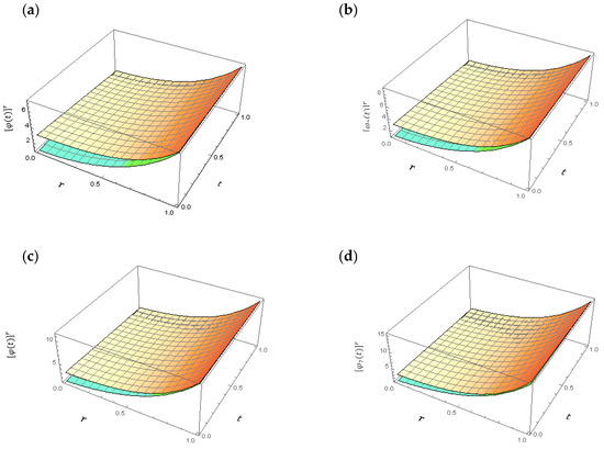
Figure 4. Surface plot of the fuzzy 7th-FS approximated solutions, of Example 2, case 2, for all $t\in \left[0,1\right]$ and $r\in \left[0,1\right]$ at various values of $\gamma$: (a) $\gamma =1$; (b) $\gamma =0.9$; (c) $\gamma =0.8$; (d) $\gamma =0.7$; (green and yellow are the lower and the upper solutions, respectively).

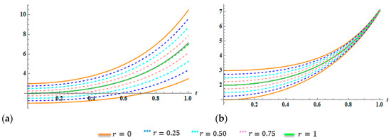
Figure 5. (a) Fuzzy approximated solutions $\left[{\phi }_{7,1r}\left(t\right),{\phi }_{7,2r}\left(t\right)\right]$, case 1. (b) Fuzzy approximated solutions $\left[{\phi }_{8,1r}\left(t\right),{\phi }_{8,2r}\left(t\right)\right]$, case 2, for Example 2, in parametric form, when $\gamma =1$.

6. Conclusions

The major aim of the current analysis was to propose an efficient approach for obtaining fuzzy approximated solutions of FFIVPs with the assumption of strongly generalized differentiability. The main equations can be reformulated in parametric form and then translated into a fractional IVPs system to be solved by the RPS approach. This approach was applied directly by choosing suitable uncertain initial data to construct approximated solutions in the FS expansion with no need for nonphysical restrictive hypotheses. Numerical examples were provided to clarify the compatibility and reliability of the RPS approach. The graphical and numerical results satisfied the convex symmetric triangular fuzzy number and indicated that the proposed approach is an accurate instrument that can be used suitably as an alternative approach for constructing analytical solutions of diverse kinds of fuzzy fractional problems appearing in the fields of physics and engineering. In future work, it will be possible to apply the proposed approach for solving coupled systems of FFIVPs, fuzzy fractional BVPs with different order of $\gamma$, and fuzzy delay models.

References

- Caputo, M. Linear models of dissipation whose Q is almost frequency independent: Part II. Geophys. J. Int. 1967, 13, 529–539. [Google Scholar] [CrossRef]
- Momani, S.; Freihat, A.; Al-Smadi, M. Analytical study of fractional-order multiple chaotic Fitzhugh-Nagumo neurons model using multistep generalized differential transform method. Abstr. Appl. Anal. 2014, 2014, 276279. [Google Scholar] [CrossRef] [PubMed] [Green Version]
- Al-Smadi, M.; Abu Arqub, O. Computational algorithm for solving fredholm time-fractional partial integrodifferential equations of dirichlet functions type with error estimates. Appl. Math. Comput. 2019, 342, 280–294. [Google Scholar] [CrossRef]
- Altawallbeh, Z.; Al-Smadi, M.; Komashynska, I.; Ateiwi, A. Numerical solutions of fractional systems of two-point BVPs by using the iterative reproducing kernel algorithm. Ukr. Math. J. 2018, 70, 687–701. [Google Scholar] [CrossRef]
- Alabedalhadi, M.; Al-Smadi, M.; Al-Omari, S.; Baleanu, D.; Momani, S. Structure of optical soliton solution for nonliear resonant space-time Schrödinger equation in conformable sense with full nonlinearity term. Phys. Scr. 2020, 95, 105215. [Google Scholar] [CrossRef]
- Al-Smadi, M.; Abu Arqub, O.; Gaith, M. Numerical simulation of telegraph and Cattaneo fractional-type models using adaptive reproducing kernel framework. Math. Methods Appl. Sci. 2021, 44, 8472–8489. [Google Scholar] [CrossRef]
- Agarwal, R.P.; Lakshmikantham, V.; Nieto, J.J. On the concept of solution for fractional differential equations with uncertainty. Nonlinear Anal. Theory Methods Appl. 2010, 72, 2859–2862. [Google Scholar] [CrossRef]
- Al-Smadi, M.; Abu Arqub, O.; Zeidan, D. Fuzzy fractional differential equations under the Mittag-Leffler kernel differential operator of the ABC approach: Theorems and applications. Chaos Solitons Fractals 2021, 146, 110891. [Google Scholar] [CrossRef]
- Ahmadian, A.; Suleiman, M.; Salahshour, S.; Baleanu, D. A Jacobi operational matrix for solving a fuzzy linear fractional differential equation. Adv. Differ. Equ. 2013, 2013, 104–115. [Google Scholar] [CrossRef] [Green Version]
- Jafarian, A.; Golmankhaneh, A.K.; Baleanu, D. On fuzzy fractional Laplace transformation. Adv. Math. Phys. 2014, 2014, 295432. [Google Scholar] [CrossRef]
- Hasan, S.; Al-Smadi, M.; El-Ajou, A.; Momani, S.; Hadid, S.; Al-Zhour, Z. Numerical approach in the Hilbert space to solve a fuzzy Atangana-Baleanu fractional hybrid system. Chaos Solitons Fractals 2021, 143, 110506. [Google Scholar] [CrossRef]
- Al-Smadi, M.; Dutta, H.; Hasan, S.; Momani, S. On numerical approximation of Atangana-Baleanu-Caputo fractional integro-differential equations under uncertainty in Hilbert Space. Math. Model. Nat. Phenom. 2021, 16, 41. [Google Scholar] [CrossRef]
- Harrouche, N.; Momani, S.; Hasan, S.; Al-Smadi, M. Computational algorithm for solving drug pharmacokinetic model under uncertainty with nonsingular kernel type Caputo-Fabrizio fractional derivative. Alex. Eng. J. 2021, 60, 4347–4362. [Google Scholar] [CrossRef]
- Arshad, S.; Lupulescu, V. On the fractional differential equations with uncertainty. Nonlinear Anal. 2011, 74, 3685–3693. [Google Scholar] [CrossRef]
- Alikhani, R.; Bahrami, F. Global solutions for nonlinear fuzzy fractional integral and integrodifferential equations. Commun. Nonlinear Sci. Numer. Simul. 2013, 18, 2007–2017. [Google Scholar] [CrossRef]
- Mazandarani, M.; Najariyan, M. Type-2 fuzzy fractional derivatives. Commun. Nonlinear Sci. Numer. Simul. 2014, 19, 2354–2372. [Google Scholar] [CrossRef]
- Salahshour, S.; Allahviranloo, T.; Abbasbandy, S.; Baleanu, D. Existence and uniqueness results for fractional differential equations with uncertainty. Adv. Diff. Equ. 2012, 2012, 112. [Google Scholar] [CrossRef] [Green Version]
- Alaroud, M.; Al-Smadi, M.; Ahmad, R.R.; Salma Din, U.K. Computational optimization of residual power series algorithm for certain classes of fuzzy fractional differential equations. Int. J. Differ. Equ. 2018, 2018, 8686502. [Google Scholar] [CrossRef]
- Alaroud, M.; Al-Smadi, M.; Rozita Ahmad, R.; Salma Din, U.K. An analytical numerical method for solving fuzzy fractional Volterra integro-differential equations. Symmetry 2019, 11, 205. [Google Scholar] [CrossRef] [Green Version]
- Gumah, G.; Naser, M.F.M.; Al-Smadi, M.; Al-Omari, S.K.Q.; Baleanu, D. Numerical solutions of hybrid fuzzy differential equations in a Hilbert space. Appl. Numer. Math. 2020, 151, 402–412. [Google Scholar] [CrossRef]
- Alshammari, M.; Al-Smadi, M.; Abu Arqub, O.; Hashim, I.; Alias, M.A. Residual series representation algorithm for solving fuzzy duffing oscillator equations. Symmetry 2020, 12, 572. [Google Scholar] [CrossRef] [Green Version]
- Bede, B.; Gal, S.G. Generalizations of the differentiability of fuzzy number value functions with applications to fuzzy differential equations. Fuzzy Sets Syst. 2005, 151, 581–599. [Google Scholar] [CrossRef]
- Chalco-Cano, Y.; Román-Flores, H. On new solutions of fuzzy differential equations. Chaos Solitons Fractals 2008, 38, 112–119. [Google Scholar] [CrossRef]
- Kaleva, O. Fuzzy differential equations. Fuzzy Sets Syst. 1987, 24, 301–317. [Google Scholar] [CrossRef]
- Abu Arqub, O. Series solution of fuzzy differential equations under strongly generalized differentiability. J. Adv. Res. Appl. Math. 2013, 5, 31–52. [Google Scholar] [CrossRef]
- Al-Smadi, M.; Abu Arqub, O.; Hadid, S. Approximate solutions of nonlinear fractional Kundu-Eckhaus and coupled fractional massive Thirring equations emerging in quantum field theory using conformable residual power series method. Phys. Scr. 2020, 95, 10520. [Google Scholar] [CrossRef]
- Al-Smadi, M.; Abu Arqub, O.; Hadid, S. An attractive analytical technique for coupled system of fractional partial differential equations in shallow water waves with conformable derivative. Commun. Theor. Phys. 2020, 72, 085001. [Google Scholar] [CrossRef]
- Al-Smadi, M.; Abu Arqub, O.; Momani, S. Numerical computations of coupled fractional resonant Schrödinger equations arising in quantum mechanics under conformable fractional derivative sense. Phys. Scr. 2020, 95, 075218. [Google Scholar] [CrossRef]
- El-Ajou, A.; Abu Arqub, O.; Al-Smadi, M. A general form of the generalized Taylor’s formula with some applications. Appl. Math. Comput. 2015, 256, 851–859. [Google Scholar] [CrossRef]
- Hasan, S.; Djeddi, N.; Al-Smadi, M.; Al-Omari, S.; Momani, S.; Pulga, A. Numerical solvability of generalized Bagley-Torvik fractional models under Caputo-Fabrizio derivative. Adv. Differ. Equ. 2021, 2021, 469. [Google Scholar] [CrossRef]
- Hasan, S.; Al-Smadi, M.; Freihet, A.; Momani, S. Two computational approaches for solving a fractional obstacle system in Hilbert space. Adv. Differ. Equ. 2019, 2019, 55. [Google Scholar] [CrossRef] [Green Version]
- Abu-Gaairi, R.; Hasan, S.; Al-Omari, S.; Al-Smadi, M.; Momani, S. Attractive multistep reproducing kernel approach for solving stiffness differential systems of ordinary differential equations and some error analysis. Compu. Model. Eng. Sci. 2022, 130, 299–313. [Google Scholar]
- Freihet, A.; Hasan, S.; Al-Smadi, M.; Gaith, M.; Momani, S. Construction of fractional power series solutions to fractional stiff system using residual functions algorithm. Adv. Differ. Equ. 2019, 2019, 95. [Google Scholar] [CrossRef] [Green Version]
- Freihet, A.; Hasan, S.; Alaroud, M.; Al-Smadi, M.; Ahmad, R.R.; Salma Din, U.K. Toward computational algorithm for time-fractional Fokker–Planck models. Adv. Mech. Eng. 2019, 11, 1687814019881039. [Google Scholar] [CrossRef]
- Al-Smadi, M.; Djeddi, N.; Momani, S.; Al-Omari, S.; Araci, S. An attractive numerical algorithm for solving nonlinear Caputo–Fabrizio fractional Abel differential equation in a Hilbert space. Adv. Differ. Equ. 2021, 2021, 271. [Google Scholar] [CrossRef]
- Moaddy, K.; Al-Smadi, M.; Hashim, I. A novel representation of the exact solution for differential algebraic equations system using residual power-series method. Discret. Dyn. Nat. Soc. 2015, 2015, 205207. [Google Scholar] [CrossRef]
- Saadeh, R.; Alaroud, M.; Al-Smadi, M.; Ahmad, R.R.; Salma Din, U.K. Application of fractional residual power series algorithm to solve Newell–Whitehead–Segel equation of fractional order. Symmetry 2019, 11, 1431. [Google Scholar] [CrossRef] [Green Version]
- Hasan, S.; Al-Smadi, M.; Dutta, H.; Momani, S.; Hadid, S. Multi-step reproducing kernel algorithm for solving Caputo–Fabrizio fractional stiff models arising in electric circuits. Soft Comput. 2022, 26, 3713–3727. [Google Scholar] [CrossRef]
- Aljarrah, H.; Alaroud, M.; Ishak, A.; Darus, M. Adaptation of residual-error series algorithm to handle fractional system of partial differential equations. Mathematics 2021, 9, 2868. [Google Scholar] [CrossRef]
- Allahviranloo, T.; Noeiaghdam, Z.; Noeiaghdam, S.; Nieto, J.J. A fuzzy method for solving fuzzy fractional differential equations based on the generalized fuzzy taylor expansion. Mathematics 2020, 8, 2166. [Google Scholar] [CrossRef]
- Abu Arqub, O.; Abo-Hammour, Z.; Al-Badarneh, R.; Momani, S. A reliable analytical method for solving higher-order initial value problems. Discret. Dyn. Nat. Soc. 2013, 2013, 673829. [Google Scholar] [CrossRef]
Publisher’s Note: MDPI stays neutral with regard to jurisdictional claims in published maps and institutional affiliations. |
© 2022 by the authors. Licensee MDPI, Basel, Switzerland. This article is an open access article distributed under the terms and conditions of the Creative Commons Attribution (CC BY) license (https://creativecommons.org/licenses/by/4.0/).