Article

Coupled Fixed Points for Hardy–Rogers Type of Maps and Their Applications in the Investigations of Market Equilibrium in Duopoly Markets for Non-Differentiable, Nonlinear Response Functions

by
Stanimir Kabaivanov
1,*,
Vasil Zhelinski
2 and
Boyan Zlatanov
2,*
1
Faculty of Economics and Social Sciences, University of Plovdiv Paisii Hilendarski, 4000 Plovdiv, Bulgaria
2
Faculty of Mathematics and Informatics, University of Plovdiv Paisii Hilendarski, 4000 Plovdiv, Bulgaria
*
Authors to whom correspondence should be addressed.
Symmetry 2022, 14(3), 605; https://doi.org/10.3390/sym14030605
Submission received: 13 February 2022 / Revised: 8 March 2022 / Accepted: 15 March 2022 / Published: 18 March 2022
(This article belongs to the Section Mathematics)

Abstract

:
In this paper we generalize Hardy–Rogers maps in the context of coupled fixed points. We comment on the symmetry of some of the coefficients involved in the Hardy–Rogers condition, and thus, we deduce a simpler formula. We generalize, with the help of the obtained main theorem, some known results about existence and uniqueness of market equilibrium in duopoly markets. As a consequence, we ascertain that the equilibrium production should be equal for both market participants provided that they have symmetric response functions. With the help of the main theorem, we investigate and enrich some recent results regarding market equilibrium in duopoly markets. We define a generalized response function that includes production and surpluses. Finally, we illustrate a possible application of the main result in the investigation of market equilibrium when the payoff functions are non-differentiable.
MSC:
46B07; 46B20; 46B25; 55M20
JEL Classification:
C02; D43; C62

1. Introduction

The investigation of coupled fixed points started in 1987 from the article [1]. The first result [1] deals with maps with the mixed monotone property in complete, partially ordered metric spaces. There are a great number of contemporary research papers on the theory of coupled fixed points with the mixed monotone property [2], without the mixed monotone property [3], in ordered probabilistic metric spaces [4], in modular metric spaces [5], in metric spaces endowed with a graph [6], fuzzy cone metric spaces [7], in b-metric spaces [8], and for multi-valued maps [9]. The idea of coupled fixed points was generalized for coupled best-proximity points [10]. There are applications of coupled fixed points in different fields of mathematics—impulsive differential equations [6], integral equations [11], ordinary differential equations [12], periodic boundary value problems [13], fractional equations [14], and nonlinear matrix equations [15]—and in other sciences—economics [16,17], aquatic ecosystems [18], and dynamic programming [19]—with these just being the most recent investigations dealing with coupled fixed points.
Important results about the connection between coupled fixed points and fixed points are obtained in [20]. Following the technique suggested in [20], we present a generalization of Hardy–Rogers maps in the coupled fixed point theory. It has been noticed and proven in [16] that whenever the functions F i : X 1 × X 2 X i , i = 1 , 2 , involved in the model, satisfy a symmetric condition, i.e., F 2 ( x , y ) = F 1 ( y , x ) , then the coupled fixed points ( ξ , η ) should satisfy ξ = η . This result can be used to study a lot of different economic processes, and we utilize it in studying markets with few dominant players. If we take out the extreme case of a single participant, the simplest example would be a case with only two players: a duopoly market.
The analysis of market equilibrium in duopoly markets was pioneered by [21] in 1897. Due to its practical importance, it is still a matter of high interest and rapid development nowadays [22,23]. The classical approach is to maximize the payoff function of the two participants in the market [24,25,26] with the justification that rational players will always try to gain maximum profitability in the real world. Modern businesses are managed and evaluated against several key performance indicators (KPIs), including new product development, gain of market share, and consumer satisfaction. These factors do not exclude the pursuit of profits, but the focus is more biased toward long-term gains and performance. Therefore, a different approach has been suggested in [16] by considering the response functions of both players rather than maximizing their payoffs. While current-period profits are important, management practices that aim solely at their maximization may not provide the best foundation for long-term growth and market dominance. Thus, focusing solely on the short-term gains cannot explain actions of duopoly market players in contemporary global markets. Similar to real-world travel, there are several ways to reach a destination. The complexity and size of contemporary business organizations varies and is the basis upon which they choose the most suitable path. Yet such options offer different short-term strategies, despite being universally oriented toward long-term success. An example of different sub-goals that support expansion could be policies that boost workforce engagement or actions oriented toward takeovers to add new customers and resources. Quite often we face a combination of sub-goals in a company’s strategic plans. With various master plans, business entities will respond differently to economic changes. For an outsider these could look like sub-optimal solutions, but they may be well-aligned with the long-term company strategy. Even in markets with very few competitors, substitution of goods and globalization have driven a change toward introducing specialized products and non-homogeneous outputs. This is a very special deviation from early models, where homogeneous goods were assumed to be supplied. While one can argue that there are a lot of situations where the outputs may be virtually identical (for example, the case of raw materials), a sound market model should also be able to explain situations where products are different. In such cases, companies face a large number of opportunities to gain competitive advantage—in particular ones that are not based on price. Differences in organizational structure impose another challenge for traditional models. In particular, complexity in decision-making processes can result in increases of the time required to decide on and implement an action. Therefore, the assumption that price changes can happen immediately and with the same pace for each player is too restrictive and not realistic. Some decisions require more time than others. In the extreme case, they may even be considered unfeasible due to technological or scale concerns (for example, change in production levels may not be possible due to batch processing, minimum number of outputs, or technological concerns that produce a discrete number of products at once). Thus, the real-world outputs are not perfectly divisible. This fact imposes an additional restriction on how companies react and behave in duopoly markets. Recent developments as a result of the COVID-19 crisis and shortages of some crucial components have proven to be a very significant test on how companies can react in nonlinear way. In particular, the need to change production output dramatically due to quick price jumps offers a possibility to test our suggestions and highlights the benefits of the model, as discussed below.
We have tried to generalize these ideas by showing that the maximization problem may lack the second order conditions, due to a nondifferentiabilty of the payoff functions.

2. Materials and Methods

Definition 1
([27]). Let ( X , ρ ) be a metric space. A map T : X X is a Hardy–Rogers map if there are non-negative constants a i , i = 1 , 2 , 3 , 4 , 5 , satisfying i = 1 5 a i < 1 , so that for any x , y X holds the inequality:
ρ ( T x , T y ) a 1 ρ ( x , y ) + a 2 ρ ( x , T x ) + a 3 ρ ( y , T y ) + a 4 ρ ( x , T y ) + a 5 ρ ( y , T x ) .
As pointed out in [28], from the symmetry of the metric function ρ ( · , · ) it follows that if (1) holds true then there will hold the inequality:
ρ ( T x , T y ) a 1 ρ ( x , y ) + a 2 + a 3 2 ( ρ ( x , T x ) + ρ ( y , T y ) ) + a 4 + a 5 2 ( ρ ( x , T y ) + ρ ( y , T x ) ) .
Therefore, without loss of generality we can consider maps that satisfy the inequality:
ρ ( T x , T y ) k 1 ρ ( x , y ) + k 2 ( ρ ( x , T x ) + ρ ( y , T y ) ) + k 3 ( ρ ( x , T y ) + ρ ( y , T x ) ) ,
so that k 1 + 2 k 2 + 2 k 3 < 1 .
If k 2 = k 3 = 0 we get a Banach contraction map, if k 1 = k 3 = 0 we get a Kannan contraction map [29], and if k 1 = k 2 = 0 we get a Chatterjea contraction map [30].
In what follows, we will assume that a Hardy–Rogers maps satisfies (2).
Theorem 1
([28]). Let ( X , ρ ) be a complete metric space and T : X X be a Hardy–Rogers map, then:
1. 
there is a unique fixed point ξ X of T and, moreover, for any initial guess x 0 X , the iterated sequence x n = T x n 1 for n = 1 , 2 , converges to the fixed point ξ;
2. 
there holds a priori error estimates ρ ( ξ , x n ) k n 1 k ρ ( x 0 , x 1 ) ;
3. 
there holds a posteriori error estimate ρ ( ξ , x n ) k 1 k ρ ( x n 1 , x n ) ;
4. 
the rate of convergence is ρ ( ξ , x n ) k ρ ( ξ , x n 1 ) ;
where k = k 1 + k 2 + k 3 1 k 2 k 3 and k i = 1 , 2 , 3 are the constants from (2).
Definition 2
([1]). Let A be nonempty subset of a metric space ( X , ρ ) , F : A × A A . An ordered pair ( ξ , η ) A × A is called a coupled fixed point of F in A if ξ = F ( ξ , η ) and η = F ( η , ξ ) .
A generalization of the above-mentioned notions was presented in order to apply the technique of coupled fixed points in the investigation of market equilibrium [16]. In duopoly markets, naturally each of the players has a different response reaction based on its rival and the market. Thus, two response functions F i for i = 1 , 2 were considered in [16], such that F i : X 1 × X 2 X i , i = 1 , 2 , where X i is the production set of player i = 1 , 2 and the coupled fixed points were defined by x = F 1 ( x , y ) and y = F 2 ( x , y ) . Whenever X 1 = X 2 = A and F 2 ( x , y ) = F 1 ( y , x ) we get the notion of coupled fixed points from Definition 2.

3. Main Result

We will generalize the notions from [16] by considering two different metric spaces ( Z i , d i ) , i = 1 , 2 .
Definition 3.
Let X 1 , X 2 be nonempty subsets of the metric spaces ( Z 1 , d 1 ) and ( Z 2 , d 2 ) , respectively, F i : X 1 × X 2 X i for i = 1 , 2 . An ordered pair ( ξ , η ) X 1 × X 2 is called a coupled fixed point of ( F 1 , F 2 ) if ξ = F 1 ( ξ , η ) and η = F 2 ( ξ , η ) .
Definition 4.
Let X 1 , X 2 be nonempty subsets of the metric spaces ( Z 1 , d 1 ) and ( Z 2 , d 2 ) , respectively, F i : X 1 × X 2 X i for i = 1 , 2 . For any pair ( x , y ) X 1 × X 2 we define the sequences { x n } n = 0 and { y n } n = 0 by x 0 = x , y 0 = y and x n + 1 = F 1 ( x n , y n ) , y n + 1 = F 2 ( x n , y n ) for all n 0 .
Everywhere, when considering the sequences { x n } n = 0 and { y n } n = 0 , we will assume that they are the sequences defined in Definition 4.
Theorem 2.
Let ( X 1 , d 1 ) and ( X 2 , d 2 ) be two complete metric spaces. Let there be two maps F i : X 1 × X 2 X i for i = 1 , 2 , and let there be non-negative constants k i for i = 1 , 2 , 3 , so that k 1 + 2 k 2 + 2 k 3 < 1 and the ordered pair of maps ( F 1 , F 2 ) satisfies the inequality:
S 1 = i = 1 2 d i ( F i ( x , y ) , F i ( u , v ) ) k 1 ( d 1 ( x , u ) + d 2 ( y , v ) ) + k 2 ( d 1 ( x , F 1 ( x , y ) ) + d 2 ( y , F 2 ( x , y ) ) + d 1 ( u , F 1 ( u , v ) ) + d 2 ( v , F 2 ( u , v ) ) ) + k 3 ( d 1 ( x , F 1 ( u , v ) ) + d 2 ( y , F 2 ( u , v ) ) + d 1 ( u , F 1 ( x , y ) ) + d 2 ( v , F 2 ( x , y ) ) )
for any ( x , y ) , ( u , v ) X 1 × X 2 . Then:
1. 
there is a unique coupled fixed point ( ξ , η ) X 1 × X 2 of ( F 1 , F 2 ) and, moreover, for any initial guess ( x 0 , y 0 ) x the iterated sequences x n = F 1 ( x n 1 , y n 1 ) and y n = F 2 ( x n 1 , y n 1 ) for n = 1 , 2 , converge to the coupled fixed point ( ξ , η ) ;
2. 
there holds a priori error estimate
d 1 ( ξ , x n ) + d 2 ( η , y n ) k n 1 k ( d 1 ( x 0 , x 1 ) + d 2 ( y 0 , y 1 ) )
;
3. 
there holds a posteriori error estimate
d 1 ( ξ , x n ) + d 2 ( η , y n ) k 1 k ( d 1 ( x n , x n 1 ) + d 2 ( y n , y n 1 ) )
;
4. 
the rate of convergence is d 1 ( ξ , x n ) + d 2 ( η , y n ) k ( d 1 ( ξ , x n 1 ) + d 2 ( η , y n 1 ) )
where k = k 1 + k 2 + k 3 1 k 2 k 3 .
If in addition X 1 , X 2 X , where ( X , d ) is a complete metric space and F 2 ( x , y ) = F 1 ( y , x ) , then the coupled fixed point ( ξ , η ) satisfies ξ = η .
Remark 1.
By F 2 ( x , y ) = F 1 ( y , x ) , actually we assume that F i is defined on the set ( X 1 X 2 ) × ( X 1 X 2 ) . It is possible for F 1 ( x 1 , x 2 ) X 1 not to hold inequality (3), provided that x 1 , x 2 X 1 and x 2 X 2 . Therefore in this case we should assume that X 1 X 2 .
Proof. 
Let us consider the product space ( X 1 × X 2 , ρ ) , endowed with the metric:
ρ ( · , · ) = d 1 ( · , · ) + d 2 ( · , · ) .
From the assumption that ( X i , d i ) are complete metric spaces it follows that ( X 1 × X 2 , ρ ) is a complete metric space, too.
Following [20], let us define a map G : X 1 × X 2 X 1 × X 2 by G ( x , y ) = ( F 1 ( x , y ) , F 2 ( x , y ) ) . Then inequality (3) is equivalent to:
S 2 = ρ ( G ( x , y ) , G ( u , v ) ) k 1 ρ ( ( x , y ) , ( u , v ) ) + k 2 ( ρ ( ( x , y ) , G ( x , y ) ) + ρ ( ( u , v ) , G ( u , v ) ) + k 3 ( ρ ( ( x , y ) , G ( u , v ) ) + ρ ( ( u , v ) , G ( x , y ) )
and therefore the map G : X 1 × X 2 X 1 × X 2 is a Hardy–Rogers map in the complete metric space ( X 1 × X 2 , ρ ) . Consequently, we can apply Theorem 1, and we will get that there is a unique ( ξ , η ) X 1 × X 2 , such that ( ξ , η ) = G ( ξ , η ) = ( F 1 ( ξ , η ) , F 2 ( ξ , η ) ) , i.e., ξ = F 1 ( ξ , η ) and η = F 2 ( ξ , η ) . The error estimates followed directly from the definition of the metric ρ and Theorem 1.
If in addition X 1 , X 2 X , F 2 ( x , y ) = F 1 ( y , x ) and d 1 = d 2 = d , then for the fixed point ( x , y ) of the map G, by using (3) with u = y and v = x , we get:
2 d ( x , y ) = 2 d ( F 1 ( x , y ) , F 2 ( x , y ) ) = d ( F 1 ( x , y ) , F 1 ( y , x ) ) + d ( F 2 ( x , y ) , F 2 ( y , x ) ) = ρ ( G ( x , y ) , G ( y , x ) ) 2 k 1 d ( x , y ) + k 2 ( d ( x , F 1 ( x , y ) ) + d ( y , F 2 ( x , y ) ) + d ( y , F 1 ( y , x ) ) + d ( x , F 2 ( y , x ) ) ) + k 3 ( d ( x , F 1 ( y , x ) ) + d ( y , F 2 ( y , x ) ) + d ( y , F 1 ( x , y ) ) + d ( x , F 2 ( x , y ) ) ) = 2 k 1 d ( x , y ) + k 2 ( d ( x , x ) + d ( y , y ) + d ( y , y ) + d ( x , x ) ) + k 3 ( d ( x , y ) + d ( y , x ) + d ( y , x ) + d ( x , y ) ) = 2 k 1 ρ ( x , y ) + 2 k 3 ρ ( x , y ) < 2 d ( x , y ) ,
which is a contradiction and therefore x = y .  □

4. Applications of of the Main Result

We will present some corollaries of Theorem 1.

4.1. Generalization of Some Known Results about Coupled Fixed Points and Corollaries

Let us recall the main result from [16].
Theorem 3.
Let X 1 , X 2 be closed and nonempty subsets of a complete metric space ( X , d ) . Let there be a closed subset D X 1 × X 2 and maps F i : D X i for i = 1 , 2 , so that ( F 1 ( x , y ) , F 2 ( x , y ) ) D for every ( x , y ) D . Let the ordered pair ( F 1 , F 2 ) be such that there holds:
d ( F 1 ( x , y ) , F 1 ( u , v ) ) + d ( F 2 ( z , w ) , F 2 ( t , s ) ) α d ( x , u ) + β d ( y , v ) + γ d ( z , t ) + δ d ( w , s )
for all ( x , y ) , ( u , v ) , ( z , w ) , ( t , s ) D and for some non-negative constants α , β , γ , δ , so that s = max { α + γ , β + δ } < 1 . Then there is a unique pair ( ξ , η ) in D, which is a unique coupled fixed point for the ordered pair ( F 1 , F 2 ) . Moreover, the sequences { x n } n = 0 and { y n } n = 0 of iteration, defined in Definition 4, converge to ξ and η, respectively, for any arbitrarily chosen initial guess ( x , y ) X 1 × X 2 , and the error estimates hold.
If in addition F 2 ( x , y ) = F 1 ( y , x ) then the coupled fixed point ( ξ , η ) satisfies ξ = η .
Let us consider Theorem 2 for X 1 , X 2 as nonempty and closed subsets of a complete metric space ( X , d ) , rather than being subsets of two different metric spaces with constants β = γ = 0 . If we put z = x , t = y , w = u , and s = v in (6), we get:
S 3 = d ( F 1 ( x , y ) , F 1 ( u , v ) ) + d ( F 2 ( x , y ) , F 2 ( u , v ) ) α d ( x , u ) + β d ( y , v ) + γ d ( x , u ) + δ d ( y , v ) s ( d ( x , u ) + d ( y , v ) )
where s = max { α + γ , β + δ } < 1 . Therefore Theorem 3 is a consequence of Theorem 2.
Remark 2.
If in Theorem 2 k 1 = k 3 = 0 , we get a generalization of a Kannan type of contraction for coupled fixed points. If in Theorem 2 k 1 = k 2 = 0 , we get a generalization of a Chatterjea type of contraction for coupled fixed points.

4.2. Application in the Investigation of Market Equilibrium in Duopoly Markets

4.2.1. The Basic Model

Assume we have two companies competing for the same customers [31], and they are attempting to meet demand with a total production of Z = x + y . The price on market P ( Z ) = P ( x + y ) is the inverse of the demand function. The cost functions of the two players are c 1 ( x ) and c 2 ( y ) , respectively. The payoff functions are Π 1 ( x , y ) = x P ( x + y ) c 1 ( x ) and Π 2 ( x , y ) = y P ( x + y ) c 2 ( y ) . Assuming that both participants are rational, each one’s goal is to maximize profits, i.e., max { Π 1 ( x , y ) : x , assuming that y is fixed } and max { Π 2 ( x , y ) : y , assuming that x is fixed } . We get the equations:
Π 1 ( x , y ) x = P ( x + y ) + x P ( x + y ) c 1 ( x ) = 0 Π 2 ( x , y ) y = P ( x + y ) + y P ( x + y ) c 2 ( y ) = 0
provided the functions P and c i , i = 1 , 2 are differentiable.
The solution of (8) presents the equilibrium pair of production [31]. Often Equation (8) has solutions in the form of x = b 1 ( y ) and y = b 2 ( x ) , which are called response functions [31].
It may prove difficult or impossible to solve (8), so it is frequently advised to seek an approximate solution. However, one significant disadvantage is that it may not be stable. Fortunately, an implicit formula for the response function can be found in (8), i.e., x = Π 1 ( x , y ) x + x = F 1 ( x , y ) and y = Π 2 ( x , y ) y + y = F 2 ( x , y ) .
We might end up with response functions that do not maximize the payoff Π . It is commonly assumed that each participant’s response is dependent on their own output as well as the output of others. For example, if the output quantities are ( x n , y n ) at time n, and the first player changes its output to levels x n + 1 = F 1 ( x n , y n ) , the second player will also change its output to levels y n + 1 = F 2 ( x n , y n ) . If there are x and y, satisfying x = F 1 ( x , y ) and y = F 2 ( x , y ) , we get an equilibrium. To ensure that the solutions of (8) maximize the payoff functions, a sufficient condition is that Π i is concave or (9) is satisfied [26]:
2 Π 1 ( x , y ) x 2 ( x 0 , y 0 ) 0 2 Π 2 ( x , y ) y 2 ( x 0 , y 0 ) 0 .
The use of response functions converts the maximization problem into a coupled fixed point problem, allowing all assumptions of concavity and differentiability to be avoided. The problem of finding coupled fixed points for an ordered pair of maps ( F 1 , F 2 ) is the problem of solving the equations x = F 1 ( x , y ) and y = F 2 ( x , y ) [1]. However, one significant limitation may be that players cannot change output too quickly, and thus, the player may not maximize his profits.

4.2.2. Connection between the Second-Order Conditions and the Contraction-Type Conditions

We will restate Theorem 2 for k 2 = k 3 = 0 ; let X 1 , X 2 be subsets of a metric space ( X , d ) in the economic language. We use Assumption 1 to prove that if differentiable, the response functions satisfy the second-order condition, but, moreover, Assumption 1 guarantees stability of the iterated process. We show that by using Assumption 1 we can enlarge the conclusions from [32].
Assumption 1.
Let us consider a duopoly market, satisfying:
1. 
The two player are producing homogeneous goods that are perfect substitutes.
2. 
The first player can produce quantities from the set X 1 , and the second one can produce quantities from the set X 2 , where X 1 and X 2 are closed, nonempty subsets of a complete metric space ( X , d ) .
3. 
Let there be a closed subset D X 1 × X 2 and maps F i : D X i , i = 1 , 2 , so that:
( F 1 ( x , y ) , F 2 ( x , y ) ) D
for every ( x , y ) D , are the response functions for Players One and Two, respectively.
4. 
Let α < 1 , so that the inequality:
d ( F 1 ( x , y ) , F 1 ( u , v ) ) + d ( F 2 ( x , y ) , F 2 ( u , v ) ) α ( d ( x , u ) + d ( y , v ) )
holds for all ( x , y ) , ( u , v ) X 1 × X 2 .
Then there is a unique market equilibrium pair ( ξ , η ) in D, i.e., ξ = F 1 ( ξ , η ) and η = F 2 ( ξ , η ) .
If in addition the symmetry condition F 2 ( x . y ) = F 1 ( y , x ) holds, then the market equilibrium pair ( ξ , η ) satisfies ξ = η .
Example 1.
Let us get the response functions F i through the maximization of Π i , i = 1 , 2 . Let all partial derivatives that take part in (8) and (9) exist. Let ( x 0 , y 0 ) be a unique solution of (8); then it is well known that the optimization of the payoff functions in the Cournot model is guaranteed if (9) is satisfied.
We will show that from (10) follows (9).
Following [16], the response functions are defined as:
F 1 ( x , y ) = Π 1 ( x , y ) x + x F 2 ( x , y ) = Π 2 ( x , y ) y + y .
From (10) we get:
lim Δ x 0 | F 1 ( x + Δ x , y ) F 1 ( x , y ) | + | F 2 ( x + Δ x , y ) F 2 ( x , y ) | Δ x α lim Δ y 0 | F 1 ( x , y + Δ y ) F 1 ( x , y ) | + | F 2 ( x , y + Δ y ) F 2 ( x , y ) | Δ y α ,
and therefore it follows that F 1 x ( x 0 , y 0 ) α < 1 and F 2 y ( x 0 , y 0 ) α < 1 . Then from (11) we get:
2 Π 1 ( x , y ) x 2 ( x 0 , y 0 ) = F 1 x ( x 0 , y 0 ) 1 < α 1 < 0
and
2 Π 2 ( x , y ) y 2 ( x 0 , y 0 ) = F 2 y ( x 0 , y 0 ) 1 < α 1 < 0 .
A similar condition to (10) is investigated in [17], where maps with the mixed monotone property are considered. In this case, (10) holds only for part of the variables and therefore we cannot take limits in (12). Thus, the response functions from [17] may not be differentiable.
Besides presenting sufficient conditions for the existence of a market equilibrium, Assumption 1 also gives sufficient conditions for the stability of the process of the consecutive responses of the players if they do not change their behavior.
Example 2.
Let us consider a model with P ( x , y ) = 100 x y and cost functions C 1 ( x ) = x 2 2 and C 2 ( y ) = y 2 2 .
By (8) we get:
Π 1 ( x , y ) x = 100 3 x y = 0 Π 2 ( x , y ) y = 100 x 3 y = 0 .
The second-order conditions are 2 Π 1 ( x , y ) x 2 = 3 < 0 and 2 Π 2 ( x , y ) y 2 = 3 < 0 and, consequently, the solution of the system of Equation (13) is the equilibrium points, because it satisfies (9). Unfortunately, the response functions in the model will be F 1 ( x , y ) = 100 2 x y and F 2 ( x , y ) = 100 x 2 y , which will not satisfy condition (10).
If the initial start is different, we get Table 1.
In both Table 1 and Table 2, we see that the process is not converging. The results from Table 1 show that if the response functions do not satisfy condition (10), then the process may have asymmetric behavior.
Let us point out that the system (8) may have more than one solution ( x , y ) satisfying the second-order conditions (9). In this case, we will need further investigation to find which one of the solutions is the solution of the optimization problem of the Cournot model. Therefore, nevermind that (10) is a stronger restriction than (9)—the model from Assumption 1 is different from the well-known Cournot optimization problem.

4.2.3. Comments on the Coefficients α , β , γ , and δ

Although Theorem 3 is a consequence of Theorem 2, it seems that the usage of four coefficients may give better understanding of duopoly markets.
Let the response functions F 1 and F 2 satisfy:
ρ ( F 1 ( x , y ) , F 1 ( u , v ) ) α ρ ( x , u ) + β ρ ( y , v )
and
ρ ( F 2 ( x , y ) , F 2 ( u , v ) ) γ ρ ( x , u ) + δ ρ ( y , v ) .
If max { α + γ , β + δ } ( 0 , 1 ) , then by summing up (14) and (15) the model satisfies inequality (6). Let us assume that α and δ are close to 1 and β and γ are close to 0, i.e., the coefficients lack a kind of symmetry. This means that both players do not pay too much attention to the behavior of the production of the other one. They are interested mostly in their own production.
Example 3.
Let us consider a model with the following response functions: F 1 ( x , y ) = 45 0.98 x 0.09 y and F 2 ( x , y ) = 50 0.01 x 0.9 y . An example Cournot model can be considered P ( x , y ) = 50 0.09 x 0.01 y with cost functions C 1 ( x ) = 0.985 x 2 and C 2 = 0.86 y 2 .
Thus, we get:
| x n + 2 x n + 1 | = | F 1 ( x n , y n ) F 1 ( x n + 1 , y n + 1 ) | 0.98 | x n x n + 1 | + 0.09 | y n y n + 1 |
and
| y n + 2 y n + 1 | = | F 2 ( x n , y n ) F 2 ( x n + 1 , y n + 1 ) | 0.01 | x n x n + 1 | + 0.9 | y n y n + 1 | ,
which can be interpenetrated as any player takes into account only his change in production. The market equilibrium is ( 24.06 , 26.18 ) .
We see from Table 3 that at the very beginning the oscillations of the sequences of production are big, and it take a lot of time to get close to the equilibrium values.

4.2.4. Some Applications on Newly Investigated Oligopoly Models

A deep analysis of a class of oligopoly markets is presented in [32]. In Section 2 of [32], the authors analyze market equilibrium, obtained by the use of the first- and second-order conditions. They have assumed P ( Q ) = Q 1 / μ , where P is the market price, x , y 0 and are the quantity supplied by Firms One and Two, respectively, Q = x + y and is the total output, and μ > 0 is a parameter. Both players share a linear cost function with constant average and marginal cost c i > 0 . As the results in [32] are for c i = c for i = 1 , 2 , let us assume that c 1 = c 2 = c . The first-order conditions in [32] yield the system of equations:
x = μ Q c μ Q 1 + 1 μ y = μ Q c μ Q 1 + 1 μ .
Both players share one and the same response function F 1 ( x , y ) = F 2 ( x , y ) = F ( x , y ) = μ Q c μ Q 1 + 1 μ , where Q = x + y . Using the mean-value theorem, we get the equality:
| F ( x , y ) F ( u , v ) | = ( μ c ( 1 + μ ) Q λ 1 / μ ) ( | x u | + | y v | ) ( μ + c ( 1 + μ ) Q λ 1 / μ ) ( | x u | + | y v | )
where Q λ = λ ( x + y ) + ( 1 λ ) ( u + v ) for some λ ( 0 , 1 ) . As the total output of the economy is bounded from above, we can assume that Q λ Q max < + . We get:
| F 1 ( x , y ) F 1 ( u , v ) | + | F 2 ( x , y ) F 2 ( u , v ) | 2 ( μ + c ( 1 + μ ) Q max 1 / μ ) ( | x u | + | y v | ) .
Assumption 1 can be applied if 2 μ + c ( 1 + μ ) Q max 1 / μ < 1 , i.e.,
0 < c Q max 1 / μ < 1 2 μ 2 ( 1 + μ ) < 1 ,
which holds true if μ [ 0 , 1 / 2 ) .
The analysis in [32] using the second-order conditions shows that there exists a market equilibrium if μ max 1 , x 2 y x , y 2 x y . If μ < 1 , following [32], the second-order conditions do not ensure an existence of a market equilibrium. It follows that whenever the marginal costs c satisfies (16) there exists a unique market equilibrium. Thus, Assumption 1 covers any cases that are not covered by the classical first- and second-order conditions.

4.2.5. A Generalized Response Function

When considering a real-life model of duopolies, we need to pay attention to the surplus of the total production. Actually, every one of the participants in the market takes into account not only realized production on the market but also surplus quantities.
We apply Theorem 2 by altering the underlying sets, dividing the set X i into two parts—realized production and surplus production—and by considering a special function, called the generalized response function, that will include not only production realized on the market but also the surplus production. We present a very particular case of Theorem 2. We present one possible definition of such generalized response functions.
Let us denote the set of possible productions of Player i by U i , the set of the realized production on the market by P i U i and the set of its surplus quantities by s i , i = 1 , 2 . Let us put X i = P i × s i . Neither of the players knows the surplus production of the other one. Therefore a more realistic model of the response functions of the two player will be:
f 1 : X 1 × P 2 U 1 , f 2 : X 2 × P 1 U 2 .
Starting at a moment t 0 with realized, on-the-market productions p i ( 0 ) , surpluses s i ( 0 ) , and productions u i ( 0 ) , i = 1 , 2 for both players results in new levels of production for the players:
u 1 ( 1 ) = f 1 p 1 ( 0 ) , p 2 ( 0 ) , s 1 ( 0 ) U i , u 2 ( 1 ) = f 2 p 1 ( 0 ) , p 2 ( 0 ) , s 2 ( 0 ) U 2 .
The market reacts to these new levels of production by generating new surplus quantities s i ( 1 ) = Q i ( u 1 ( 1 ) , u 2 ( 1 ) ) , where Q i : U 1 × U 2 U i , i = 1 , 2 are the responses of the market to the produced quantities of both players. Thus, the realized quantities on the market for each of the players at moment t 1 will be:
p 1 ( 1 ) = u 1 ( 1 ) s 1 ( 1 ) = f 1 p 1 ( 0 ) , p 2 ( 0 ) , s 1 ( 0 ) Q 1 u 1 ( 1 ) , u 2 ( 1 ) = f 1 p 1 ( 0 ) , p 2 ( 0 ) , s 1 ( 0 ) Q 1 f 1 p 1 ( 0 ) , p 2 ( 0 ) , s 1 ( 0 ) , f 2 p 1 ( 0 ) , p 2 ( 0 ) , s 2 ( 0 )
and
p 2 ( 1 ) = u 2 ( 1 ) s 2 ( 1 ) = f 2 ( p 1 ( 0 ) , p 2 ( 0 ) , s 2 ( 0 ) ) Q 2 ( u 1 ( 1 ) , u 2 ( 1 ) ) = f 2 ( p 1 ( 0 ) , p 2 ( 0 ) , s 2 ( 0 ) ) Q 2 ( f 1 ( p 1 ( 0 ) , p 2 ( 0 ) , s 1 ( 0 ) ) , f 2 ( p 1 ( 0 ) , p 2 ( 0 ) , s 2 ( 0 ) ) ) .
We will define a new function, which we will call a generalized response function of the player and the market. Let X X 1 , Y X 2 , i.e., X = ( x , δ x ) P 1 × s 1 and Y = ( y , δ y ) P 2 × s 2 :
F 1 ( X , Y ) = F 1 ( x , y , δ x , δ y ) = ( f 1 ( x , y , δ x ) Q 1 ( f 1 ( x , y , δ x ) , f 2 ( x , y , δ y ) ) , Q 1 ( f 1 ( x , y , δ x ) , f 2 ( x , y , δ y ) ) )
and
F 2 ( X , Y ) = F 2 ( x , y , δ x , δ y ) = ( f 2 ( x , y , δ y ) Q 2 ( f 1 ( x , y , δ x ) , f 2 ( x , y , δ y ) ) , Q 2 ( f 1 ( x , y , δ x ) , f 2 ( x , y , δ y ) ) ) .
Regarding Assumption 1, the sets X and Y can be subsets of R n , and we can then reformulate Assumption 1 for the case of the generalized response function of the player and the market.
Assumption 2.
Let us consider a duopoly market, satisfying:
1. 
The two players are producing homogeneous goods that are perfect substitutes.
2. 
The player i, i = 1 , 2 can produce quantities from the set U i , its set of the realized, on-the-market production as P i , and the set of its surplus production is s i , where X = P 1 × s 1 and Y = P 2 × s 2 are closed, nonempty subsets of a complete metric space ( Z , ρ ) .
3. 
Let there be a closed subset D X × Y and maps F 1 : D X and F 2 : D Y , such that ( F 1 ( x , y ) , F 2 ( x , y ) ) D for every ( x , y ) D is the generalized response function of the player and the market for Players One and Two, respectively.
4. 
Let α ( 0 , 1 ) , so that the inequality:
ρ ( F 1 ( x , y ) , F 1 ( u , v ) ) + ρ ( F 2 ( x , y ) , F 2 ( u , v ) ) α ( ρ ( x , u ) + ρ ( y , v ) )
holds for all ( x , y ) , ( u , v ) X × Y .
Assumption 2 is actually a very particular case of Theorem 2; that is why it seems a bit different.
We will illustrate Assumption 2 by an example. Let U i = [ 0 , + ) , P i = [ 0 , + ) , s i = [ 0 , + ) , X = P 1 × s 1 and Y = P 2 × s 2 . Let X and Y be subsets of ( R 2 , ρ 1 ) , where d 1 ( ( x 1 , y 1 ) , ( x 2 , y 2 ) ) = | x 1 x 2 | + | y 1 y 2 | . Let ( X × Y ) be endowed with the metric ρ ( · , · ) = d 1 ( · , · ) + d 1 ( · , · ) . Let f 1 : X × P 2 U 1 and f 2 : Y × P 1 U 2 be defined by f 1 ( x , y , δ x ) = 45 0.5 x + 0.25 y 0.1 δ x and f 2 ( x , y , δ y ) = 20 0.2 x 0.25 y 0.05 δ y , where ( x , δ x ) X and ( y , δ y ) Y . Let the response functions of the market Q 1 : U 1 × U 2 U 1 and Q 2 : U 1 × U 2 U 2 be defined by Q 1 ( x , y ) = 0.05 x + 0.03 y and Q 2 ( x , y ) = 0.04 x + 0.06 y . Let the generalized response function of the player and the market F 1 : X × Y X and F 2 : X × Y Y be:
F 1 ( x , y , δ x , δ y ) = ( f 1 ( x , y , δ x ) Q 1 ( f 1 ( x , y , δ x ) , f 2 ( x , y , δ y ) ) , Q 1 ( f 1 ( x , y , δ x ) , f 2 ( x , y , δ y ) ) )
and
F 2 ( x , y , δ x , δ y ) = ( f 2 ( x , y , δ y ) Q 2 ( f 1 ( x , y , δ x ) , f 2 ( x , y , δ y ) ) , Q 2 ( f 1 ( x , y , δ x ) , f 2 ( x , y , δ y ) ) ) .
We need to show only that (17) holds true.
From
S 3 = ρ 1 ( F 1 ( x , y , δ x , δ y ) , F 1 ( u , v , δ u , δ v ) ) 0.5 | x u | + 0.1 | δ x δ u | + 0.25 | y v | + 0.3 | δ y δ v | 0.5 ρ 1 ( ( x , y , δ x , δ y ) , ( u , v , δ u , δ v ) )
and
S 4 = ρ 1 ( F 2 ( x , y , δ x , δ y ) , F 2 ( u , v , δ u , δ v ) ) 0.2 | x u | + 0.5 | δ x δ u | + 0.25 | y v | + 0.1 | δ y δ v | 0.5 ρ 1 ( ( x , y , δ x , δ y ) , ( u , v , δ u , δ v ) ) ,
it follows that (17) is satisfied when α 0.5 .
The equilibrium solution of the market is x = 27.1 , y = 9.6 , δ x = 1.6 , and δ y = 1.2 . The example shows that in the equilibrium both players will have surplus production greater that zero.
If we suppose that the players do not pay attention to the surplus quantities, i.e., F 1 ( x , y , δ x ) = 45 0.5 x + 0.25 y and F 2 ( x , y , δ y ) = 20 0.2 x 0.25 y , we get an equilibrium solution in the market of x = 29.8 and y = 11.2 .

4.2.6. Applications of Theorem 2 for Optimization of Non-Differentiable Payoff Functions and Examples

It seems from Theorem 3 that we can impose different type of contraction conditions that will be not equivalent to (9). Let us restate Theorem 2 for when k 1 = k 2 = 0 in the economic language. We will used the next assumption to show that an equilibrium may exist and be unique for non-differentiable functions, too.
Assumption 3.
Let us consider a duopoly market, satisfying:
1. 
The two players are producing homogeneous goods that are perfect substitutes.
2. 
The first player can produce quantities from the set X 1 , and the second one can produce quantities from the set X 2 , where X 1 and X 2 are closed, nonempty subsets of a complete metric space ( X , d ) .
3. 
Let there be a closed subset D X 1 × X 2 and maps F i : D X i , so that:
( F 1 ( x , y ) , F 2 ( x , y ) ) D
for every ( x , y ) D are the response functions for Players One and Two, respectively.
4. 
Let β [ 0 , 1 / 2 ) , so that the inequality:
S 5 = i = 1 2 d ( F i ( x , y ) , F i ( u , v ) ) β ( d ( x , F 1 ( x , y ) ) + d ( y , F 2 ( x , y ) ) + d ( u , F 1 ( u , v ) ) + d ( v , F 2 ( u , v ) ) )
holds for all ( x , y ) , ( u , v ) D .
Then there is a unique market equilibrium pair ( ξ , η ) in D, i.e., ξ = F ( ξ , η ) and η = f ( ξ , η ) . Moreover, the sequences { x n } n = 0 and { y n } n = 0 converge to ξ and η , respectively, and the error estimates hold.
If in addition the symmetry condition F 2 ( x . y ) = F 1 ( y , x ) holds, then the market equilibrium pair ( ξ , η ) satisfies ξ = η .
Example 4.
Let us consider a market with two competing players producing perfectly substitutable goods. Let us consider the response functions of Players One and Two to be:
F 1 ( x ) = F 1 ( x , y ) = 0.2 x [ 0 , 0.8 ] 0.1 x ( 0.8 , 1 ] a n d F 2 ( y ) = F 2 ( x , y ) = 0.9 y [ 0 , 0.1 ] 0.8 y ( 0.1 , 1 ] ,
respectively.
We can choose D to be D = [ 0 , 1 ] × [ 0 , 1 ] . It is easy to check that F 1 : D [ 0 , 1 ] , F 2 : D [ 0 , 1 ] , and ( F 1 ( D ) , F 2 ( D ) ) D .
We will consider several cases to show that ( F 1 , F 2 ) satisfies (18).
Let x , u [ 0 , 0.8 ] or x , u ( 0.8 , 1 ] , then:
F ( x ) F ( u ) = 0 β 1 | x F ( x ) | + β 1 | u F ( u ) |
holds for any β 1 [ 0 , 1 / 2 ) .
Let x [ 0 , 0.8 ] and u ( 0.8 , 1 ] , then, using the equalities:
0 = inf { | x F ( x ) | : x [ 0 , 0.8 ] } a n d 0.7 = inf { | u F ( u ) | : u ( 0.8 , 1 ] } ,
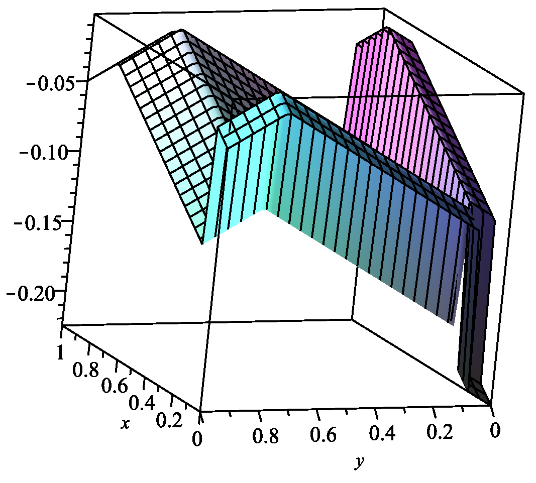
we get that the inequality F ( x ) F ( u ) = 0.1 β 1 0 + β 1 0.7 β 1 | x F ( x ) | + β 1 | u F ( u ) | will hold for any β 1 [ 1 / 7 , 1 / 2 ) (Figure 1).
Let y , v [ 0 , 0.1 ] or y , v ( 0.1 , 1 ] , then:
F 2 ( y ) F 2 ( v ) = 0 β 2 | y F 2 ( y ) | + β 2 | v F 2 ( v ) |
holds for any β 2 [ 0 , 1 / 2 ) .
Let y [ 0 , 0.1 ] and v ( 0.1 , 1 ] , then, using the equalities:
0.8 = inf { | y F 2 ( y ) | : x [ 0 , 0.1 ] } and 0 = inf { | v F 2 ( v ) | : u ( 0.1 , 1 ] } ,
we get that the inequality:
F 2 ( y ) F 2 ( v ) = 0.1 β 2 0.8 + β 2 0 β 2 | y F 2 ( y ) | + β 2 | v F 2 ( v ) |
will hold for any β 2 [ 1 / 8 , 1 / 2 ) (Figure 2).
Therefore,
S 6 = F 1 ( x ) F 1 ( u ) + F 2 ( y ) F 2 ( v ) 1 7 | x F 1 ( x ) | + | u F 1 ( u ) | + | y F 2 ( y ) | + | v F 2 ( v ) | ,
and thus, the ordered pair ( F 1 , F 2 ) satisfies Assumption 3 with a constant β = 1 / 7 . Consequently, there exists an equilibrium pair ( x , y ) , and, for any initial start in the economy, the iterated sequences ( x n , y n ) converge to the market equilibrium ( x , y ) . In this case we get that the equilibrium pair of the production of the two firms is ( 0.8 , 0.1 ) .
The considered model with response functions F 1 and F 2 does not satisfy (10). Indeed, let us consider x = 0.8 , u = x + ε , and y = 0.1 , v = y + ε . Then
F 1 ( x ) F 1 ( u ) + F 2 ( y ) F 2 ( v ) = 0.1 + 0.1 = 0.2 2 ε = 2 ( | x u | + | y v | )
for any ε 0.1 , and thus, we cannot apply Assumption 1.
The example shows that if the values for F i were obtained by solving the optimization of the payoff functions, then we could not speak about the second-order conditions, as F i would not be differentiable.

5. Discussion

We have presented a generalization of a fixed-point result [16], and we have illustrated some possible applications and consequences of the main result (Theorem 2). We have illustrated the connection between coupled fixed points and fixed points by considering a suitable product space. Thus, it is easy to see the natural generalizations of Kannan, Chatterjea, or Hardy–Roger types of maps. We illustrated a possible application in the investigation of market equilibrium for noncompetitive markets. We showed that the presented technique can be used to widen some known results [32]. Thus, Assumption 1 covers any cases that are not covered by the classical first- and second-order conditions used in [32]. The main result (Theorem 2) can be used in more-complicated models, where we have considered a real-life model of duopolies by paying attention to the surplus of the total production. We compared the equilibrium obtained in both models in cases where the surplus was either considered or disregarded. We presented an example where the payoff functions may be non-differentiable, and thus, the classical first- and second-order conditions cannot be applied.

Author Contributions

Formal analysis: S.K., V.Z. and B.Z.; Methodology: S.K., V.Z. and B.Z. The listed authors have contributed equally in the research and are listed in alphabetical order. All authors have read and agreed to the published version of the manuscript.

Funding

This research was partially supported by two projects: KP-06 K2-29 “Integrated model for prediction and prevention of negative social and economic effects from future epidemic crises”, funded by the Bulgarian National Science Fund (BNSF)—“Funding of fundamental research projects on public challenges associated with the COVID-19 pandemic—2020”; UIA05-202 “INNOAIR—Innovative demand responsive green public transportation for cleaner air in urban environment”, funded by the European Union initiative—Urban Innovative Actions (UIA).

Institutional Review Board Statement

Not applicable.

Informed Consent Statement

Not applicable.

Data Availability Statement

Not applicable.

Acknowledgments

The authors would like to thank the anonymous reviewers for their comments and recommendations that have improved the value of the article.

Conflicts of Interest

The authors declare no conflict of interest.

References

  1. Guo, D.; Lakshmikantham, V. Coupled fixed points of nonlinear operators with application. Nonlinear Anal. 1987, 11, 623–632. [Google Scholar] [CrossRef]
  2. Radenović, S. Coupled fixed point theorems for monotone mappings in partially ordered metric spaces. Kragujev. J. Math. 2014, 38, 249–257. [Google Scholar] [CrossRef]
  3. Dorić, D.; Kadelburg, Z.; Radenović, S. Coupled fixed point results for mappings without mixed monotone property. Appl. Math. Lett. 2012, 25, 1803–1808. [Google Scholar] [CrossRef] [Green Version]
  4. Tian, J.; Hu, X.; O’regan, D. On ψ–contractions and common fixed point results in probabilistic metric spaces. Fixed Point Theory 2020, 21, 319–338. [Google Scholar] [CrossRef]
  5. Sharma, Y.; Jain, S. Coupled Fixed Point Theorems in Modular Metric Spaces Endowed with a Graph. Kyungpook Math. J. 2021, 61, 441–453. [Google Scholar] [CrossRef]
  6. Boudaoui, A.; Mebarki, K.; Shatanawi, W.; Abodayeh, K. Solution of some impulsive differential equations via coupled fixed point. Symmetry 2021, 13, 501. [Google Scholar] [CrossRef]
  7. Waheed, M.; Rehman, S.; Jan, N.; Gumaei, A.; Al-Rakhami, M. Some New Coupled Fixed-Point Findings Depending on Another Function in Fuzzy Cone Metric Spaces with Application. Math. Probl. Eng. 2021, 2021, 4144966. [Google Scholar] [CrossRef]
  8. Karusala, K.; Namana, S.; Mishra, L. Coupled fixed points theorems for generalized weak contractions in ordered b-metric spaces. Asian-Eur. J. Math. 2021, 2021, 2250050. [Google Scholar] [CrossRef]
  9. Ghasab, E.; Majani, H. Function weighted g–metric spaces and hausdorff Δ–distances; an application to fixed point theory. Int. J. Nonlinear Anal. Appl. 2021, 12, 1441–1452. [Google Scholar] [CrossRef]
  10. Sintunavarat, W.; Kumam, P. Coupled best proximity point theorem in metric Spaces. Fixed Point Theory Appl. 2012, 2012, 93. [Google Scholar] [CrossRef] [Green Version]
  11. Konar, P.; Chandok, S.; Dutta, S.; De la Sen, M. Coupled optimal results with an application to nonlinear integral equations. Axioms 2021, 10, 73. [Google Scholar] [CrossRef]
  12. Khazou, M.; Taoudi, M. Existence and uniqueness of fixed points for monotone operators in partially ordered Banach spaces and applications. J. Fixed Point Theory Appl. 2021, 23, 12. [Google Scholar] [CrossRef]
  13. Fazli, H.; Nieto, J. Fractional Langevin equation with anti-periodic boundary conditions. Chaos Solitons Fractals 2018, 114, 332–337. [Google Scholar] [CrossRef]
  14. Nashine, H.; Ibrahim, R. Monotone solutions of iterative fractional equations found by modified Darbo-type fixed-point theorems. J. Fixed Point Theory Appl. 2017, 19, 3217–3229. [Google Scholar] [CrossRef]
  15. Ramadan, M.; El-Shazly, N. On the Maximal Positive Definite Solution of the Nonlinear Matrix Equation (Formula presented). Appl. Math. Inf. Sci. 2020, 14, 349–354. [Google Scholar] [CrossRef]
  16. Dzhabarova, Y.; Kabaivanov, S.; Ruseva, M.; Zlatanov, B. Existence, Uniqueness and Stability of Market Equilibrium in Oligopoly Markets. Adm. Sci. 2020, 10, 70. [Google Scholar] [CrossRef]
  17. Kabaivanov, S.; Zlatanov, B. A variational principle, coupled fixed points and market equilibrium. Nonlinear Anal. Model. Control. 2021, 26, 169–185. [Google Scholar] [CrossRef]
  18. Gecheva, G.; Hristov, M.; Nedelcheva, D.; Ruseva, M.; Zlatanov, B. Applications of coupled fixed points for multivalued maps in the equilibrium in duopoly markets and in aquatic ecosystems. Axioms 2021, 10, 44. [Google Scholar] [CrossRef]
  19. Choudhury, B.; Metiya, N.; Kundu, S. Existence, uniqueness and well-posedness results for relation theoretic coupled fixed points problem using C–class function with some consequences and an application. J. Anal. 2021, 29, 227–245. [Google Scholar] [CrossRef]
  20. Petruşel, A. Fixed points vs. coupled fixed points. J. Fixed Point Theory Appl. 2018, 20, 150. [Google Scholar] [CrossRef]
  21. Cournot, A.A. Researches into the Mathematical Principles of the Theory of Wealth; Macmillan: New York, NY, USA, 1897. [Google Scholar]
  22. Udhayanan, P.; Mishra, S.; Rao, S. Firm dynamics and employee performance management in duopoly markets. Phys. A Stat. Mech. Appl. 2021, 583, 126298. [Google Scholar] [CrossRef]
  23. Gutiérrez, O. Planned Obsolescence with Network Effects. Rev. Netw. Econ. 2021, 19, 221–247. [Google Scholar] [CrossRef]
  24. Okuguchi, K.; Szidarovszky, F. The Theory of Oligopoly with Multi–Product Firms; Springer: Berlin/Heidelberg, Germany, 1990. [Google Scholar]
  25. Bischi, G.; Chiarella, C.; Kopel, M.; Szidarovszky, F. Nonlinear Oligopolies Stability and Bifurcations; Springer: Berlin/Heidelberg, Germany, 2010. [Google Scholar]
  26. Matsumoto, A.; Szidarovszky, F. Dynamic Oligopolies with Time Delays; Springer Nature Singapore Pte Ltd.: Singapore, 2018. [Google Scholar]
  27. Reich, S. Kannan’s fixed point theorem. Bull. Univ. Mat. Ital. 1971, 4, 1–11. [Google Scholar]
  28. Hardy, G.; Rogers, T. A generalization of a fixed point theorem of Reich. Canad. Math. Bull. 1973, 16, 201–206. [Google Scholar] [CrossRef]
  29. Kannan, R. Some results on fixed points. Bull. Calcutta Math. Soc. 1968, 10, 71–76. [Google Scholar]
  30. Chatterjea, S. Fixed-point theorems. Bull. Calcutta Math. Soc. 1972, 25, 727–730. [Google Scholar] [CrossRef]
  31. Friedman, J.W. Oligopoly Theory; Cambradge University Press: Cambridge, UK, 1983; Online publication date: September 2009. [Google Scholar] [CrossRef]
  32. Andaluz, J.; Elsadany, A.A.; Jarne, G. Dynamic Cournot oligopoly game based on general isoelastic demand. Nonlinear Dyn. 2020, 99, 1053–1063. [Google Scholar] [CrossRef]
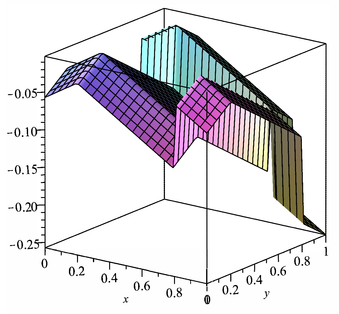
Figure 1. Graphic of the function | F ( x ) F ( y ) | 1 7 ( | x F ( x ) | + | y F ( y ) | ) .
Symmetry 14 00605 g001
Figure 2. Graphic of the function | F 2 ( y ) F 2 ( v ) | 1 8 ( | y F 2 ( y ) | + | v F 2 ( v ) | ) .
Symmetry 14 00605 g002
Table 1. The iterated sequence’s values ( x n , y n ) with initial conditions of ( 20 , 31 ) .
n0123456
x n 20292417600100
y n 3118356710100
Table 2. The iterated sequence’s values ( x n , y n ) with initial conditions of ( 20 , 30 ) .
n0122k2k + 1
x n 2030202030
y n 3020303020
Table 3. The iterated sequence’s values ( x n , y n ) with initial values of ( 10 , 30 ) .
n01234510215051120121599600
x n 103712351333.716.830.821.126.922.6425.4324.0724.05
y n 301833203121.428.624.125.826.426.0326.3426.1926.18
Publisher’s Note: MDPI stays neutral with regard to jurisdictional claims in published maps and institutional affiliations.