Sec-G Class of Distributions: Properties and Applications

Abstract

Although there are many continuous distributions in the literature, only a handful take advantage of the modeling power provided by trigonometric functions. To our knowledge, none of them are based on the so-called secant function, defined as the reciprocal of the cosine function. The secant function can go to large values whenever the cosine function goes to small values. The idea is to profit from this trigonometric property to modify well-known distribution tails and overall skewness features. With this in mind, in this paper, a new class of trigonometric distributions based on the secant function is introduced. It is called the Sec-G class. We discuss the main mathematical characteristics of this class, including series expansions of the corresponding cumulative distribution and probability density functions, as well as several probabilistic measures and functions. In particular, we present the moments, skewness, kurtosis, Lorenz, and Bonferroni curves, reliability coefficient, entropy measure, and order statistics. Throughout the study, emphasis is placed on the unique four-parameter continuous distribution of this class, defined with the Kumaraswamy-Weibull distribution as the baseline. The estimation of the model parameters is performed using the maximum likelihood method. We also carried out a numerical simulation study and present the results in graphic form. Three referenced datasets were analyzed, and it is proved that the proposed secant Kumaraswamy-Weibull model outperforms important competitors, including the Kumaraswamy-Weibull, Kumaraswamy-Weibull geometric, Kumaraswamy-Weibull Poisson, Kumaraswamy Burr XII, and Weibull models.

1. Introduction

Standard (continuous) distributions do not provide enough modeling flexibility to acceptably evaluate all types of data. It is especially true for data with unusual tails, skewness, or kurtosis characteristics. To bridge that gap, researchers have proposed many classes of distributions in recent literature, attempting to broaden the properties of existing distributions. The majority are created by changing basic baseline distributions. The most popular transformations are those that rely on analysis operators (power, integral, composition, …) and one or more tuning parameters. The unavoidable works in this regard are those of [1], introducing the exp-G class, Reference [2], presenting the Kumaraswamy-G class, Reference [3], introducing the Marshall–Olkin-G class, Reference [4], developing the beta-G class, and [5] introducing the gamma-G class. We also refer the reader to Table 1 of [6], which provides an exhaustive list of the most useful ones, with the references therein. Even with the advancements of modern applied science experiments, there is still a growing requirement for adaptable statistical models to adapt to all kinds of data, leading to the development of new approaches based on novel analytical techniques.

On the other hand, trigonometric functions have examples in different areas, such as mathematics, physics, biology, and engineering. The sine distribution was proposed by [7] in the last century. The model’s creation arose from the need to calculate the impact angles on the moon’s craters caused by the meteorite. In this context, Reference [8] proposed a system of distributions where the two cumulative distribution functions (CDFs) depend exclusively on tangent and sine functions, known as Burr type V and Burr type XI distributions. Although these distributions are not the most preferred by researchers, both distributions have numerous applications. Reference [9] proposed using the cosine distribution to approximate the normal distribution. The Beta trigonometric distribution, proposed by [10], can be used to model economic data. These famous circular distributions can be used in many applications, such as insect life, widely applied in geology [11]. In many phenomena, circular measurements, such as the movement direction of an animal after a given stimulus, wind direction analysis, the arrival time of a patient in a hospital, and insect visits in flowers, are also analyzed by these circular distributions.

As a result, logically, there is a growing interest in new distributions and classes of distributions based on trigonometric functions $sin\left(x\right)$, $cos\left(x\right)$, $tan\left(x\right)$, etc. Such classes take advantage of the curvature properties of these trigonometric functions to produce flexible distributions with desirable properties, in terms of modeling. In particular, greater power is gained in the tails without including new parameters. We can point the reader to the works of [12,13,14,15,16,17,18,19,20]. To the best of our knowledge, no class of distributions is centered on the secant function, defined as the reciprocal of the cosine function $sec\left(x\right)=1/cos\left(x\right)$. When the cosine function takes small values, the secant function takes large values. This characteristic could be useful for changing the tails and overall skewness of an existing distribution. With this in mind, in this research, we aimed to develop and analyze the secant generated (Sec-G) class of distributions, which are described by the following CDF:

$$\begin{array}{c}\hfill H(x;\zeta )=sec\left(\frac{\pi }{3}G(x;\zeta )\right)-1,x\in \mathbb{R},\end{array}$$

(1)

where $G(x;\zeta )$ is a CDF of a baseline (continuous) distribution depending on one or several parameters represented by $\zeta$. Further motivations behind the Sec-G class are the following ones:

(a)

Every chosen baseline distribution leads to a previously unstudied trigonometric distribution.

(b)

The corresponding CDF has a tractable expression, implying the same for all related functions (such as the probability density, hazard rate, and quantile functions), and there is no additional parameter to those of the baseline distribution.

(c)

One can prove that the following first-order stochastic dominance property: for any $x\in \mathbb{R}$, we have

$$H(x;\zeta )\le G(x;\zeta ).$$

It means that the Sec-G class stochastically dominates its baseline distribution; it provides a real alternative model compared to the baseline model in the CDF sense. For instance, the Sin-G class by [13,14] satisfies the exact reversed first-order stochastic dominance property, which makes the Sec-G class a complementary solution.

(d)

Thanks to the well-known series expansion function of the secant function, simple series expansions of some important functions are feasible.

(e)

More secondary, if we attempt to link the Sec-G class to the actual literature, we remark that it belongs to the general classes of distributions proposed by [21,22]. Indeed, we have $H(x;\zeta )={\int }_0^{G(x;\zeta )}r\left(t\right)dt$, where $r\left(t\right)=(\pi /3)sec(\pi t/3)tan(\pi t/3)$ defines a (new) generator probability density function (PDF).

(f)

The statistical models developed by the Sec-G class are manageable in terms of computing. They may be employed effectively in a real-data analysis situation.

All of those points are developed and discussed throughout the rest of the study. We emphasize the famous Kumaraswamy-Weibull (Kum-W) distribution introduced by [23] as the baseline, intending to create an alternative trigonometric four-parameter distribution with different levels of functionalities. This paper will show how the proposed distribution can outperform the goodness-of-fit power of the Kum-W distribution in a concrete data analysis scenario.

The paper is as follows: Section 2 provides the essential functions of the Sec-G class, with a focus on the Kum-W distribution as the baseline. The main properties of the class are discussed in Section 3. Applications to simulated and real-life data are given in Section 4. Some concluding remarks are formulated in Section 5.

2. Basics on the Sec-G Class

Here, we complete the presentation of the Sec-G class, with a focus on its main functions of interest.

2.1. Main Functions

First, we recall that the Sec-G class is defined by the CDF $H(x;\zeta )$, given by Equation (1). Clearly, by the definition of $H(x;\zeta )$, the support of the corresponding distribution corresponds to the support of the baseline distribution. In addition, it is worth noting that the Sec-G class is identifiable if and only if the baseline distribution is identifiable. That is, the equality $H(x;{\zeta }_1)=H(x;{\zeta }_2)$ is equivalent to $G(x;{\zeta }_1)=G(x;{\zeta }_2)$, which is equivalent to ${\zeta }_1={\zeta }_2$.

As another important function of the Sec-G class, the survival function, is given by $S(x;\zeta )=1-H(x;\zeta )$, that is

$$\begin{array}{c}\hfill S(x;\zeta )=2-sec\left(\frac{\pi }{3}G(x;\zeta )\right),x\in \mathbb{R}.\end{array}$$

Upon differentiation of $H(x;\zeta )$ with respect to x, the corresponding PDF is given by

$$\begin{array}{c}\hfill h(x;\zeta )=\frac{\pi }{3}g(x;\zeta )sec\left({\displaystyle \frac{\pi }{3}}G(x;\zeta )\right)tan\left({\displaystyle \frac{\pi }{3}}G(x;\zeta )\right),x\in \mathbb{R},\end{array}$$

(2)

where $g(x;\zeta )$ denotes the PDF corresponding to $G(x;\zeta )$.

Moreover, the cumulative hazard rate function of the Sec-G class can be expressed as $\mathsf{\Omega }(x;\zeta )=-log\left[S\right(x;\zeta \left)\right]$; that is

$$\mathsf{\Omega }(x;\zeta )=-log\left. [2-sec\left(\frac{\pi }{3}G(x;\zeta )\right)\right],x\in \mathbb{R}.$$

The corresponding hazard rate function (HRF) is obtained upon differentiation of $\mathsf{\Omega }(x;\zeta )$ with respect to x; that is

$$\begin{array}{c}\hfill R(x;\zeta )={\displaystyle \frac{{\displaystyle \frac{\pi }{3}}g(x;\zeta )sec\left({\displaystyle \frac{\pi }{3}}G(x;\zeta )\right)tan\left({\displaystyle \frac{\pi }{3}}G(x;\zeta )\right)}{2-sec\left({\displaystyle \frac{\pi }{3}}G(x;\zeta )\right)}},x\in \mathbb{R}.\end{array}$$

These functions are essential for analyzing all possibilities of the Sec-G class in a practical setting. In particular, functions $h(x;\zeta )$ and $R(x;\zeta )$ are very informative about the modeling properties of the related distributions; the more they show various forms of shapes, the more the flexibility of the related distribution is desirable from a statistical point of view.

Another important function is the quantile function, defined as the inverse function of $H(x;\zeta )$. After some algebra, we get

$$\begin{array}{c}\hfill Q(u;\zeta )=Q_{*}\left({\displaystyle \frac{3}{\pi }}arcsec(u+1);\zeta \right),u\in (0,1),\end{array}$$

where $Q_{*}(u;\zeta )$ denotes the quantile function corresponding to $G(x;\zeta )$ and $arcsec\left(x\right)$ denotes the arcsecant function, defined as the inverse function of $sec\left(x\right)$, i.e., $arcsec\left(x\right)=arcos(1/x)$. To our knowledge, the Sec-G class is the first one with a quantile function depending on the arcsecant function. Then, we can express the three quartiles, including the median, as $M=Q(0.5;\zeta )$. We can also define some measures of skewness and kurtosis, such as the MacGillivray skewness proposed by [24] and the Moors kurtosis introduced by [25]. Finally, by considering a random variable U following the uniform distribution over $(0,1)$, we can generate values from the Sec-G class from generated values from U, by using the fact that $Q(U;\zeta )$ has the CDF of the Sec-G class as defined by Equation (1).

2.2. On the Shapes of the PDF and HRF

Here, we derive the basics on the shapes of the PDF and HRF of the Sec-G class. First, the derivative of $log\left[h\right(x;\zeta \left)\right]$ with respect to x is

$$\begin{array}{cc}\hfill {\left\{log\left[h\right(x;\zeta \left)\right]\right\}}^{\prime }& =\frac{g{(x;\zeta )}^{\prime }}{g(x;\zeta )}+\frac{\pi }{3}g(x;\zeta )tan\left({\displaystyle \frac{\pi }{3}}G(x;\zeta )\right)+\frac{\pi }{3}g(x;\zeta )\frac{{\left. [sec\left({\displaystyle \frac{\pi }{3}}G(x;\zeta )\right)\right]}^2}{tan\left({\displaystyle \frac{\pi }{3}}G(x;\zeta )\right)}.\hfill \end{array}$$

Thus, the critical point(s) of $h(x;\zeta )$ is (are) the root(s) of the following non-linear equation: ${\left\{log\left[h\right(x;\zeta \left)\right]\right\}}^{\prime }=0$. Such a critical point, say $x_o$, corresponds to a local maximum, a local minimum, or a point of inflection, depending on whether $\kappa <0$, $\kappa >0$ or $\kappa =0$, where $\kappa ={\left\{log\left[h\right(x;\zeta \left)\right]\right\}}^{″}{\mid }_{x=x_o}$.

The same methodology holds for the HRF of the Sec-G class. Indeed, the derivative of $log\left[R\right(x;\zeta \left)\right]$ with respect to x is

$$\begin{array}{cc}\hfill {\left\{log\left[R\right(x;\zeta \left)\right]\right\}}^{\prime }& =\frac{g{(x;\zeta )}^{\prime }}{g(x;\zeta )}+\frac{\pi }{3}g(x;\zeta )\frac{{\left. [sec\left({\displaystyle \frac{\pi }{3}}G(x;\zeta )\right)\right]}^2}{tan\left({\displaystyle \frac{\pi }{3}}G(x;\zeta )\right)}+{\displaystyle \frac{2\pi }{3}}g(x;\zeta ){\displaystyle \frac{tan\left({\displaystyle \frac{\pi }{3}}G(x;\zeta )\right)}{2-sec\left({\displaystyle \frac{\pi }{3}}G(x;\zeta )\right)}}.\hfill \end{array}$$

Thus, the critical point(s) of $R(x;\zeta )$ is(are) the root(s) of the following non-linear equation: ${\left\{log\left[R\right(x;\zeta \left)\right]\right\}}^{\prime }=0$. Again, such a critical point, say $x_{*}$, corresponds to a local maximum, a local minimum or a point of inflection, depending on whether $\upsilon <0$, $\upsilon >0$ or $\upsilon =0$, where $\upsilon ={\left\{log\left[R\right(x;\zeta \left)\right]\right\}}^{″}{\mid }_{x=x_{*}}$.

Let us now derive some asymptotic results on these functions. First, we recall that: when $y\to 0$, $sec\left((\pi /3)y\right)-1\sim ({\pi }^2/18)y^2$ and $tan\left(\right(\pi /3\left)y\right)\sim (\pi /3)y$, and, when $y\to 1$, $sec\left((\pi /3)y\right)-1\sim 1-(2\pi /\sqrt{3})(1-y)$ and $tan\left((\pi /3)y\right)\sim \sqrt{3}-(4\pi /3)(1-y)$. Therefore, when $G(x;\zeta )\to 0$, we have the following equivalences:

$$H(x;\zeta )\sim \frac{{\pi }^2}{18}G{(x;\zeta )}^2,h(x;\zeta )\sim \frac{{\pi }^2}{9}g(x;\zeta )G(x;\zeta ),R(x;\zeta )\sim \frac{{\pi }^2}{9}g(x;\zeta )G(x;\zeta ).$$

Moreover, when $G(x;\zeta )\to 1$, we have the following equivalences:

$$H(x;\zeta )\sim 1-\frac{2\pi }{\sqrt{3}}(1-G(x;\zeta )),h(x;\zeta )\sim \frac{2\pi }{\sqrt{3}}g(x;\zeta ),R(x;\zeta )\sim \frac{g(x;\zeta )}{1-G(x;\zeta )}.$$

For a given baseline CDF $G(x;\zeta )$, these results are helpful in determining the asymptotic comportments of the PDF and HRF of the corresponding distribution. This point is illustrated in the next subsection by considering a special member of the Sec-G class.

2.3. The Sec-Kum-W Distribution

The Sec-G class, due to its original definition, contains many new trigonometric distributions. Here, a promising one is presented. The Kum-W distribution defined it as the baseline. As a brief description, the Kum-W distribution was introduced by [23] with the CDF given by

$$G(x;\zeta )=1-{\left\{1-{\left. [1-exp(-{\left(\lambda x\right)}^c)\right]}^a\right\}}^b,x>0,$$

where $\zeta =(a,b,c,\lambda )$, $\lambda >0$ is a scale parameter, and $a,b,c>0$ are shape parameters, and the PDF is given by

$$g(x;\zeta )=abc{\lambda }^c{x}^{c-1}exp(-{\left(\lambda x\right)}^c){\left. [1-exp(-{\left(\lambda x\right)}^c)\right]}^{a-1}{\left\{1-{\left. [1-exp(-{\left(\lambda x\right)}^c)\right]}^a\right\}}^{b-1}.$$

The Kum-W distribution contains many well-referenced distributions. The most notable ones are the Weibull, exponentiated Weibull, and exponentiated exponential distributions (see [26]). Other examples are provided in Table 1 of [23]. The Kum-W distribution supports all five major HRF shapes: constant, increasing, decreasing, bathtub, and unimodal. In the last decade, the Kum-W distribution proved to be one of the more efficient lifetime distributions for data analysis. For further information, see, for instance [27,28,29].

Thus, in this part, we propose an extension of the Kum-W distribution that first-order stochastically dominates it, with a similar level of flexibility. We define the Sec-Kum-W distribution by the CDF given by Equation (1) with $G(x;\zeta )$ as the CDF of the Kumaraswamy-Weibull distribution; that is

$$\begin{array}{c}\hfill H(x;\zeta )=sec\left(\frac{\pi }{3}\left(1-{\left\{1-{\left. [1-exp(-{\left(\lambda x\right)}^c)\right]}^a\right\}}^b\right)\right)-1,x>0.\end{array}$$

(3)

It thus satisfies the following first-order stochastic dominance property: $H(x;\zeta )\le G(x;\zeta )$ for any $x\in \mathbb{R}$. Then, all of the functions presented in the previous section can be expressed. In particular, the corresponding PDF and HRF are, respectively, obtained as

$$\begin{array}{cc}\hfill h(x;\zeta )& =\frac{\pi }{3}abc{\lambda }^c{x}^{c-1}exp(-{\left(\lambda x\right)}^c){\left. [1-exp(-{\left(\lambda x\right)}^c)\right]}^{a-1}{\left\{1-{\left. [1-exp(-{\left(\lambda x\right)}^c)\right]}^a\right\}}^{b-1}\hfill \\ \hfill & \times sec\left(\frac{\pi }{3}\left(1-{\left\{1-{\left. [1-exp(-{\left(\lambda x\right)}^c)\right]}^a\right\}}^b\right)\right)tan\left(\frac{\pi }{3}\left(1-{\left\{1-{\left. [1-exp(-{\left(\lambda x\right)}^c)\right]}^a\right\}}^b\right)\right),\hfill \\ \hfill x>0\end{array}$$

(4)

and

$$\begin{array}{cc}\hfill R(x;\zeta )& =\frac{\pi }{3}abc{\lambda }^c{x}^{c-1}exp(-{\left(\lambda x\right)}^c){\left. [1-exp(-{\left(\lambda x\right)}^c)\right]}^{a-1}{\left\{1-{\left. [1-exp(-{\left(\lambda x\right)}^c)\right]}^a\right\}}^{b-1}\hfill \\ \hfill & \times \frac{sec\left({\displaystyle \frac{\pi }{3}}\left(1-{\left\{1-{\left. [1-exp(-{\left(\lambda x\right)}^c)\right]}^a\right\}}^b\right)\right)tan\left({\displaystyle \frac{\pi }{3}}\left(1-{\left\{1-{\left. [1-exp(-{\left(\lambda x\right)}^c)\right]}^a\right\}}^b\right)\right)}{2-sec\left({\displaystyle \frac{\pi }{3}}\left(1-{\left\{1-{\left. [1-exp(-{\left(\lambda x\right)}^c)\right]}^a\right\}}^b\right)\right)},\hfill \\ \hfill x>0.\end{array}$$

Moreover, the quantile function of the Sec-Kum-W distribution is specified by

$$\begin{array}{c}\hfill Q(u;\zeta )=\frac{1}{\lambda }{\left. [-log\left\{1-{\left. [1-{\left(1-{\displaystyle \frac{3}{\pi }}arcsec(u+1)\right)}^{1/b}\right]}^{1/a}\right\}\right]}^{1/c},u\in (0,1).\end{array}$$

In particular, this analytical expression allows us the simulation of random values from the Sec-Kum-W distribution.

The critical points and asymptotic properties of $h(x;\zeta )$ and $R(x;\zeta )$ can be determined by using the non-linear equations presented in the above section. Due to their analytical complexity, a mathematical software can help to obtain precise calculations of the critical points. On the other hand, by using Section 3 of [23], we arrive at the following equivalences. When $x\to 0$, we get

$$H(x;\zeta )\sim \frac{{\pi }^2}{18}{b}^2{\lambda }^{2ac}{x}^{2ac},h(x;\zeta )\sim \frac{{\pi }^2}{9}a{b}^{2}c{\lambda }^{2ac}{x}^{2ac-1},R(x;\zeta )\sim \frac{{\pi }^2}{9}a{b}^{2}c{\lambda }^{2ac}{x}^{2ac-1}.$$

Moreover, when $x\to +\infty$, we have the following equivalences:

$$H(x;\zeta )\sim 1-\frac{2\pi }{\sqrt{3}}{a}^{b}exp(-b{\left(\lambda x\right)}^c),h(x;\zeta )\sim \frac{2\pi }{\sqrt{3}}{a}^{b}bc{\lambda }^c{x}^{c-1}exp(-b{\left(\lambda x\right)}^c),R(x;\zeta )\sim bc{\lambda }^c{x}^{c-1}.$$

As a consequence, when $x\to 0$, $h(x;\zeta )\to 0$ for $2ac>1$, $h(x;\zeta )\to ({\pi }^2/18)b^2\lambda$ for $2ac=1$, and $h(x;\zeta )\to +\infty$ for $2ac<1$. The same asymptotes hold for $R(x;\zeta )$. Moreover, when $x\to +\infty$, $h(x;\zeta )\to 0$ in all circumstances, whereas $R(x;\zeta )\to 0$ for $c<1$, $R(x;\zeta )\to b\lambda$ for $c=1$, and $R(x;\zeta )\to +\infty$ for $c>1$. One can remark that, as for the former Kumaraswamy-Weibull distribution, the (asymptotic) tails of $h(x;\zeta )$ are of different nature: the upper tail is of exponential type whereas the lower tail is of polynomial type.

The main interest of the Sec-Kum-W distribution is to possess very flexible PDF and HRF. This aspect is difficult to reveal from an analytical approach, which motivates us to provide graphic evidence. Thus, Figure 1 and Figure 2 present some curves of these two functions for selected values of the parameters, respectively.

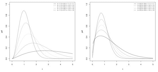
Figure 1. Plots of the PDF of the Sec-Kum-W distribution for some selected values of the parameters.

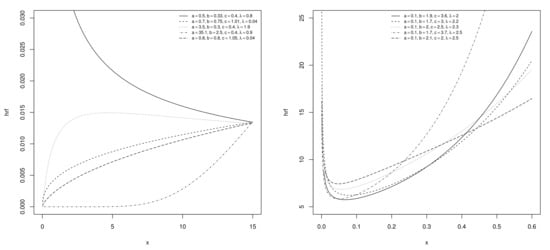
Figure 2. Plots of the HRF of the Sec-Kum-W distribution for some selected values of the parameters.

We see in Figure 1 that the PDF of the Sec-Kum-W distribution presents great flexibility in the central and dispersion parameters (mean, modes, variance…), skewness, and kurtosis, observing highly-right skewed as well as near-symmetrical curves. Comparatively, the Sec-Kum-W distribution’s PDF is more flexible in the right tail and kurtosis level than the PDF of the Kum-W distribution. However, it appears less likely to modulate the left tail (see Figure 1 of [23]).

From Figure 2, we see that the corresponding HRF can have constant, increasing, decreasing, bathtub, and unimodal shapes. Moreover, different levels of convexity–concavity are observed. From the statistical modeling point of view, these are very desirable properties. Comparatively, we can observe that the HRF of the Sec-Kum-W distribution can be increasing and concave (for $(a,b,c,\lambda )=(3.5,0.3,0.4,1.9)$, for instance), which is less immediate for the HRF of the Kum-W distribution (see Figure 2 of [23]).

3. Mathematical Properties

Here, the main mathematical properties of the Sec-G class are derived, with applications to the Sec-Kum-W distribution when appropriate.

3.1. Useful Series Expansions

The following result presents useful series expansions for the CDF and PDF of the Sec-G class in terms of CDFs and PDFs of the exp-G class introduced by [1].

Theorem 1.

The CDF and PDF of the Sec-G class given by Equations (1) and (2) can be expressed as

$$\begin{array}{c}\hfill H(x;\zeta )=\sum _{k=1}^{+\infty }{\omega }_k{G}_{2k}(x;\zeta ),h(x;\zeta )=\sum _{k=1}^{+\infty }{\omega }_k{g}_{2k}(x;\zeta ),\end{array}$$

respectively, where

$${\omega }_k={\left({\displaystyle \frac{\pi }{3}}\right)}^{2k}{\displaystyle \frac{{(-1)}^k{E}_{2k}}{\left(2k\right)!}},$$

$E_{2k}$is the Euler number, $G_{2k}(x;\zeta )=G{(x;\zeta )}^{2k}$ and $g_{2k}(x;\zeta )=2kg(x;\zeta )G{(x;\zeta )}^{2k-1}$, which are the CDF and PDF of the exp-G class with a power parameter of $2k$, respectively.

Proof. 

The proof is centered around the following well-established result. For any $y\in (-\pi /2,\pi /2)$, the secant function has the following series expansion:

$$sec\left(y\right)=\sum _{k=0}^{+\infty }{\displaystyle \frac{{(-1)}^k{E}_{2k}}{\left(2k\right)!}}{y}^{2k}.$$

We may refer the reader to [30], and the references therein. Therefore, since $(\pi /3)G(x;\zeta )$$\in (0,\pi /3)$, we can express the CDF of the Sec-G class as

$$\begin{array}{c}\hfill H(x;\zeta )=\sum _{k=1}^{+\infty }{\displaystyle \frac{{(-1)}^k{E}_{2k}}{\left(2k\right)!}}{\left({\displaystyle \frac{\pi }{3}}G(x;\zeta )\right)}^{2k}=\sum _{k=1}^{+\infty }{\omega }_{k}G{(x;\zeta )}^{2k}.\end{array}$$

(5)

Upon differentiation of the above function with respect to x, the desired series expansion for $h(x;\zeta )$ follows. This ends the proof of Theorem 1. □

As an example, let us consider the Sec-Kum-W distribution, defined by the CDF and PDF given by Equations (3) and (4), respectively. Then, the CDF of the Sec-Kum-W distribution can be expressed as

$$\begin{array}{c}\hfill H(x;\zeta )=\sum _{k=1}^{+\infty }{\omega }_k{G}_{2k}(x;\zeta ),\end{array}$$

with, by applying the (standard and generalized) binomial formula three times in a row,

$$\begin{array}{cc}\hfill G_{2k}(x;\zeta )& ={\left. [1-{\left\{1-{\left. [1-exp(-{\left(\lambda x\right)}^c)\right]}^a\right\}}^b\right]}^{2k}\hfill \\ \hfill & =\sum _{j=0}^{2k}\sum _{l=0}^{+\infty }\sum _{s=0}^{+\infty }\left(\genfrac{}{}{0pt}{}{2k}{j}\right)\left(\genfrac{}{}{0pt}{}{bj}{l}\right)\left(\genfrac{}{}{0pt}{}{al}{s}\right){(-1)}^{j+l+s}exp(-s{\left(\lambda x\right)}^c).\hfill \end{array}$$

Moreover, the corresponding PDF can be expressed as

$$\begin{array}{c}\hfill h(x;\zeta )=\sum _{k=1}^{+\infty }{\omega }_k{g}_{2k}(x;\zeta ),\end{array}$$

(6)

where

$$\begin{array}{c}\hfill g_{2k}(x;\zeta )=\sum _{j=0}^{2k}\sum _{l=0}^{+\infty }\sum _{s=1}^{+\infty }\left(\genfrac{}{}{0pt}{}{2k}{j}\right)\left(\genfrac{}{}{0pt}{}{bj}{l}\right)\left(\genfrac{}{}{0pt}{}{al}{s}\right){(-1)}^{j+l+s+1}{q}_s(x;\zeta ),\end{array}$$

(7)

and $q_s(x;\zeta )=cs{\lambda }^c{x}^{c-1}exp(-s{\left(\lambda x\right)}^c)$, corresponding to the PDF of the Weibull distribution with scale parameter of $s^{1/c}\lambda$ and shape parameter of c.

We can notice that $G_{2k}(x;\zeta )$ and $g_{2k}(x;\zeta )$ correspond to the CDF and PDF of the exponentiated Kumaraswamy-Weibull distribution with a power parameter of $2k$, respectively, which was studied in [27]. Thus, some results in [27] can be transposed in the context of the Sec-Kum-W distribution.

3.2. Moments

We now investigate some exploitable expressions for various moments or derivations. Let X be a random variable having the CDF and PDF of the Sec-G class given by Equations (1) and (2), respectively. Then, for any function $\psi \left(x\right)$ providing that the coming integral term exists, we have

$$\begin{array}{c}\hfill {\mathsf{{\rm Y}}}_{\psi }\left(X\right)=E\left[\psi \left(X\right)\right]={\int }_{-\infty }^{+\infty }\psi \left(x\right)h(x;\zeta )dx.\end{array}$$

In most cases, the integral term can be calculated numerically by the use of a mathematical software. A tractable series expansion is also available based on Theorem 1; we have

$$\begin{array}{c}\hfill {\mathsf{{\rm Y}}}_{\psi }\left(X\right)=\sum _{k=1}^{+\infty }{\omega }_k{\int }_{-\infty }^{+\infty }\psi \left(x\right)g_{2k}(x;\zeta )dx.\end{array}$$

(8)

According to the complexity of $g_{2k}(x;\zeta )$, the integral term can have an analytical expression. Thus, for a large integer K, the following finite sum can provide a suitable approximation for ${\mathsf{{\rm Y}}}_{\psi }\left(X\right)$:

$$\begin{array}{c}\hfill {\mathsf{{\rm Y}}}_{\psi }\left(X\right)\approx \sum _{k=1}^K{\omega }_k{\int }_{-\infty }^{+\infty }\psi \left(x\right)g_{2k}(x;\zeta )dx.\end{array}$$

Table 1 lists several well-known measures or functions related to the concept of moments based on specific choices for $\psi \left(x\right)$, including the mean, raw moments, variance, central moments, moment generating function, characteristic functions, and incomplete moments.

Table 1. Well-known measures or functions related to the concept of moments.

${{{\rm Y}}}_{\mathit{\psi }}\left(\mathit{X}\right)$	$\mathit{\psi }\left(\mathit{x}\right)$	Notation
mean	x	$\mu$
$m^{th}$ raw moment	$x^m$	${\mu }_m^{\prime }$
variance	${(x-\mu )}^2$	${\sigma }^2$
$m^{th}$ central moment	${\displaystyle {(x-\mu )}^m=\sum _{q=0}^m\left(\genfrac{}{}{0pt}{}{m}{q}\right){(-1)}^q{\mu }^q{x}^{m-q}}$	${\mu }_m$
$m^{th}$ descending factorial moment	$x(x-1)(x-2)\dots (x-m+1)$	${\mu }_{\left(m\right)}^{\prime }$
moment generating function in t	$e^{tx}$	$M\left(t\right)$
characteristic function in t	$e^{itx}$	$\phi \left(t\right)$
$m^{th}$ incomplete moment in t	$x^m$ if $x\le t$, 0 if $x>t$	${\mu }_m\left(t\right)$

The result below illustrates the interest of Equation (8) by determining a tractable series expansion for the $m^{th}$ raw moment of a random variable following the Sec-Kum-W distribution.

Proposition 1.

Let X be a random following the Sec-Kum-W distribution, i.e., with CDF and PDF given by Equations (3) and (4), respectively. Then, the $m^{th}$ raw moment of X is given by

$$\begin{array}{c}\hfill {\mu }_m^{\prime }={\lambda }^{-m}\mathsf{\Gamma }\left(\frac{m}{c}+1\right)\sum _{k=1}^{+\infty }\sum _{j=0}^{2k}\sum _{l=0}^{+\infty }\sum _{s=1}^{+\infty }{\omega }_k\left(\genfrac{}{}{0pt}{}{2k}{j}\right)\left(\genfrac{}{}{0pt}{}{bj}{l}\right)\left(\genfrac{}{}{0pt}{}{al}{s}\right){(-1)}^{j+l+s+1}{s}^{-m/c},\end{array}$$

where $\mathsf{\Gamma }\left(x\right)={\int }_0^{+\infty }{t}^{x-1}{e}^{-t}dt$ is the so-called gamma function.

Proof. 

Owing to Equations (8) with $\psi \left(x\right)=x^m$, (7) and (6), we have

$$\begin{array}{cc}\hfill {\mu }_m^{\prime }& =E\left(X^m\right)=\sum _{k=1}^{+\infty }{\omega }_k{\int }_{-\infty }^{+\infty }{x}^m{g}_{2k}(x;\zeta )dx\hfill \\ \hfill & =\sum _{k=1}^{+\infty }\sum _{j=0}^{2k}\sum _{l=0}^{+\infty }\sum _{s=1}^{+\infty }{\omega }_k\left(\genfrac{}{}{0pt}{}{2k}{j}\right)\left(\genfrac{}{}{0pt}{}{bj}{l}\right)\left(\genfrac{}{}{0pt}{}{al}{s}\right){(-1)}^{j+l+s+1}{\int }_0^{+\infty }{x}^m{q}_s(x;\zeta )dx.\hfill \end{array}$$

Now, by applying the change of variable $y=s{\left(\lambda x\right)}^c$, we get

$$\begin{array}{c}\hfill {\int }_0^{+\infty }{x}^m{q}_s(x;\zeta )dx=cs{\lambda }^c{\int }_0^{+\infty }{x}^{m+c-1}exp(-s{\left(\lambda x\right)}^c)dx={\lambda }^{-m}{s}^{-m/c}\mathsf{\Gamma }\left(\frac{m}{c}+1\right).\end{array}$$

This ends the proof of Proposition 1.    □

With a slight modification, the $m^{th}$ incomplete moment of a random variable following the Sec-Kum-W distribution is given in the next result.

Proposition 2.

Let X be a random following the Sec-Kum-W distribution, i.e., with CDF and PDF given by Equations (3) and (4), respectively. Then, the $m^{th}$ incomplete moment of X with respect to t is given by

$$\begin{array}{c}\hfill {\mu }_m\left(t\right)={\lambda }^{-m}\sum _{k=1}^{+\infty }\sum _{j=0}^{2k}\sum _{l=0}^{+\infty }\sum _{s=1}^{+\infty }{\omega }_k\left(\genfrac{}{}{0pt}{}{2k}{j}\right)\left(\genfrac{}{}{0pt}{}{bj}{l}\right)\left(\genfrac{}{}{0pt}{}{al}{s}\right){(-1)}^{j+l+s+1}{s}^{-m/c}{\mathsf{\Gamma }}_L\left(\frac{m}{c}+1,s{\left(\lambda t\right)}^c\right),\end{array}$$

where ${\mathsf{\Gamma }}_L(x,y)={\int }_0^y{t}^{x-1}{e}^{-t}dt$ is the lower incomplete gamma function.

The proof of Proposition 2 follows the one of Proposition 1. It is thus omitted.

For measuring and visualizing income inequalities, the Bonferroni and Lorenz curves are commonly used. The Lorenz curve, denoted by $L\left(p\right)$, is the proportion of total income volume accumulated by those units with an income less than or equal to a certain volume, and the Bonferroni curve, denoted by $B\left(p\right)$, is the scaled conditional mean curve; that is, the population’s ratio of group mean income. In the setting of the Sec-G class, $L\left(p\right)$ and $B\left(p\right)$ are defined by

$$L\left(p\right)=\frac{{\mu }_1\left[Q(p;\zeta )\right]}{\mu },B\left(p\right)=\frac{{\mu }_1\left[Q(p;\zeta )\right]}{p\mu },p\in (0,1),$$

respectively. The plots of these two kinds of curve in the case of the Sec-Kum-W distribution are given in Figure 3 for $b=1$, $c=1$, and $\lambda =0.5$, and selected values for a.

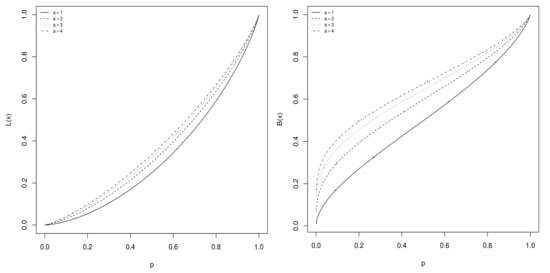
Figure 3. Plots of $L\left(p\right)$ and $B\left(p\right)$ for the Sec-Kum-W distribution for $b=1$, $c=1$, and $\lambda =0.5$, and selected values for a, and varying p.

We see that, for the considered values of the parameters, $L\left(p\right)$ is increasing and convex, whereas $B\left(p\right)$ is increasing with a tilde shape (concave, then convex, then concave).

For the special Sec-Kum-W distribution, the moment measures $\mu$ and ${\mu }_1\left(t\right)$ can be derived from Proposition 1 and Proposition 2, respectively.

We can express the central moments, moment generating function, and characteristic function in a similar manner. In addition, from the central moments and variance of X, we can define the $m^{th}$ general coefficient of the Sec-G class as

$$\begin{array}{c}\hfill C\left(m\right)={\displaystyle \frac{{\mu }_m}{{\sigma }^{m/2}}}.\end{array}$$

Then, $C\left(3\right)$ and $C\left(4\right)$ are used to calculate skewness and kurtosis. Thus, depending on $C\left(3\right)<0$, $C\left(3\right)=0$, or $C\left(3\right)>0$, the sign of $C\left(3\right)$ informs on the distribution’s left, symmetric, or right skewed nature, whereas the value of $C\left(4\right)$ informs on its tailedness. In order to see the numerical capabilities of these measures, some graphics are provided. For some parameter values of b, c, and $\lambda$, the skewness and kurtosis coefficients for the Sec-Kum-W distribution are plotted as functions of a in Figure 4, and as functions of b in Figure 5. In addition, for some parameter values of a, b, and $\lambda$, they are plotted as functions of c in Figure 6.

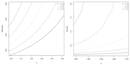
Figure 4. Plots of skewness and kurtosis coefficients of the Sec-Kum-W distribution as functions of a for $b=1.5$, $\lambda =2.5$, and selected values of c.

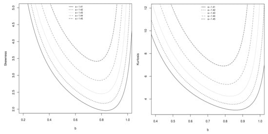
Figure 5. Plots of skewness and kurtosis coefficients of the Sec-Kum-W distribution as functions of b for $c=1.47$, $\lambda =2.4$, and selected values of a.

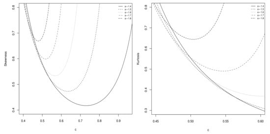
Figure 6. Plots of skewness and kurtosis coefficients of the Sec-Kum-W distribution as functions of c, for $b=1.50$, $\lambda =2.5$, and selected values of a.

From Figure 5 and Figure 6, we can see that the Sec-Kum-W is mainly a right skewed lifetime distribution. For a distribution of this kind, we observe the enormous flexibility that this new distribution presents in its asymmetry and kurtosis curves.

3.3. Coefficient of Reliability

We are now studying the coefficient of reliability of the Sec-G class via the concept described in [31]. Mathematically, it is expressed as

$$\begin{array}{c}\hfill R={\int }_{\mathbb{R}}{h}_1\left(x\right)H_2\left(x\right)dx,\end{array}$$

where $h_1\left(x\right)$ denotes the PDF of the Sec-G class as in Equation (2) with a baseline CDF given by $G(x;{\zeta }_1)$, and $H_2\left(x\right)$ denotes the CDF of the Sec-G class as in Equation (1) with a baseline CDF given by $G(x;{\zeta }_2)$. Hence, it is assumed that ${\zeta }_1$ and ${\zeta }_2$ are two parameter vectors, possibly different. The integral expression of R can be complicated to determine due to the complexity of the involved functions. However, a series expansion is possible thanks to the expansion of $h_1\left(x\right)$ and $H_2\left(x\right)$. From Equations (5) and (6), as well as the interchanged integral and sum signs, it follows that

$$\begin{array}{cc}\hfill R& ={\int }_{\mathbb{R}}\left. [\sum _{k=1}^{+\infty }{\omega }_k{g}_{2k}(x;{\zeta }_1)\right]\times \left. [\sum _{\ell =1}^{+\infty }{\omega }_{\ell }{G}_{2\ell }(x;{\zeta }_2)\right]dx=\sum _{k=1}^{+\infty }\sum _{\ell =1}^{+\infty }{\omega }_k{\omega }_{\ell }{\int }_{\mathbb{R}}{g}_{2k}(x;{\zeta }_1)G_{2\ell }(x;{\zeta }_2)dx.\hfill \end{array}$$

In an expanded form, we obtain

$$\begin{array}{cc}\hfill R& =2\sum _{k=1}^{+\infty }\sum _{\ell =1}^{+\infty }{\omega }_k{\omega }_{\ell }k{\int }_{\mathbb{R}}g(x;{\zeta }_1)G{(x;{\zeta }_1)}^{2k-1}G{(x;{\zeta }_2)}^{2\ell }dx.\hfill \end{array}$$

For given $G(x;{\zeta }_1)$ and $G(x;{\zeta }_2)$, this integral can be computed numerically.

As a consequence, if one can assume the existence of $\upsilon >0$ such that $G(x;{\zeta }_2)=G{(x;{\zeta }_1)}^{\upsilon }$, then we have the following simple series expansion:

$$\begin{array}{c}\hfill R=\sum _{k=1}^{+\infty }\sum _{\ell =1}^{+\infty }{\omega }_k{\omega }_{\ell }\frac{k}{k+\ell \upsilon }\end{array}$$

For $\upsilon =1$, we get the expected $R=1/2$.

3.4. Entropy Measure

The entropy of a distribution can be presented as a measure of uncertainty; the higher the entropy, the higher the disorder and the lower the chance of seeing a specific event. This part focuses on the Rényi entropy of the Sec-G class, as defined in a general way in [32]. Let $\gamma >0$ and $\gamma \ne 1$. Then, the Rényi entropy of the Sec-G class is specified by

$$\begin{array}{cc}\hfill \mathfrak{I}\left(\gamma \right)& =\frac{1}{1-\gamma }log\left. [{\int }_{\mathbb{R}}h{(x;\zeta )}^{\gamma }dx\right]={\displaystyle \frac{1}{1-\gamma }}log\left. [{\int }_{\mathbb{R}}{\left(\frac{\pi }{3}\right)}^{\gamma }g{(x;\zeta )}^{\gamma }sec{\left({\displaystyle \frac{\pi }{3}}G(x;\zeta )\right)}^{\gamma }tan{\left({\displaystyle \frac{\pi }{3}}G(x;\zeta )\right)}^{\gamma }dx\right].\hfill \end{array}$$

The calculus of $\mathfrak{I}\left(\gamma \right)$ is still possible with mathematical software. We propose here a series expansion approach. By virtue of the Taylor series of the function $sec{\left((\pi /3)u\right)}^{\gamma }tan{\left((\pi /3)u\right)}^{\gamma }$ at a given point $u=u_0$, we can write

$$\begin{array}{c}\hfill sec{\left({\displaystyle \frac{\pi }{3}}u\right)}^{\gamma }tan{\left({\displaystyle \frac{\pi }{3}}u\right)}^{\gamma }=\sum _{k=0}^{+\infty }\sum _{r=0}^k{a}_k\left(\genfrac{}{}{0pt}{}{k}{r}\right){(-1)}^{k-r}{u}_0^{k-r}{u}^r,\end{array}$$

where $a_k={\left. [sec{\left((\pi /3)u\right)}^{\gamma }tan{\left((\pi /3)u\right)}^{\gamma }\right]}^{\left(k\right)}{\mid }_{u=u_0}/k!$.

We get the following result after some algebra and the swapping of the integral and sum signs:

$$\begin{array}{c}\hfill \mathfrak{I}\left(\gamma \right)=\frac{1}{1-\gamma }\left\{\gamma log\left(\frac{\pi }{3}\right)+log\left. [\sum _{k=0}^{+\infty }\sum _{r=0}^k{a}_k\left(\genfrac{}{}{0pt}{}{k}{r}\right){(-1)}^{k-r}{u}_0^{k-r}{\int }_{\mathbb{R}}g{(x;\zeta )}^{\gamma }G{(x;\zeta )}^{r}dx\right]\right\}.\end{array}$$

In the vast majority of cases, $\mathfrak{I}\left(\gamma \right)$ can be computed numerically. This can be done for the Sec-Kum-W distribution, for instance. As a side note, the famous Shannon entropy is given by $\mathfrak{S}=-{\int }_{\mathbb{R}}log\left[h(x;\zeta )\right]h(x;\zeta )dx$. It corresponds to the limit case of $\mathfrak{I}\left(\gamma \right)$ when $\gamma$ tends to 1. Figure 7 presents some plots of the Rényi entropy for the Sec-Kum-W distribution with selected parameter values and varying $\gamma$.

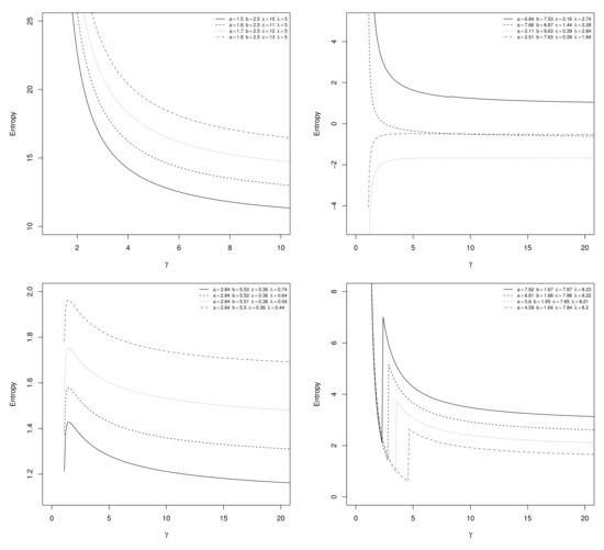
Figure 7. Plots of the Rényi entropy of the Sec-Kum-W distribution as functions of $\gamma$ for selected parameter values.

Figure 7 reveals a wide panel of shapes for the Rényi entropy of the Sec-Kum-W distribution, illustrating an undeniable entropy flexibility.

3.5. Order Statistics

Order statistics can be used in a variety of mathematical theories and applications. Here, we look at some of the distributional properties of the $i^{th}$ order statistic from the Sec-G class. Let $X_1,\dots ,X_n$ be n random variables from a random sample of the Sec-G class. Then, the PDF of the $i^{th}$ order statistic, say $X_{i:n}$, is given by

$$\begin{array}{c}\hfill h_{i:n}(x;\zeta )=i\left(\genfrac{}{}{0pt}{}{n}{i}\right)h(x;\zeta )H{(x;\zeta )}^{i-1}{\left. [1-H(x;\zeta )\right]}^{n-i},x\in \mathbb{R}.\end{array}$$

That is, in an expanded form, we have

$$\begin{array}{cc}\hfill h_{i:n}(x;\zeta )& =i\left(\genfrac{}{}{0pt}{}{n}{i}\right)\frac{\pi }{3}g(x;\zeta )sec\left({\displaystyle \frac{\pi }{3}}G(x;\zeta )\right)tan\left({\displaystyle \frac{\pi }{3}}G(x;\zeta )\right){\left. [sec\left(\frac{\pi }{3}G(x;\zeta )\right)-1\right]}^{i-1}\times \hfill \\ \hfill & {\left. [2-sec\left(\frac{\pi }{3}G(x;\zeta )\right)\right]}^{n-i},x\in \mathbb{R}.\hfill \end{array}$$

It follows from the binomial formula applied two times that

$$\begin{array}{cc}\hfill h_{i:n}(x;\zeta )& =\sum _{k=0}^{i-1}\sum _{\ell =0}^{n-i}{b}_{k,\ell }g(x;\zeta )tan\left({\displaystyle \frac{\pi }{3}}G(x;\zeta )\right)sec{\left(\frac{\pi }{3}G(x;\zeta )\right)}^{k+\ell +1},x\in \mathbb{R},\hfill \end{array}$$

where $b_{k,\ell }=(\pi /3)i\left(\genfrac{}{}{0pt}{}{n}{i}\right)\left(\genfrac{}{}{0pt}{}{i-1}{k}\right)\left(\genfrac{}{}{0pt}{}{n-i}{\ell }\right){(-1)}^{i-1-k+\ell }{2}^{n-i-\ell }$.

As a result, for any function $\psi \left(x\right)$ providing that the coming integral term exists, we have

$$\begin{array}{cc}\hfill E\left[\psi \left(X_{i:n}\right)\right]& ={\int }_{\mathbb{R}}\psi \left(x\right)h_{i:n}(x;\zeta )dx\hfill \\ \hfill & =\sum _{k=0}^{i-1}\sum _{\ell =0}^{n-i}{b}_{k,\ell }{\int }_{\mathbb{R}}\psi \left(x\right)g(x;\zeta )tan\left({\displaystyle \frac{\pi }{3}}G(x;\zeta )\right)sec{\left(\frac{\pi }{3}G(x;\zeta )\right)}^{k+\ell +1}dx.\hfill \end{array}$$

In most cases, the integral term can be calculated numerically by the use of mathematical software. This is the case for all the functions $\psi \left(x\right)$ listed in Table 1 and the setting of the Sec-Kum-W distribution. In Figure 8, we plotted the PDFs of the order statistics for a sample of size $n=5$ from a Sec-Kum-W distribution with the parameters equal to $a=1$, $b=1$, $c=1$ and $\lambda =1$.

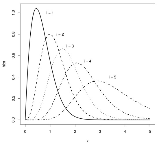
Figure 8. Plots of PDFs of order statistics for a sample of size $n=5$ of the Sec-Kum-W distribution, with parameters $a=1$, $b=1$, $c=1$ and $\lambda =1$.

From Figure 8, we see that the value of i mainly affects the skewness and kurtosis nature of the distributions.

3.6. Maximum Likelihood Method

Let $\zeta =({\zeta }_1,\dots ,{\zeta }_p)$ be a vector with p parameters and $x=(x_1,\cdots ,x_n)$ be a vector of n values from the Sec-G class. Then, we can estimate $\zeta$ by maximum likelihood method, which suggests the estimate

$$\widehat{\zeta }=argmaxL\left(\zeta \right),$$

where $L\left(\zeta \right)$ denotes the likelihood function defined as

$$\begin{array}{cc}\hfill L\left(\zeta \right)& =\prod _{i=1}^{n}h(x_i;\zeta )={\left(\frac{\pi }{3}\right)}^n\left\{\prod _{i=1}^{n}g(x_i;\zeta )\right\}\left\{\prod _{i=1}^{n}sec\left({\displaystyle \frac{\pi }{3}}G(x_i;\zeta )\right)\right\}\left\{\prod _{i=1}^{n}tan\left({\displaystyle \frac{\pi }{3}}G(x_i;\zeta )\right)\right\}.\hfill \end{array}$$

Thus defined, $\widehat{\zeta }$ is called the maximum likelihood estimate (MLE) of $\zeta$. We also have $\widehat{\zeta }=argmax\ell \left(\zeta \right)$, where $\ell \left(\zeta \right)$ denotes the log-likelihood function defined as $\ell \left(\zeta \right)=log\left[L\right(\zeta \left)\right]$, i.e.,

$$\begin{array}{cc}\hfill \ell \left(\zeta \right)& =nlog\left(\frac{\pi }{3}\right)+\sum _{i=1}^{n}log\left[g(x_i;\zeta )\right]+\sum _{i=1}^{n}log\left. [sec\left({\displaystyle \frac{\pi }{3}}G(x_i;\zeta )\right)\right]+\prod _{i=1}^{n}log\left. [tan\left({\displaystyle \frac{\pi }{3}}G(x_i;\zeta )\right)\right].\hfill \end{array}$$

Assuming that $\ell \left(\zeta \right)$ is differentiable with respect to $\zeta$, $\widehat{\zeta }$ is the simultaneous solution of the following non-linear equations: $\partial \ell \left(\zeta \right)/\partial {\zeta }_j=0$, for $j=1,\dots ,p$, with

$$\begin{array}{cc}\hfill \frac{\partial \ell \left(\zeta \right)}{\partial {\zeta }_j}& =\sum _{i=1}^n\frac{\partial g(x_i;\zeta )}{\partial {\zeta }_j}\frac{1}{g(x_i;\zeta )}+\frac{\pi }{3}\sum _{i=1}^n\frac{\partial G(x_i;\zeta )}{\partial {\zeta }_j}tan\left({\displaystyle \frac{\pi }{3}}G(x_i;\zeta )\right)\hfill \\ \hfill & +\frac{\pi }{3}\sum _{i=1}^n\frac{\partial G(x_i;\zeta )}{\partial {\zeta }_j}\frac{{\left. [sec\left({\displaystyle \frac{\pi }{3}}G(x_i;\zeta )\right)\right]}^2}{tan\left({\displaystyle \frac{\pi }{3}}G(x_i;\zeta )\right)}.\hfill \end{array}$$

Under some well-known regularity conditions, the asymptotic distribution of $\widehat{\zeta }-\zeta$ can be approximated by a well-identified multivariate normal distribution (with covariance matrix defined from the observed Fisher information matrix). Then, from this result, we can construct approximate confidence intervals as well as likelihood ratio tests. More basically, we can derive the estimated PDF by the substitution technique; $f(x;\widehat{z}eta)$ is an estimated function of $f(x;\zeta )$. The same idea can be applied to any other functions of the Sec-Kum-W distribution.

In the context of the Sec-Kum-W distribution, the expression of $(\partial g(x_i;\zeta )/\partial {\zeta }_j)(1/g(x_i;\zeta ))$ can be found in Equations (27)–(30) of [23].

4. Numerical Study

Here, we turn out the Sec-Kum-W distribution as a statistical model, and illustrate its applicability with simulated data and real-life data.

4.1. Simulation

First, we operate a simulation study to show the efficiency of the MLEs of the Sec-Kum-W model parameters. To this aim, the seckw R package is used, developed by [33]. The parameter configuration is: $a=0.3$, $b=2.2$, $c=0.15$ and $\lambda =0.05$. We choose samples of moderate sizes, between 1 and 250, and we run 1000 replicas for each sample size. Figure 9, Figure 10, Figure 11 and Figure 12 show the biases and mean squared errors (MSEs) for a, b, c and $\lambda$ considered as functions of n, respectively.

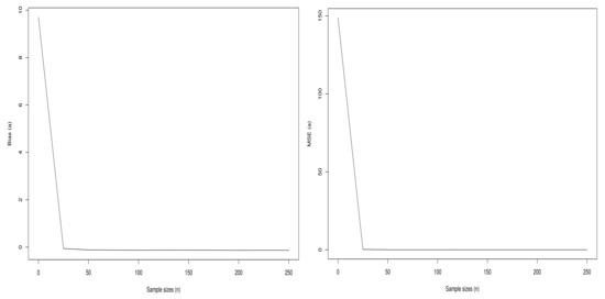
Figure 9. Plots of the biases and MSEs of the parameter a of the Sec-Kum-W distribution.

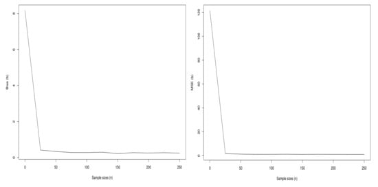
Figure 10. Plots of the biases and MSEs of the parameter b of the Sec-Kum-W distribution.

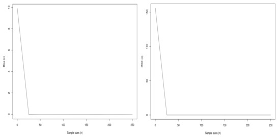
Figure 11. Plots of the biases and MSEs of the parameter c of the Sec-Kum-W distribution.

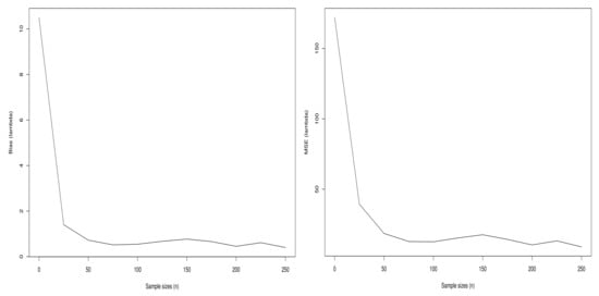
Figure 12. Plots of the biases and MSEs of the parameter $\lambda$ of the Sec-Kum-W distribution.

From Figure 9, Figure 10, Figure 11 and Figure 12, we observe that the curves of the bias tend to 0 when n increases. In addition, as anticipated, the curves of the MSEs decrease to 0 when n increases.

Table 2 summarizes the simulation results, given the means of MLEs, biases and MSEs for $n=25$, 50 and 250.

Table 2. Values of the MLEs, biases and MSEs for the parameters of the Sec-Kum-W distribution taken at $a=0.3$, $b=2.2$, $c=0.15$, and $\lambda =0.05$.

Sample Size (n)	Parameters	MLEs	Biases	MSEs
25	a	0.2403	−0.0597	0.2554
	b	2.6175	0.4175	1.7041
	c	0.1230	−0.0270	0.0179
	$\lambda$	1.4511	1.4011	39.5084
50	a	0.1843	−0.1157	0.0371
	b	2.5378	0.3378	1.3015
	c	0.1084	−0.0416	0.0139
	$\lambda$	0.7695	0.7195	18.6445
250	a	0.1694	−0.1306	0.0268
	b	2.4463	0.2463	1.0778
	c	0.1063	−0.0437	0.0122
	$\lambda$	0.4470	0.3970	9.0962

Table 2 is just a numerical illustration of what we have observed in Figure 9, Figure 10, Figure 11 and Figure 12; both biases and MSEs tend to 0 when n increases. It is expected to have lower values for these biases and MSEs for greater values of n, such as $n=1000$ or 5000.

4.2. Real-Life Data Analysis

A real-life data analysis via the Sec-Kum-W model is now being considered. Three different datasets showing diverse characteristics are used.

4.2.1. Data: Lifetime of Devices

The considered data are from [34] and represent the lifetimes of 50 devices. They are collected in Table 3.

Table 3. Lifetime of 50 devices.

0.1	0.2	1	1	1	1	1	2	3	6
7	11	12	18	18	18	18	18	21	32
36	40	45	46	47	50	55	60	63	63
67	67	67	67	72	75	79	82	82	83
84	84	84	85	85	85	85	85	86	86

Some descriptive statistics about the data are provided in Table 4.

Table 4. Descriptive statistics for the lifetime of devices.

Min.	First Quart.	Median	Mean	Third Quart.	Max.	Var.
0.10	13.50	48.50	45.69	81.25	86.00	1078.153

Then, we compare the quality of the Sec-Kum-W model fit with those of the Kumaraswamy-Weibull geometric (Kum-WG) model proposed by [28], Kumaraswamy-Weibull Poisson (Kum-WP) model introduced by [35], Kum-W model proposed by [23], Kumaraswamy Burr XII (Kum-BXII) model created by [36], and, when of interest, the simple Weibull (W) model (see [26]). For all of them, the maximum likelihood method is used to estimate the model parameters. In order to compare the fit, we consider the following criteria: Akaike information criterion (AIC), Bayesian information criterion (BIC), consistent Akaike information criterion (CAIC), and Hannan–Quinn information criterion (HQIC). The model with minimum values for these criteria may be considered as the best model to fit the data. The numerical results are collected in Table 5.

Table 5. MLEs of the parameters of the Sec-Kum-W, Kum-WG, Kum-WP, Kum-W, and Kum-BXII models with standard errors in parentheses, and AIC, BIC, CAIC, and HQIC values for the lifetimes of devices.

Distributions	Estimates					AIC	BIC	CAIC	HQIC
Sec-Kum-W$(a,b,c,\lambda )$	0.38	0.41	0.70	0.13	(-)	422.52	430.17	423.41	425.43
	(0.14)	(0.03)	(0.04)	(0.00)	(-)
Kum-WG$(a,b,c,\lambda ,p)$	0.07	0.31	5.26	0.02	0.44	455.20	464.76	456.56	458.84
	(0.02)	(0.09)	(0.15)	(0.00)	(0.40)
Kum-WP$(a,b,c,\lambda ,\beta )$	0.06	0.17	5.29	0.44	0.02	455.66	465.22	457.02	459.30
	(0.02)	(0.06)	(0.02)	(1.31)	(0.00)
Kum-W$(a,b,c,\lambda )$	0.07	0.31	4.06	0.02	(-)	456.89	464.54	457.78	459.81
	(0.03)	(0.12)	(0.73)	(0.00)	(-)
Kum-BXII$(a,b,c,k,s)$	0.08	0.31	3.90	187.24	214.27	458.92	468.48	460.28	462.56
	(0.02)	(0.08)	(0.42)	(15.24)	(10.83)

We can see that the Sec-Kum-W model, when compared to the others, proved to get the minimum values for the considered criteria. Thus, we conclude that the Sec-Kum-W distribution is quite flexible in the modeling of the proposed data. In order to visualize the obtained fit, Figure 13 displays the plots of the estimated PDFs of the considered models.

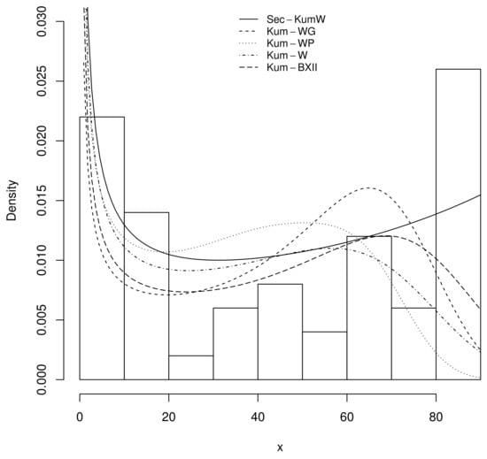
Figure 13. Plots of the estimated fitted PDFs, including one of the Sec-Kum-W model (solid line) for the lifetimes of devices.

In Figure 13, we observe an excellent fit to the data for the estimated probability functions of the Sec-Kum-W distribution; the corresponding estimated PDF fits well with the histogram of the data.

4.2.2. Data: Failure Data of 6061-T6 Aluminum

The second dataset is given by [37] on the fatigue life of 6061-T6 aluminum coupons cut parallel to the direction of rolling and oscillated at 18 cycles per second. The dataset Table 6 consists of 101 observations with maximum stress per cycle 31,000 psi.

Table 6. Failure data of 6061-T6 aluminum.

70	90	96	97	99	100	103	104	104	105	107	108	108	108	109	109	112
112	113	114	114	114	116	119	120	120	120	121	121	123	124	124	124	124
124	128	128	129	129	130	130	130	131	131	131	131	131	132	132	132	133
134	134	134	134	136	136	137	138	138	138	139	139	141	141	142	142	142
142	142	142	144	144	145	146	148	148	149	151	151	152	155	156	157	157
157	157	158	159	162	163	163	164	166	166	168	170	174	201	212

We adopt the same methodology as that developed in Section 4.2.1. First, some descriptive statistics about the data are provided in Table 7.

Table 7. Descriptive statistics for the failure data of 6061-T6 aluminum.

Min.	First Quart.	Median	Mean	Third Quart.	Max.	Var.
70.0	120.0	132.5	133.8	146.5	212.0	511.4

A simple histogram analysis shows that the data are almost symmetrical, which is a case covered by the Sec-Kum-W distribution, as shown in Figure 1. The MLEs of the parameters of the considered models, along with the AIC, BIC, CAIC, and HQIC values, are given in Table 8.

Table 8. MLEs of the parameters of the Sec-Kum-W, Kum-WP, Kum-WG, Kum-W, and Kum-BXII models with standard errors in parentheses, and AIC, BIC, CAIC, and HQIC values for the failure data of 6061-T6 aluminum.

Distributions	Estimates					AIC	BIC	CAIC	HQIC
Sec-Kum-W$(a,b,c,\lambda )$	14.48	10.54	0.97	0.02	(-)	912.59	923.01	913.01	916.80
	(1.39)	(0.59)	(0.01)	(0.00)	(-)
Kum-WP$(a,b,c,\lambda ,\beta )$	1.04	5.62	6.69	1.63	(0.01)	923.09	936.11	923.72	928.36
	(1.18)	(8.75)	(9.47)	(7.58)	(0.00)
Kum-WG$(a,b,c,\lambda ,p)$	2.18	7.17	2.98	0.01	0.25	927.64	940.67	928.28	932.91
	(0.53)	(5.02)	(1.00)	(0.00)	(1.12)
Kum-W$(a,b,c,\lambda )$	0.86	14.59	6.63	0.02	(0.00)	927.83	938.26	928.26	932.06
	(0.23)	(7.23)	(1.29)	(0.00)	(0.00)
Kum-BXII$(a,b,c,k,s)$	23.36	19.61	4.45	0.27	24.49	944.44	957.47	945.07	949.71
	(8.87)	(4.46)	(0.57)	(0.03)	(6.68)

The obtained values of the AIC, BIC, CAIC, and HQIC statistics reveal that the Sec-Kum-W is the best model in terms of fitting behavior. This can be observed in a more direct manner in Figure 14, where the estimated PDFs of the considered models are plotted.

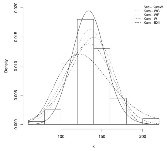
Figure 14. Plots of the estimated fitted PDFs, including one of the Sec-Kum-W model (solid line) for the failure data of 6061-T6 aluminum.

In Figure 14, we see that the estimated PDF of the Sec-Kum-W model has captured the symmetric shape of the histogram, including its upper stick. This is not the case for the competitors.

4.2.3. Data: Sums of Skin Folds

As a third data set [38], data from 100 Australian female athletes were collected at the Australian Institute of Sport (AIS). We consider the data sum of skin folds for athletes in Table 9.

Table 9. Sums of skin folds.

33.8	36.8	38.2	41.1	41.6	42.3	43.5	43.5	46.1	46.2
46.3	47.5	47.6	48.4	49.0	49.9	50.0	52.5	52.6	54.6
54.6	55.6	56.8	57.9	58.9	59.4	61.9	62.6	62.9	65.1
67.0	68.3	68.9	69.9	70.0	71.3	71.6	73.9	74.7	74.9
75.1	75.2	76.2	76.8	77.0	80.1	80.3	80.3	80.3	80.6
83.0	87.2	88.2	89.0	90.2	90.4	91.0	91.2	95.4	96.8
97.2	97.9	98.0	98.1	98.3	98.5	99.8	99.9	101.1	102.8
102.8	103.6	103.6	104.6	106.9	109.0	109.1	109.5	109.6	110.2
110.7	111.1	113.5	114.0	115.9	117.8	122.1	123.6	125.9	126.4
126.4	131.9	136.3	143.5	148.9	156.6	156.6	171.1	181.7	200.8

Again, we adopt the same methodology as that developed in Section 4.2.1. Some descriptive statistics about the data are provided in Table 10.

Table 10. Descriptive statistics for the sums of skin folds.

Min.	First Quart.	Median	Mean	Third Quart.	Max.	Var.
33.8	59.3	81.8	86.9	107.4	200.8	1145.9

A histogram analysis shows that the data are moderately right skewed, which is a case covered by the Sec-Kum-W distribution, as shown in Figure 1. The MLEs of the parameters of the considered models, along with the AIC, BIC, CAIC and HQIC values, are given in Table 10.

From Table 11, we see that the Sec-Kum-W model is the best; it has the smallest AIC, BIC, CAIC, and HQIC values. Thus, the Sec-Kum-W model presents a good fit to the data. We illustrate this claim in Figure 15.

Table 11. MLEs of the parameters of the Sec-Kum-W, Kum-WG, Kum-WP, Kum-BXII, and W models with standard errors in parentheses, and AIC, BIC, CAIC, and HQIC values for the sums of skin folds.

Distributions	Estimates					AIC	BIC	CAIC	HQIC
Sec-Kum-W$(a,b,c,\lambda )$	3.42	1.19	1.35	0.02	(-)	969.26	979.68	969.67	973.48
	(0.97)	(0.22)	(0.16)	(0.00)	(-)
Kum-WG$(a,b,c,\lambda ,p)$	3.95	0.58	2.23	0.01	0.74	983.40	996.43	984.04	988.67
	(1.57)	(0.67)	(0.59)	(0.01)	(0.15)
Kum-BXII$(a,b,c,k,s)$	13.79	10.25	1.46	0.72	16.71	984.90	997.93	985.54	990.17
	(43.23)	(8.68)	(2.19)	(1.43)	(20.14)
W$(\alpha ,\lambda )$	2.78	0.01	(-)	(-)	(-)	986.22	991.43	986.34	988.33
	(0.21)	(0.00)	(-)	(-)	(-)
Kum-WP$(a,b,c,\lambda ,\beta )$	1.72	0.66	2.32	0.83	0.01	986.40	999.43	987.04	991.67
	(0.71)	(0.44)	(0.59)	(1.45)	(0.00)

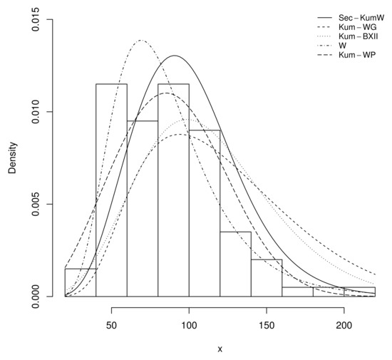
Figure 15. Plots of the estimated fitted PDFs, including one of the Sec-Kum-W model (solid line) for the sums of skin folds.

From Figure 15, we see that the estimated PDF of the Sec-Kum-W distribution has captured the form of the histogram in a better manner than those of the competitor models.

5. Concluding Remarks

In this study, we introduced a new class of distributions, with properties based on the secant function. It is called the Sec-G class. The idea is to use the functionality of the secant function to create new trigonometric distributions based on baseline distributions. It is proved that the new class first-order stochastically dominates its corresponding baseline distribution, opening new horizons of modeling. Within this class, a new trigonometric distribution, the Sec-Kum-W distribution, has been thoroughly investigated. Here, we obtained the corresponding cumulative distribution and probability density functions and their expansions, and provide discussions of various types of moments and related functions. Moreover, the model parameters were checked via maximum likelihood estimation. We applied the new distribution to three real datasets: a lifetime of devices dataset, failure data of the 6061-T6 aluminum dataset, and a sum of the skin folds dataset. It is proved that the proposed secant Kumaraswamy-Weibull model outperforms important competitors, including the Kumaraswamy-Weibull, Kumaraswamy-Weibull geometric, Kumaraswamy-Weibull Poisson, Kumaraswamy Burr XII, and Weibull models. Hence, the practical part brought evidence that the proposed model can help in the analysis of survival data, material fatigue, among others, and we conjectured that it can also be applied to other areas of knowledge.

References

- Gupta, R.D.; Kundu, D. Exponentiated exponential family: An alternative to Gamma and Weibull distributions. Biom. J. 2001, 43, 117–130. [Google Scholar] [CrossRef]
- Cordeiro, G.M.; de Castro, M. A new family of generalized distributions. J. Stat. Comput. Simul. 2021, 81, 883–898. [Google Scholar] [CrossRef]
- Marshall, A.; Olkin, I. A new method for adding a parameter to a family of distributions with applications to the exponential and Weibull families. Biometrika 1997, 84, 641–652. [Google Scholar] [CrossRef]
- Eugene, N.; Lee, C.; Famoye, F. Beta-normal distribution and its applications. Commun. Stat. Theory Methods 2002, 31, 497–512. [Google Scholar] [CrossRef]
- Zografos, K.; Balakrishnan, N. On families of beta- and generalized gamma-generated distributions and associated inference. Stat. Methodol. 2009, 6, 344–362. [Google Scholar] [CrossRef]
- Brito, C.R.; Rêgo, L.C.; Oliveira, W.R.; Gomes-Silva, F. Method for generating distributions and classes of probability distributions: The univariate case. Hacet. J. Math. Stat. 2019, 48, 897–930. [Google Scholar]
- Gilbert, G.K. The Moon’s Face: A Study of the Origin of Its Features; Bulletin of the Philosophical Society of Washington: Washington, DC, USA, 1895; Volume 12, pp. 241–292. [Google Scholar]
- Burr, I.W. Cumulative frequency functions. Ann. Math. Stat. 1942, 13, 215–232. [Google Scholar] [CrossRef]
- Raab, D. A cosine approximation to the normal distribution. Psychometrika 1961, 26, 447–450. [Google Scholar] [CrossRef]
- Nadarajah, S.; Gupta, A. The beta Fréchet distribution. Far East J. Theor. Stat. 2004, 14, 15–24. [Google Scholar]
- Lark, R.M. Modelling complex geological circular data with the projected normal distribution and mixtures of von Mises distributions. Solid Earth 2014, 5, 631–639. [Google Scholar] [CrossRef] [Green Version]
- Kumar, D.; Singh, U.; Singh, S.K. A new distribution using sine function: Its application to bladder cancer patients data. J. Stat. Appl. Probab. 2015, 4, 417–427. [Google Scholar]
- Souza, L. New Trigonometric Classes of Probabilistic Distributions. Ph.D. Thesis, Universidade Federal Rural de Pernambuco, Recife, Brazil, 2015. [Google Scholar]
- Souza, L.; Junior, W.R.O.; de Brito, C.C.R.; Chesneau, C.; Ferreira, T.A.E.; Soares, L. On the Sin-G class of distributions: Theory, model and application. J. Math. Model. 2019, 7, 357–379. [Google Scholar]
- Souza, L.; Junior, W.R.O.; de Brito, C.C.R.; Chesneau, C.; Ferreira, T.A.E.; Soares, L. General properties for the Cos-G class of distributions with applications. Eurasian Bull. Math. 2019, 2, 63–79. [Google Scholar]
- Mahmood, Z.; Chesneau, C.; Tahir, M.H. A new sine-G family of distributions: Properties and applications. Bull. Comput. Appl. Math. 2019, 7, 53–81. [Google Scholar]
- Chesneau, C.; Bakouch, H.S.; Hussain, T. A new class of probability distributions via cosine and sine functions with applications. Commun. Stat. Simul. Comput. 2019, 48, 2287–2300. [Google Scholar] [CrossRef]
- Jamal, F.; Chesneau, C. A new family of polyno-expo-trigonometric distributions with applications. Infin. Dimens. Anal. Quantum Probab. Relat. Top. 2020, 22, 1950027. [Google Scholar] [CrossRef] [Green Version]
- Jamal, F.; Chesneau, C.; Bouali, D.L.; Ul Hassan, M. Beyond the Sin-G family: The transformed Sin-G family. PLoS ONE 2021, 16, e0250790. [Google Scholar] [CrossRef] [PubMed]
- Chesneau, C.; Artault, A. On a comparative study on some trigonometric classes of distributions by the analysis of practical datasets. J. Nonlinear Model. Anal. 2021, 3, 225–262. [Google Scholar]
- Alzaatreh, A.; Lee, C.; Famoye, F. A new method for generating families of continuous distributions. Metron 2013, 71, 63–79. [Google Scholar] [CrossRef] [Green Version]
- Brito, C.C.R. Método Gerador de Distribuicoes e Classes de Distribuicoes Probabilisticas. Ph.D. Thesis, Universidade Federal Rural de Pernambuco, Recife, Brazil, 2014; p. 244. [Google Scholar]
- Cordeiro, G.M.; Ortega, E.M.M.; Nadarajah, S. The Kumaraswamy-Weibull distribution with application to failure data. J. Frankl. Inst. 2010, 349, 1399–1429. [Google Scholar] [CrossRef]
- MacGillivray, H.L. Skewness and asymmetry: Measures and orderings. Ann. Stat. 1986, 14, 994–1011. [Google Scholar] [CrossRef]
- Moors, J.J. A quantile alternative for kurtosis. J. R. Stat. Soc. Ser. D 1988, 37, 25–32. [Google Scholar] [CrossRef] [Green Version]
- Murthy, D.N.P.; Xie, M.; Jiag, R. Weibull Models; John Wiley and Sons, Inc.: Hoboken, NI, USA, 2004. [Google Scholar]
- Eissa, F.H. The Exponentiated Kumaraswamy-Weibull distribution with application to real data. Int. J. Stat. Probab. 2017, 6, 167–182. [Google Scholar] [CrossRef]
- Rasekhi, M.; Alizadeh, M.; Hamedani, G.G. The Kumaraswamy-Weibull geometric distribution with applications. Pak. J. Stat. Oper. Res. 2018, 14, 1–21. [Google Scholar] [CrossRef] [Green Version]
- Mead, M.E.; Afify, A.; Butt, N.S. The Modified Kumaraswamy-Weibull Distribution: Properties and Applications in Reliability and Engineering Sciences. Pak. J. Stat. Oper. Res. 2020, 16, 433–446. [Google Scholar] [CrossRef]
- Weisstein, E.W. Secant, From MathWorld—A Wolfram Web Resource. 2020. Available online: http://mathworld.wolfram.com/Secant.html (accessed on 19 September 2020).
- Kotz, S.; Lumelskii, Y.; Penskey, M. The Stress-Strength Model and Its Generalizations and Applications; World Scientific: Singapore, 2003. [Google Scholar]
- Rényi, A. On measures of entropy and information. In Proceedings of the 4th Berkeley Symposium on Mathematical Statistics and Probability; University of California Press: Berkeley, CA, USA, 1961; Volume 1, pp. 547–561. [Google Scholar]
- Souza, L.; Gallindo, L.; de Souza, L.S. SecKW: The SecKW Distribution. R Package Version 0.2. 2016. Available online: https://CRAN.R-project.org/package=SecKW (accessed on 21 October 2019).
- Aarset, M.V. How to identify bathtub hazard rate. IEEE Trans. Reliab. 1987, 36, 106–108. [Google Scholar] [CrossRef]
- Ramos, M.W.A.; Marinho, P.R.D.; Cordeiro, G.M.; Silva, R.V.; Hamedani, G. The Kumaraswamy-G Poisson family of distributions. J. Stat. Theory Appl. 2015, 14, 222–239. [Google Scholar] [CrossRef] [Green Version]
- Paranaiba, P.F.; Ortega, E.M.M.; Cordeiro, G.M.; Pascoa, M.A.R. The Kumaraswamy Burr XII distribution: Theory and practice. J. Stat. Comput. Simul. 2013, 83, 2117–2143. [Google Scholar] [CrossRef]
- Birnbaum, Z.W.; Saunders, S.C. Estimation for a family of life distributions with applications to fatigue. Appl. Probab. 1969, 6, 328–347. [Google Scholar] [CrossRef]
- Cook, R.; Weisberg, S. An Introduction to Regression Graphics; John Wiley & Sons: New York, NY, USA, 1994. [Google Scholar]
Publisher’s Note: MDPI stays neutral with regard to jurisdictional claims in published maps and institutional affiliations. |
© 2022 by the authors. Licensee MDPI, Basel, Switzerland. This article is an open access article distributed under the terms and conditions of the Creative Commons Attribution (CC BY) license (https://creativecommons.org/licenses/by/4.0/).