Integrability and Limit Cycles via First Integrals

Abstract

In many problems appearing in applied mathematics in the nonlinear ordinary differential systems, as in physics, chemist, economics, etc., if we have a differential system on a manifold of dimension, two of them having a first integral, then its phase portrait is completely determined. While the existence of first integrals for differential systems on manifolds of a dimension higher than two allows to reduce the dimension of the space in as many dimensions as independent first integrals we have. Hence, to know first integrals is important, but the following question appears: Given a differential system, how to know if it has a first integral? The symmetries of many differential systems force the existence of first integrals. This paper has two main objectives. First, we study how to compute first integrals for polynomial differential systems using the so-called Darboux theory of integrability. Furthermore, second, we show how to use the existence of first integrals for finding limit cycles in piecewise differential systems.

1. Introduction to the Darboux Theory of Integrability

For a differential system on a two dimensional manifold, its phase portrait is determined by the existence of a first integral. The Hamiltonian differential systems are the easiest differential systems having a first integral.

A differential system of the form:

$$\dot{x}=\frac{\partial H}{\partial y},\dot{y}=-\frac{\partial H}{\partial x},$$

where $H:{\mathbb{R}}^2\to \mathbb{R}$ is a $C^2$ function, is a Hamiltonian differential system or a simple Hamiltonian system in ${\mathbb{R}}^2$.

The integrable planar differential systems different from the Hamiltonian ones, in general, are not easy to find. First, we stated the basic results of the Darbouxian theory of integrability for finding first integrals for planar polynomial differential systems. The Darbouxian theory of integrability connects the integrability of polynomial differential systems with the invariant algebraic curves that those systems have.

1.1. Polynomial Differential Systems

Let P and Q be real polynomials in the real variables x and y. Then, a differential system:

$$\begin{array}{c}\hfill \frac{dx}{dt}=\dot{x}=P(x,y),\frac{dy}{dt}=\dot{y}=Q(x,y),\end{array}$$

(1)

is a two dimensional planar polynomial differential system or simply a polynomial system. As usual, $m=max\{degP,degQ\}$ is the degree of the polynomial system. In this paper, we supposed that the polynomials P and Q were coprime in the ring of real polynomials in the variables x and y.

The Darboux theory of integrability illustrates for a polynomial differential system the relationships between the existence of exact algebraic solutions (an algebraic phenomenon) and the integrability (a topological phenomenon).

1.2. First Integrals

As usual, the vector field:

$$X=P\frac{\partial }{\partial x}+Q\frac{\partial }{\partial y}$$

is associated to the differential system (1).

Let U be an open subset of ${\mathbb{R}}^2$. We stated that the polynomial differential system (1) was integrable in U if there was a non-constant analytic function $H:U\to$$\mathbb{R}$ that was constant on all orbits $\left(x\right(t),y(t\left)\right)$ of the system (1) contained in U. Such a function is called a first integral. It was clear that H is a first integral of system (1) in U if, and only if, the following equality holds:

$$\frac{dH}{dt}=H_x\dot{x}+H_y\dot{y}=H_{x}P+H_{y}Q=XH=0\mathrm{in} U.$$

Of course, the curves $H(x,y)=$ constant in U were formed by the orbits of the differential system (1).

Example 1.

Consider the Hamiltonian system:

$$\dot{x}=\frac{\partial H}{\partial y}=P,\dot{y}=-\frac{\partial H}{\partial x}=Q.$$

Then, the function H is called the Hamiltonian of this system, and H is a first integral of it, because:

$$XH=P\frac{\partial H}{\partial x}+Q\frac{\partial H}{\partial y}=H_y{H}_x-H_x{H}_y=0.$$

1.3. Integrating Factors

Again, U denotes an open subset of ${\mathbb{R}}^2$. An analytic function $R:U\to \mathbb{R}$ non-identically zero is an integrating factor of the polynomial differential system (1) in U if one of the next three equivalent conditions is satisfied in U:

$$XR=-R\mathrm{div}(P,Q),\mathrm{div}(RP,RQ)=0,\frac{\partial \left(RP\right)}{\partial x}+\frac{\partial \left(RQ\right)}{\partial y}=0.$$

As usual, we defined the divergence of the vector field $X=(P,Q)$ by:

$$\mathrm{div}\left(X\right)=\frac{\partial P}{\partial x}+\frac{\partial Q}{\partial y}=\mathrm{div}(P,Q).$$

Doing the change of time $dt=rds$, the differential system (1) becomes:

$$\dot{x}=RP=\frac{\partial H}{\partial y},\dot{y}=RQ=-\frac{\partial H}{\partial x}.$$

(2)

Note that, since system (2) has a divergence of zero, it is Hamiltonian.

To each integrating factor R, there is a first integral H associated, given by:

$$H(x,y)=\int R(x,y)P(x,y)dy+h(x),$$

(3)

and the function h must satisfy $\frac{{\displaystyle \partial H}}{{\displaystyle \partial x}}=-RQ$.

Example 2.

The quadratic polynomial differential system:

$$\dot{x}=-y-b(x^2+y^2)=P,\dot{y}=x=Q,$$

(4)

has the integrating factor $R=1/(x^2+y^2)$. Indeed,

$$\frac{\partial \left(RP\right)}{\partial x}+\frac{\partial \left(RQ\right)}{\partial y}=\frac{\partial (-y-b(x^2+y^2))/(x^2+y^2)}{\partial x}+\frac{\partial x/(x^2+y^2)}{\partial y}=0.$$

In order to find a first integral of system (4), we follow (3), i.e.,:

$$H=\int RPdy+h\left(x\right)=\int \frac{-y-b(x^2+y^2)}{x^2+y^2}dy+h\left(x\right)=-by-\frac{1}{2}log(x^2+y^2)+h\left(x\right).$$

Then,

$$\frac{{\displaystyle \partial H}}{{\displaystyle \partial x}}+RQ=h^{\prime }\left(x\right)=0.$$

Therefore, $h\left(x\right)$ is a constant and we can omit it from the first integral H; hence:

$$H=-by-\frac{1}{2}log(x^2+y^2),$$

or, as the first integral, we can take:

$$F=e^H=\frac{e^{-by}}{\sqrt{x^2+y^2}}.$$

The result of the next proposition is well known; for instance, see [1]. Since its proof is very short, we provided it.

Proposition 1.

Let $R_1$ and $R_2$ be two integrating factors of the polynomial differential system (1) in the open subset U of ${\mathbb{R}}^2$; then, the function $R_1/R_2$ is a first integral in the open set $U\backslash \{R_2=0\}$, if $R_1/R_2$ is non-constant.

Proof. 

We have $X{R}_i=-R_i\mathrm{div}(P,Q)$ because $R_i$ is an integrating factor for $i=1,2$. Therefore, from:

$$X\left(\frac{R_1}{R_2}\right)=\frac{\left(X{R}_1\right)R_2-R_1\left(X{R}_2\right)}{R_2^2}=0,$$

the proposition follows. □

1.4. Invariant Algebraic Curves

A non-constant polynomial $f\in \mathbb{R}[x,y]$ defines the invariant algebraic curve of the polynomial differential system (1) if there is a polynomial $K\in \mathbb{R}[x,y]$, such that:

$$Xf=P\frac{\partial f}{\partial x}+Q\frac{\partial f}{\partial y}=Kf.$$

(5)

We stated that the invariant algebraic curve $f=0$ has, as a cofactor, the polynomial K. Of course, the cofactor has a degree of at most $m-1$, because m is the degree of the polynomial differential system.

From (5), it follows that the gradient $(\partial f/\partial x,\partial f/\partial y)$ of the invariant algebraic curve $f=0$ is orthogonal to the vector field $X=(P,Q)$ at the points of the curve $f=0$. Therefore, at each point of the curve $f=0$, the vector X is tangent to the curve $f=0$; therefore, the curve $f=0$ is formed by orbits of the vector field X. Therefore, since the curve $f=0$ is invariant under the flow defined by X, this curve is called an “invariant algebraic curve”.

If the polynomial f was irreducible in the ring $\mathbb{R}[x,y]$, then we stated that the invariant algebraic curve $f=0$ was irreducible.

Example 3.

We claim that $f_1=ay+b=0$ with cofactor $K_1=ax$ and $f_2=x^2+y^2-1=0$ with cofactor $K_2=-2x$ are two invariant algebraic curves of the quadratic polynomial differential system:

$$\dot{x}=-y(ay+b)-(x^2+y^2-1)=P,\dot{y}=x(ay+b)=Q,$$

(6)

$a\ne 0$. Indeed,

$$X{f}_1=P\frac{\partial ay+b}{\partial x}+Q\frac{\partial ay+b}{\partial y}=x(ay+b)a=K_1{f}_1,$$

and

$$\begin{array}{cc}\hfill X{f}_2=& P{\displaystyle \frac{\partial f_2}{\partial x}}+Q{\displaystyle \frac{\partial f_2}{\partial y}}=(-y(ay+b)-(x^2+y^2-1))2x+x(ay+b)2y\hfill \\ \hfill =& -(x^2+y^2-1)2x=K_2{f}_2.\hfill \end{array}$$

1.5. Exponential Factors

Other objects playing a similar role as the invariant algebraic curves in order to obtain first integrals of a polynomial differential system (1) are the exponential factors.

Let $h,g\in \mathbb{R}[x,y]$ either be coprime polynomials in the ring $\mathbb{R}[x,y]$, or $h\equiv 1$. Then, for the polynomial differential system (1), the function $exp(g/h)$ is an exponential factor if there is a polynomial $K\in \mathbb{R}[x,y]$ of a degree of at most $m-1$, such that:

$$X\left(exp\left(\frac{g}{h}\right)\right)=Kexp\left(\frac{g}{h}\right).$$

(7)

Then, for the exponential factor $exp(g/h)$ we stated that K was its cofactor.

Since the exponential factor cannot vanish, it does not define invariant curves of the polynomial system (1).

Example 4.

Consider the polynomial differential quadratic system:

$$\dot{x}=x(y+a)=P,\dot{y}=y=Q.$$

Such a system has the exponential factor $e^y$. Indeed:

$$X{e}^y=P\frac{\partial e^y}{\partial x}+Q\frac{\partial e^y}{\partial y}=y{e}^y=K{e}^y,$$

with cofactor $K=y$.

1.6. The Method of Darboux

For polynomial differential systems (1), we summarized the Darboux theory of integrability in the next theorem.

Theorem 1.

Let $f_i=0$ be irreducible invariant algebraic curves with cofactors $K_i$ for $i=1,\dots ,p$, and let $exp(g_j/h_j)$ be exponential factors with cofactors $L_j$ for $j=1,\dots ,q$ for a polynomial differential system (1) of degree m.

(i) 

The function:

$$f_1^{{\lambda }_1}\dots f_p^{{\lambda }_p}{\left(exp\left(\frac{g_1}{h_1}\right)\right)}^{{\mu }_1}\dots {\left(exp\left(\frac{g_q}{h_q}\right)\right)}^{{\mu }_q}$$

(8)

is a first integral of system (1) if, and only if, there are ${\lambda }_i,{\mu }_j\in \mathbb{R}$, not all zero, such that: ${\displaystyle \sum _{i=1}^p}{\lambda }_i{K}_i+{\displaystyle \sum _{j=1}^q}{\mu }_j{L}_j=0$.

(ii) 

When $p+q\ge m(m+1)/2+1$, there are ${\lambda }_i,{\mu }_j\in \mathbb{R}$, not all zero, satisfying ${\displaystyle \sum _{i=1}^p}{\lambda }_i{K}_i+{\displaystyle \sum _{j=1}^q}{\mu }_j{L}_j=0$.

(iii) 

If $p+q\ge m(m+1)/2+2$, all orbits of the differential system (1) are contained in invariant algebraic curves, because the system has a rational first integral.

(iv) 

Function (8) is an integrating factor of system (1) if, and only if, there are ${\lambda }_i,{\mu }_j\in \mathbb{R}$, not all zero, such that ${\displaystyle \sum _{i=1}^p}{\lambda }_i{K}_i+{\displaystyle \sum _{j=1}^q}{\mu }_j{L}_j=-div(P,Q)$.

(v) 

We defined $F_j=exp(g_j/h_j)$. Since $f_i=0$ are invariant algebraic curves with cofactors, and $K_i$ and $F_j$ are exponential factors with cofactors $L_j$, we have $X{f}_i=K_i{f}_i$, and $X{F}_j=L_j{F}_j$. Therefore, the statement (i) follows from the equality:

$$\begin{array}{cc}\hfill X\left(f_1^{{\lambda }_1}\dots f_p^{{\lambda }_p}{F}_1^{{\mu }_1}\dots F_q^{{\mu }_q}\right)& =\hfill \\ \hfill \left(f_1^{{\lambda }_1}\dots f_p^{{\lambda }_p}{F}_1^{{\mu }_1}\dots F_q^{{\mu }_q}\right)\left(\sum _{i=1}^p{\lambda }_i\frac{X{f}_i}{f_i}+\sum _{j=1}^q{\mu }_j\frac{X{F}_j}{F_j}\right)& =\hfill \\ \hfill \left(f_1^{{\lambda }_1}\dots f_p^{{\lambda }_p}{F}_1^{{\mu }_1}\dots F_q^{{\mu }_q}\right),\left(\sum _{i=1}^p{\lambda }_i{K}_i+\sum _{j=1}^q{\mu }_j{L}_j\right)& =0.\hfill \end{array}$$

Example 5.

Assume that $a\ne 0$ in the quadratic system:

$$\dot{x}=-y(ay+b)-(x^2+y^2-1),\dot{y}=x(ay+b).$$

(9)

Then, this system has $f_2=x^2+y^2-1=0$ with cofactor $K_2=-2x$, and $f_1=ay+b=0$ with cofactor $K_1=ax$, as invariant algebraic curves. Due to the fact $2K_1+a{K}_2=0$, by Theorem 1

(i) 

We obtained that $H={(ay+b)}^2{(x^2+y^2-1)}^a$ is a first integral of system (9).

(ii) 

Since the degree of the polynomial cofactors $K_i$ and $L_j$ is at most $m-1$, we obtained that $K_i,L_j\in {\mathbb{R}}_{m-1}[x,y]$, the space of all polynomials of $\mathbb{R}[x,y]$ of a degree of at most $m-1$. We observed that the vector space ${\mathbb{C}}_{m-1}[x,y]$ over $\mathbb{C}$ has a dimension $m(m+1)/2$.

Since all the polynomials $K_i$ and $L_j$ belong to the vector space ${\mathbb{C}}_{m-1}[x,y]$ of the dimension $(m+1)/2]$, and we have $p+q$ polynomials $K_i$ and $L_j$ with $p+q>m(m+1)/2$, and we obtained that the $p+q$ polynomials must be linearly dependent in ${\mathbb{C}}_{m-1}[x,y]$. Therefore, there are ${\lambda }_i,{\mu }_j\in \mathbb{C}$, not all zero, such that ${\displaystyle \sum _{i=1}^p}{\lambda }_i{K}_i+{\displaystyle \sum _{j=1}^q}{\mu }_j{L}_j=0$. Hence, statement (ii) was proved.

Example 6.

Consider the real quadratic system:

$$\dot{x}=x(ax+c),\dot{y}=y(2ax+by+c),$$

(10)

with $abc\ne 0$. Then, this system has the following five invariant straight lines: $f_1=x=0$, $f_2=ax+c=0$, $f_3=y=0$, $f_4=ax+by=0$, $f_5=ax+by+c=0$. Therefore, from Theorem 1(ii) we obtained that system (10) has the first integral $H=f_1^{{\lambda }_1}{f}_2^{{\lambda }_2}{f}_3^{{\lambda }_3}{f}_4^{{\lambda }_4}{f}_5^{{\lambda }_5}$ with ${\lambda }_i\in \mathbb{R}$, satisfying ${\displaystyle \sum _{i=1}^5}{\lambda }_i{K}_i=0$, where $K_i$ is the cofactor of $f_i$. It is easy to check that $K_1=ax+c$, $K_2=ax$, $K_3=2ax+by+c$, $K_4=ax+by+c$, $K_5=ax+by$. Hence, a solution of ${\displaystyle \sum _{i=1}^5}{\lambda }_i{K}_i=0$ is ${\lambda }_1={\lambda }_5=-1$, ${\lambda }_2={\lambda }_4=1$ and ${\lambda }_3=0$. Therefore a first integral of system (10) is:

$$H=\frac{(ax+c)(ax+by)}{x(ax+by+c)}.$$

(iii) 

Under the hypotheses of this statement, we applied statement (ii) to the two following subsets of $p+q-1>0$ functions formed by the invariant algebraic curves and the exponential factors. In this way, we obtained two linear dependencies between their corresponding cofactors, with which, after some relabeling and linear algebra, we could obtain:

$$M_1+{\alpha }_3{M}_3+\dots +{\alpha }_{p+q-1}{M}_{p+q}=0,M_2+{\beta }_3{M}_3+\dots +{\beta }_{p+q-1}{M}_{p+q}=0,$$

where $M_l$ are the cofactors $L_j$ and $K_i$, and ${\alpha }_l,{\beta }_l\in \mathbb{R}$. Therefore, by statement (i), we obtained that the two first integrals:

$$G_1{G}_3^{{\alpha }_3}\dots G_{p+q-1}^{{\alpha }_{p+q}},G_2{G}_3^{{\beta }_3}\dots G_{p+q-1}^{{\beta }_{p+q}},$$

of the differential system (1), $G_l$ is either an invariant algebraic curve or an exponential factor with cofactor $M_l$ for $l=1,\dots ,p+q$. Therefore, taking logarithms of these two, these previous first integrals, we obtained that:

$$\begin{array}{ccc}\hfill H_1& =& log\left(G_1\right)+{\alpha }_{3}log\left(G_3\right)+\dots +{\alpha }_{p+q}log\left(G_{p+q}\right),\hfill \\ \hfill H_2& =& log\left(G_2\right)+{\beta }_{3}log\left(G_3\right)+\dots +{\beta }_{p+q}log\left(G_{p+q}\right),\hfill \end{array}$$

are also first integrals of the differential system (1) where they are defined. Each one of these first integrals has associated an integrating factor $R_i$ satisfying:

$$P=R_i\frac{\partial H_i}{\partial y},Q=-R_i\frac{\partial H_i}{\partial x}.$$

Therefore, we have that:

$$\frac{R_1}{R_2}={\displaystyle \frac{\partial H_2}{\partial x}}/{\displaystyle \frac{\partial H_1}{\partial x}}.$$

Due to the fact that the functions $G_l$ are exponentials of a quotient of polynomials, or polynomials, we obtained that $\partial H_i/\partial x$ are rational functions for $i=1,2$. Therefore, we obtained that $R_1/R_2$ is a rational function, and by Proposition 1 we know that $R_1/R_2$ is a rational first integral. Hence, statement (iii) was proved.

In Example 5, we observed that, since this system has five invariant algebraic curves, by Theorem 1(iii) it has a rational first integral. The one that we obtained.

(iv) 

Since equality ${\displaystyle \sum _{i=1}^p}{\lambda }_i{K}_i+{\displaystyle \sum _{j=1}^q}{\mu }_j{L}_j=-div(P,Q)$ is equivalent to the equality:

$$\begin{array}{cc}\hfill X\left(f_1^{{\lambda }_1}\dots f_p^{{\lambda }_p}{F}_1^{{\mu }_1}\dots F_q^{{\mu }_q}\right)& =\hfill \\ \hfill \left(f_1^{{\lambda }_1}\dots f_p^{{\lambda }_p}{F}_1^{{\mu }_1}\dots F_q^{{\mu }_q}\right)\left(\sum _{i=1}^p{\lambda }_i{K}_i+\sum _{j=1}^q{\mu }_j{L}_j\right)& =\hfill \\ \hfill -\left(f_1^{{\lambda }_1}\dots f_p^{{\lambda }_p}{F}_1^{{\mu }_1}\dots F_q^{{\mu }_q}\right)div(P,Q)& .\hfill \end{array}$$

Therefore, statement (iv) was proved.

Example 7.

The algebraic curve $f_1=x^2+y^2$ is invariant for the differential system:

$$\dot{x}=-y-b(x^2+y^2)=P,\dot{y}=x=Q,$$

(11)

with cofactor $K_1=-2bx$. Since $K_1=div(P,Q)$, we obtained from Theorem 1(iv) that $f_1^{-1}$ is an integrating factor of this differential system. Using this integrating factor, we could compute the first integral $H=exp(-2by)(x^2+y^2)$ of system (11).

The Darboux theory of integrability, here presented for polynomial differential systems in ${\mathbb{R}}^2$, was extended to polynomial differential differential systems in ${\mathbb{R}}^n$ and ${\mathbb{C}}^n$. For more information on the Darboux theory of integrability, see Chapter 8 of [2].

We must mention that there is another nice theory for finding first integrals of the ordinary differential equations using the Lie symmetries; for instance, see book [3].

2. Limit Cycles in Piecewise Differential Systems via First Integrals

The study of limit cycles is one of the most important objectives in the qualitative theory of the planar ordinary differential equations. We remark that, to obtain an upper bound for the maximum number of limit cycles for a given differential system in the plane ${\mathbb{R}}^2$, in general, is a very difficult problem.

The study of the discontinuous piecewise differential systems, more recently also called Filippov systems, has attracted the attention of mathematicians during these past decades due to their applications. These piecewise differential systems in the plane are formed by different differential systems defined in distinct regions separated by a curve. A pioneering work on this subject was due to Andronov, Vitt and Khaikin in the 1920s, and later on, Filippov, in 1988, provided the theoretical bases for these kinds of differential systems. Nowadays, a vast literature on these differential systems is available; for instance, see the books of [4,5,6,7] and the survey by [8]. As for the smooth differential systems, the study of the existence and location of limit cycles in the piecewise differential systems is also of great importance.

The main tools for computing analytical limit cycles of differential systems are based on the averaging theory, the Melnikov integral, the Poincaré map, and the Poincaré map together with the Newton–Kantorovich Theorem or the Poincaré–Miranda theorem. To these tools, in the particular case of the piecewise differential systems, we had to add the use of the first integrals of the differential systems forming the piecewise differential systems for computing their limit cycles.

To show how to use the first integrals for computing the limit cycles and the periodic orbits of the piecewise differential systems is the objective of this second part of this paper. Of course, this tool is restricted to the piecewise differential systems such that all their differential systems be integrable, in the sense that we know for each of them a further invariant st integral.

2.1. Discontinuous Piecewise Differential Systems

A discontinuous piecewise differential system on ${\mathbb{R}}^2$ is a pair of C${}^r$ (with $r\ge 1$) differential systems in ${\mathbb{R}}^2$ separated by a smooth curve $\Sigma .$ The line of discontinuity $\Sigma$ of the discontinuous piecewise differential system is given by $\Sigma =h^{-1}\left(0\right),$ where $h:{\mathbb{R}}^2⟶\mathbb{R}$ is a $C^1$ function having 0 as a regular value. Observe that $\Sigma$ is the boundary between the regions ${\Sigma }^{+}=\{(x,y)\in {\mathbb{R}}^2|h(x,y)>0\}$ and ${\Sigma }^{-}=\{(x,y)\in {\mathbb{R}}^2|h(x,y)<0\}$. Hence:

$$Z(x,y)=\left\{\begin{array}{cc}X(x,y),\hfill & \mathrm{if}h(x,y)\ge 0,\hfill \\ Y(x,y),\hfill & \mathrm{if}h(x,y)\le 0,\hfill \end{array}\right.$$

(12)

is the vector field corresponding to a piecewise differential system with a line of discontinuity $\Sigma$.

When the vector fields X and Y coincide on the line $\Sigma$, we obtain a continuous piecewise differential system on ${\mathbb{R}}^2$, that, in general, will not be smooth on $\Sigma$.

The vector field (12) is usually denoted by $Z=(X,Y,\Sigma )$ or simply by $Z=(X,Y)$, if the separation line $\Sigma$ is known. In order to establish a definition for the trajectories of Z, we had to have a criterion for the transition of the trajectories between ${\Sigma }^{+}$ and ${\Sigma }^{-}$ across the curve of discontinuity $\Sigma$. The contact between the curve of discontinuity $\Sigma$ and the vector field X (or Y) is described by the directional derivative of h with respect to the vector field X, i.e.,:

$$Xh\left(p\right)=⟨\nabla h\left(p\right),X\left(p\right)⟩.$$

Here, $⟨.,.⟩$ denotes the usual inner product of the plane ${\mathbb{R}}^2.$ Filippov in [9] stated the main results of the discontinuous piecewise differential systems. The curve of discontinuity $\Sigma$ is divided into the three following sets:

(a)

${\Sigma }^c:\{p\in \Sigma :Xh\left(\mathbf{x}\right)·Yh\left(\mathbf{x}\right)>0\}$, the Crossing set.

(b)

${\Sigma }^e:\{p\in \Sigma :Xh\left(\mathbf{x}\right)>0\mathrm{and}Yh\left(\mathbf{x}\right)<0\}$, the Escaping set.

(c)

${\Sigma }^s:\{p\in \Sigma :Xh\left(\mathbf{x}\right)<0\mathrm{and}Yh\left(\mathbf{x}\right)>0\}$, the Sliding set.

The points of $\Sigma$, where both vector fields X and Y simultaneously point outwards or inwards, define the escaping ${\Sigma }^e$ or sliding ${\Sigma }^s$ regions, while the interior in $\Sigma$ of their complement defines the crossing region ${\Sigma }^c$ (see Figure 1). The points of $\Sigma$, which are not in ${\Sigma }^c\cup {\Sigma }^e\cup {\Sigma }^s$, are the tangency points between X or Y and $\Sigma .$

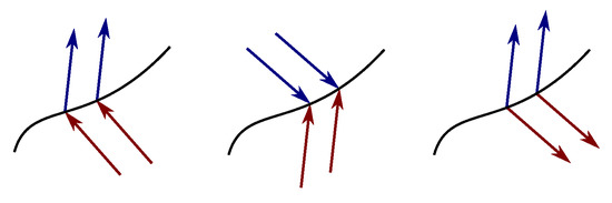
Figure 1. Crossing, sliding, and escaping regions, respectively.

There are many papers studying the limit cycles of continuous and discontinuous piecewise differential systems in ${\mathbb{R}}^2$; for instance, see [8,10,11,12,13,14,15,16,17,18,19,20,21,22,23].

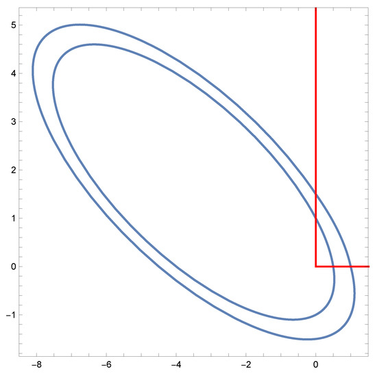
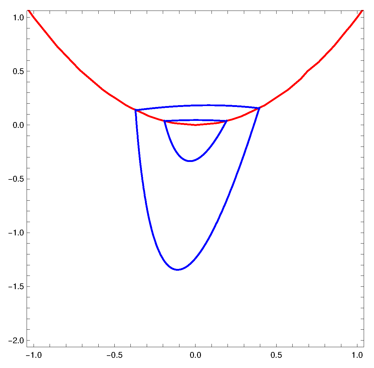
2.2. Limit Cycles of a Piecewise Differential System Formed by a Linear Differential System and a Quadratic Polynomial Differential System Separated by the Straight Line $x=0$

In what follows, we wanted to study the limit cycles of the following discontinuous piecewise differential system separated by the straight line $x=0$. In the half-plane $x\ge 0$, there is the linear differential system:

$$\dot{x}=2+2x-2y,\dot{y}=6-2y,$$

(13)

and in the half-plane $x\le 0$, there is the quadratic polynomial differential system:

$$\begin{array}{cc}\hfill \dot{x}& =-9x+15y+4x^2+8xy-28y^2,\hfill \\ \hfill \dot{y}& =-6x+9y-4x^2+32xy-44y^2.\hfill \end{array}$$

(14)

Theorem 2.

The discontinuous piecewise differential systems (13) and (14) have a unique limit cycle shown in Figure 2.

Figure 2. The unique limit cycle that exists for the piecewise differential systems (13) and (14). The limit cycle is travels in counterclockwise sense.

Proof. 

Since we wanted to compute the limit cycles of this piecewise differential system using their first integrals, we had to find such first integrals.

It is known that all the linear differential systems in ${\mathbb{R}}^n$ for $n\ge 2$ are Darboux integrable (see [24]), so, in particular, the differential system (13) must have a first integral. Clearly, the differential system (13) is Hamiltonian with Hamiltonian:

$$H_1(x,y)=6x-2y-2xy+y^2.$$

Therefore, we obtained a first integral of system (13).

System (14) has a center at the origin of coordinates, because the eigenvalues of the linear part of the system at the origin are $\pm 3i$, so the origin is either a weak focus or a center, but when computing their Lyapunov constants, we saw that all of them are zero, so it is a center; for more details, see Chapter 5 of [2]. Moreover, it is well known that all quadratic polynomial differential systems having a center are Darboux integrable; for more details see the proof of Theorem 8.15 of [2] or paper [25].

Now, in order to find a first integral for the differential system (14) we applied the Darboux theory of integrability. We started looking for their invariant algebraic curves of degrees one and two.

First, we looked for invariant straight lines $f=f(x,y)=ax+by+c=0$, and since the polynomial differential system has a degree of two, their cofactors must be polynomials of a degree of at most one, so they must be of the form $K=k_0+k_{1}x+k_{2}y$, and f and K must satisfy Equation (5). Passing the right hand side of this equation to the left, we obtained the polynomial:

$$\begin{array}{c}-c{k}_0+(-9a-6b-a{k}_0-c{k}_1)x+(15a+9b-b{k}_0-c{k}_2)y+(4a-4b-a{k}_1)x^2+\hfill \\ (8a+32b-b{k}_1-a{k}_2)xy+(-28a-44b-b{k}_2)y^2=0.\hfill \end{array}$$

Therefore, we had to solve the system:

$$\begin{array}{c}c{k}_0=0,\hfill \\ 9a+6b+a{k}_0+c{k}_1=0,\hfill \\ 15a+9b-b{k}_0-c{k}_2=0,\hfill \\ 4a-4b-a{k}_1=0,\hfill \\ 8a+32b-b{k}_1-a{k}_2=0,\hfill \\ 28a+44b+b{k}_2=0,\hfill \end{array}$$

in the unknowns $a,b,c,k_0,k_1$, and $k_2$ for obtaining the possible invariant straight lines of the differential system (14). This system has a unique solution with $(a,b,c)=(0,0,0)$. Namely, $b=-a$, $c=-3a/8$, $k_0=0$, $k_1=8$, and $k_2=-16$. Therefore, we obtained:

$$f=\frac{1}{8}a(8x-8y-3)andK=8(x-2y).$$

Therefore, without a loss of generality, we could assume that the invariant straight line is $f_1=8x-8y-3=0$ with the cofactor $K_1=8(x-2y)$.

Now, we looked for possible invariant algebraic curves of degree two. Therefore, we had to solve Equation (5) with $f=a_0+a_{1}x+a_{2}y+a_3{x}^2+a_{4}xy+a_5{y}^2$ and $K=k_0+k_{1}x+k_{2}y$. Solving it, in a similar way for obtaining the invariant algebraic curves of degree one, we obtained only two invariant algebraic curves of degrees two for one, namely:

$$-\frac{1}{128}{a}_4{(8x-8y-3)}^2=0,\mathrm{and}-\frac{1}{768}{a}_4(-9+96x-96y+128x^2-768xy+896y^2).$$

The first solution really is an invariant straight line. Therefore, essentially, there is a unique invariant algebraic curve of degree two, which we could take: $f_2=-9+96x-96y+128x^2-768xy+896y^2=0$ with cofactor $K_2=32(x-2y)$.

We knew that the equation ${\lambda }_1{K}_1+{\lambda }_2{K}_2=0$ is satisfied with ${\lambda }_1=-4$ and ${\lambda }_2=1$; therefore, by Theorem 2(ii) we obtained the first integral:

$$H_2(x,y)=\frac{-9+96x-96y+128x^2-768xy+896y^2}{{(8x-8y-3)}^4}.$$

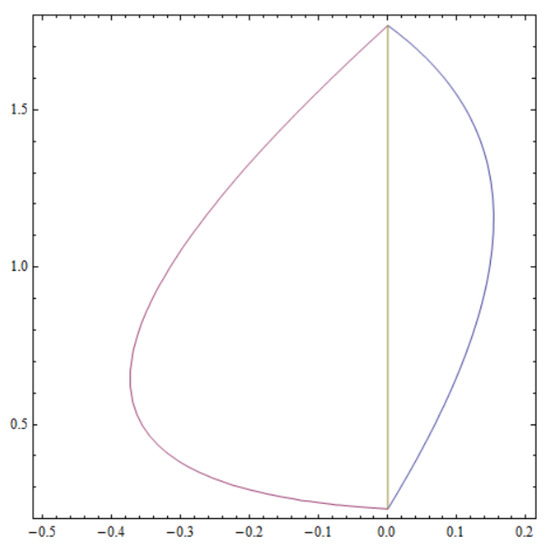
Clearly, in the half-planes $x\ge 0$ and $x\le 0$, the differential systems (13) and (14) have no limit cycles, because the polynomial $H_1$ and rational first integral $H_2$ prevent their existence, respectively. Therefore, the piecewise differential system formed with the systems (13) and (14) separated by the straight line $x=0$ has limit cycles, which must cross line $x=0$ in exactly two points, denoted by $(0,y)$ and $(0,Y)$ with $y<Y$. These two points must be crossing points and satisfy the system:

$$e_1=H_1(0,y)-H_1(0,Y)=0,e_2=H_2(0,y)-H_2(0,Y)=0.$$

The unique solution of this system satisfying $y<Y$ is:

$$(y,Y)=\frac{1}{1616}\left(1616-\sqrt{2222(1013-9\sqrt{1257})},1616+\sqrt{2222(1013-9\sqrt{1257})}\right).$$

(15)

This solution provides the limit cycle of Figure 2. □

2.3. Limit Cycles of Piecewise Differential Systems Formed by Three Linear Centers

These last years, since the piecewise linear differential systems, had many relevant applications to physical phenomena; the interest for studying them has increased strongly. As in the smooth differential systems also in the piecewise linear differential systems, the study of their limit cycles plays a main role. Almost all papers studying the limit cycles of the piecewise linear differential systems consider piecewise linear differential systems formed only by two pieces. In this subsection, we studied piecewise linear differential systems formed with three pieces.

In [26], we studied the limit cycles in ${\mathbb{R}}^2$ of the discontinuous piecewise linear differential systems separated by the line of discontinuity

$$\Sigma =\{(x,y)\in {\mathbb{R}}^2:y=0\mathrm{or}x=0\mathrm{and}y\ge 0\},$$

and formed by three arbitrary linear centers. Such discontinuous piecewise linear differential systems can exhibit, at most, three limit cycles, three being the maximum number of limit cycles that they can exhibit. In particular, it was proved that there are such piecewise linear differential systems with three limit cycles, each limit cycle having a unique point in each branch of the three branches of $\Sigma \backslash \left\{\right(0,0\left)\right\}$.

The three components of ${\mathbb{R}}^2\backslash \Sigma$ are $Q_1=\{(x,y)\in {\mathbb{R}}^2:x>0\mathrm{and}y>0\}$, $Q_2=\{(x,y)\in {\mathbb{R}}^2:x<0\mathrm{and}y>0\}$, and $H=\{(x,y)\in {\mathbb{R}}^2:y<0\}$.

The objective of this section was to study the limit cycles of the discontinuous piecewise linear differential system defined by:

$$\begin{array}{ccc}\dot{x}={\displaystyle \frac{2}{1565}}y+{\displaystyle \frac{379}{1565}},\hfill & \dot{y}=-2x+{\displaystyle \frac{237}{313}},\hfill & \mathrm{in} Q_1,\hfill \\ \dot{x}={\displaystyle \frac{4}{1565}}y+{\displaystyle \frac{11566}{10955}},\hfill & \dot{y}=-8x-{\displaystyle \frac{4\sqrt{4430533}}{2191}},\hfill & \mathrm{in} Q_2,\hfill \\ \dot{x}=2y,\hfill & \dot{y}=-8x-{\displaystyle \frac{2\left(\sqrt{4430533}-1299\right)}{2191}},\hfill & \mathrm{in} H.\hfill \end{array}$$

(16)

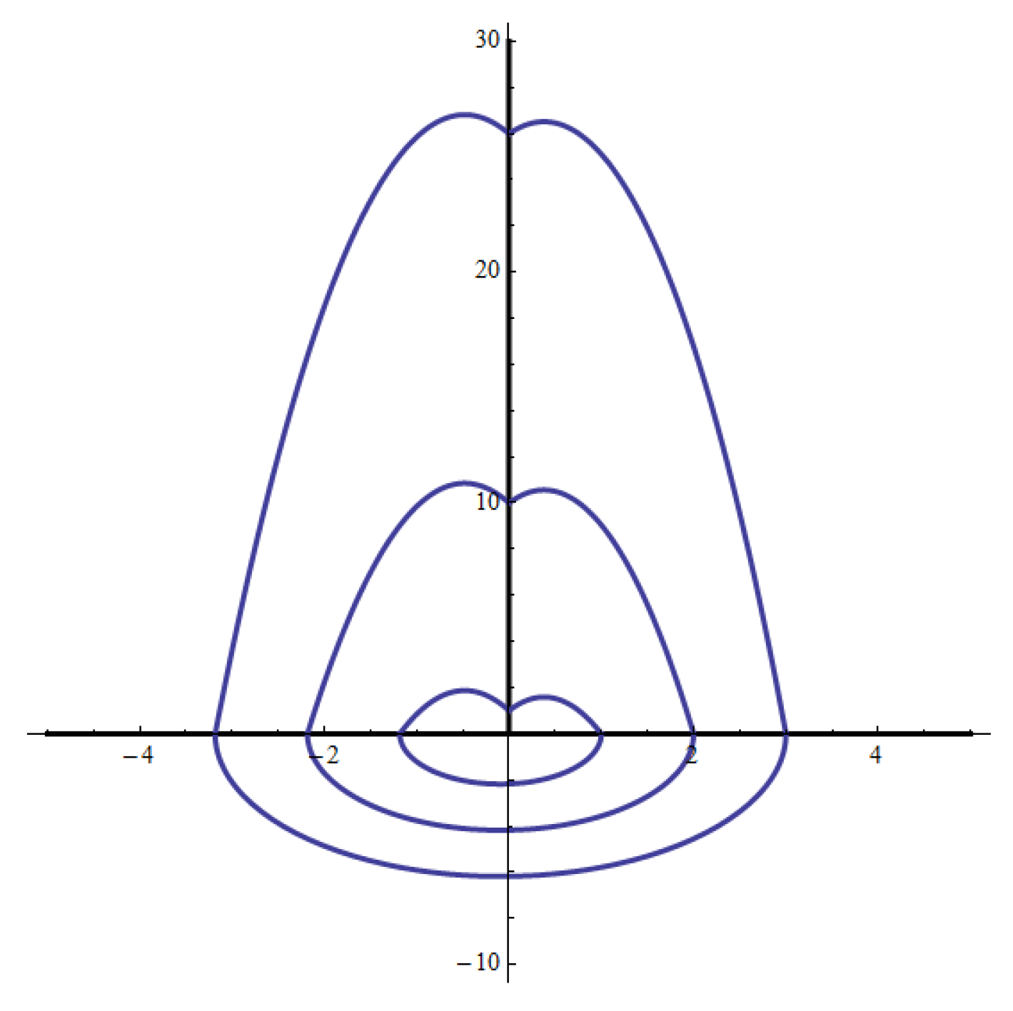
Theorem 3.

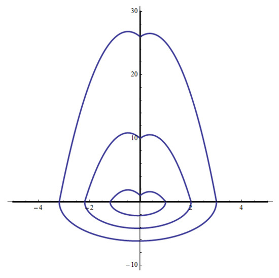
The discontinuous piecewise differential system (16) has three limit cycles intersecting each branch of the three branches of Σ in one point. These limit cycles travel in clockwise sense, see Figure 3.

Figure 3. The three limit cycles of the discontinuous piecewise linear differential system (16). These limit cycles travel in counterclockwise sense.

Proof. 

Of course, we wanted to prove this objective using the first integrals of the three linear differential centers. It is well known that all the linear differential centers can be obtained upon conducting an affine transformation of the linear differential center $\dot{x}=-y$, $\dot{y}=x$, which has the first integral $H=x^2+y^2$. Therefore, all the linear differential centers are Hamiltonian systems, and, then, by computing the Hamiltonians of the linear centers in $Q_1$, $Q_2$ and H, we obtained the first integrals:

$$\begin{array}{c}{H}_1(x,y)=1565x^2+y^2-1185x+379y,\hfill \\ H_2(x,y)=21910x^2+7y^2+10\sqrt{4430533}x+5783y,\hfill \\ H_3(x,y)=8764x^2+2191y^2+(2\sqrt{4430533}-2598)x,\hfill \end{array}$$

for each one of these three systems, respectively.

These limit cycles must intersect each branch of $\Sigma \backslash \left\{\right(0,0\left)\right\}$ in one point. These points are $(x_{+},0)$ with $x_{+}>0$, $(0,y_{+})$ with $y_{+}>0$, and $(x_{-},0)$ with $x_{-}<0$. These three points are crossing points. Then, the first integrals $H_1$, $H_2$, and $H_3$ satisfy the following three equations:

$$\begin{array}{c}{H}_1(x_{+},0)-H_1(0,y_{+})=0,\hfill \\ H_2(0,y_{+})-H_2(x_{-},0)=0,\hfill \\ H_3(x_{-},0)-H_3(x_{+},0)=0,\hfill \end{array}$$

(17)

or, equivalently:

$$\begin{array}{c}1565x_{+}^2-y_{+}^2-1185x_{+}-379y_{+}=0,\hfill \\ 21910x_{-}^2-7y_{+}^2+10\sqrt{4430533}{x}_{-}-5783y_{+}=0,\hfill \\ (x_{+}-x_{-})\left(4382x_{+}+4382x_{-}+\sqrt{4430533}-1299\right)=0.\hfill \end{array}$$

(18)

We looked for the solutions $(x_{+},y_{+},x_{-})$ of these three equations satisfying $x_{+}>0$, $x_{-}<0$ and $y_{+}>0$, and these solutions are:

$$\begin{array}{c}(x_{+}^1,y_{+}^1,x_{-}^1)=\left(1,{\displaystyle \frac{-3083-\sqrt{4430533}}{4382}},1\right),\hfill \\ (x_{+}^2,y_{+}^2,x_{-}^2)=\left(2,{\displaystyle \frac{-7465-\sqrt{4430533}}{4382}},10\right),\hfill \\ (x_{+}^3,y_{+}^3,x_{-}^3)=\left(3,{\displaystyle \frac{-11847-\sqrt{4430533}}{4382}},26\right).\hfill \end{array}$$

The solution of system (16):

$$\begin{array}{cc}\hfill x_1\left(t\right)=& {\displaystyle \frac{1}{21910}}sin\left(2\sqrt{{\displaystyle \frac{2}{1565}}}t\right)\left(\sqrt{3130}(14u+5783)cos\left(2\sqrt{{\displaystyle \frac{2}{1565}}}t\right)\right.\hfill \\ & \left.-10\sqrt{4430533}sin\left(2\sqrt{{\displaystyle \frac{2}{1565}}}t\right)\right),\hfill \\ \hfill y_1\left(t\right)=& \left(u+{\displaystyle \frac{5783}{14}}\right)cos\left(4\sqrt{{\displaystyle \frac{2}{1565}}}t\right)-{\displaystyle \frac{1}{7}}\sqrt{{\displaystyle \frac{22152665}{626}}}sin\left(4\sqrt{{\displaystyle \frac{2}{1565}}}t\right)\hfill \\ & -{\displaystyle \frac{5783}{14}},\hfill \end{array}$$

satisfies the initial conditions $x_1\left(0\right)=u$ and $y_1\left(0\right)=0$.

The solution of system (16):

$$\begin{array}{c}{x}_2\left(t\right)=\left(v-{\displaystyle \frac{237}{626}}\right)cos\left({\displaystyle \frac{2t}{\sqrt{1565}}}\right)+{\displaystyle \frac{379}{2\sqrt{1565}}}sin\left({\displaystyle \frac{2t}{\sqrt{1565}}}\right)+{\displaystyle \frac{237}{626}},\hfill \\ y_2\left(t\right)={\displaystyle \frac{1}{2}}\sqrt{{\displaystyle \frac{5}{313}}}(237-626v)sin\left({\displaystyle \frac{2t}{\sqrt{1565}}}\right)+{\displaystyle \frac{379}{2}}cos\left({\displaystyle \frac{2t}{\sqrt{1565}}}\right)-{\displaystyle \frac{379}{2}},\hfill \end{array}$$

satisfies the initial conditions $x_3\left(0\right)=v$ and $y_3\left(0\right)=0$.

The solution of system (16):

$$\begin{array}{c}{x}_3\left(t\right)={\displaystyle \frac{1}{8764}}\left(8764wcos\left(4t\right)+\left(\sqrt{4430533}-1299\right)(cos\left(4t\right)-1)\right),\hfill \\ y_3\left(t\right)={\displaystyle \frac{\left(1299-8764w-\sqrt{4430533}\right)sin\left(4t\right)}{4382}},\hfill \end{array}$$

satisfies the initial conditions $x_3\left(0\right)=w$ and $y_3\left(0\right)=0$.

Now, we considered the solution $(x_k^1\left(t\right),y_k^1\left(t\right))$ for $k=1,2,3$ of the discontinuous piecewise linear differential system (16) given by the solution $(x_{+}^1,y_{+}^1,x_{-}^1)$ of system (18). Then, the time that the solution $(x_1^1\left(t\right),y_1^1\left(t\right))$ in $Q_1$ needs to reach point $(0,v)$ is $t_1=0.785398163397448.$ The time that the solution $(x_2^1\left(t\right),y_2^1\left(t\right))$ in $Q_2$ needs to reach point $(w,0)$ is $t_2=4.10363864680248.$ Finally, $t_3=1.11762450719575.$ is the time that the solution $(x_3^1\left(t\right),y_3^1\left(t\right))$ in H needs to reach point $(u,0)$.

Let $(x_k^2\left(t\right),y_k^2\left(t\right))$ for $k=1,2,3$ be the solution of the discontinuous piecewise linear differential system (16) given by the solution $(x_{+}^2,y_{+}^2,x_{-}^2)$ of system (18). Then the time that the solution $(x_1^2\left(t\right),y_1^2\left(t\right))$ in $Q_1$ needs to reach the point $(0,v)$ is $r_1=0.785398163397448.$ The time that the solution $(x_2^2\left(t\right),y_2^2\left(t\right))$ in $Q_2$ needs to reach the point $(w,0)$ is $r_2=7.93799227264621.$ The time that solution $(x_3^2\left(t\right),y_3^2\left(t\right))$ in H needs to reach point $(u,0)$ is $r_3=2.02943545009903.$

Let $(x_k^3\left(t\right),y_k^3\left(t\right))$ for $k=1,2,3$ be the solution of the discontinuous piecewise linear differential system (16), given by solution $(x_{+}^3,y_{+}^3,x_{-}^3)=$ of system (18). Then, the time that solution $(x_1^3\left(t\right),y_1^3\left(t\right))$ in $Q_1$ needs to reach point $(0,v)$ is $s_1=0.785398163397448.$ The time that solution $(x_2^3\left(t\right),y_2^3\left(t\right))$ in $Q_2$ needs to reach point $(w,0)$ is $s_2=11.27688306691738.$ The time that solution $(x_3^3\left(t\right),y_3^3\left(t\right))$ in H needs to reach point $(u,0)$ is $s_3=2.88219547492608.$

Drawing the three orbits $(x_k^j\left(t\right),y_k^j\left(t\right))$ for $j=1,2,3$ and for the times $t\in [0,t_k]$, $t\in [0,r_k]$, and $t\in [0,s_k]$ for $k=1,2,3$, respectively, we obtained the three limit cycles of Figure 3, which are travel in a clockwise sense. □

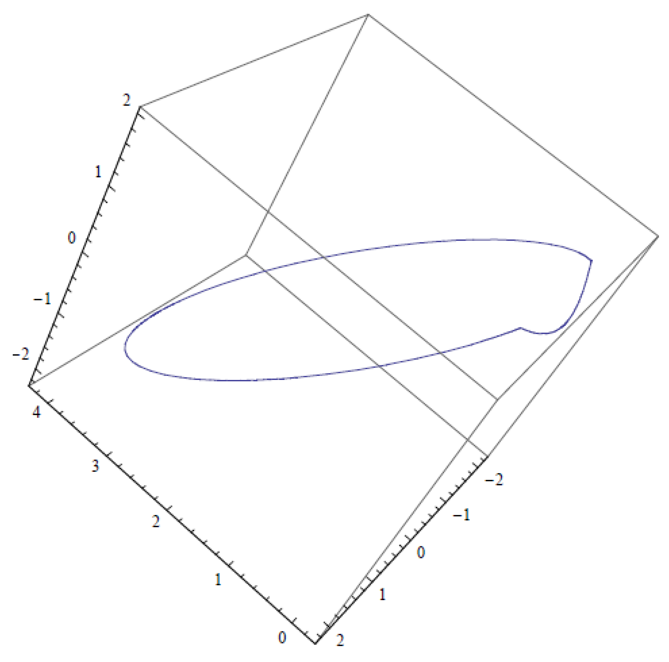
2.4. Periodic Orbits of a Relay System in ${\mathbb{R}}^3$

Consider the discontinuous piecewise linear differential system:

$$\dot{x}=y,\dot{y}=z,\dot{z}=-\mathrm{sign}\left(x\right)y.$$

(19)

Then, the goal of this subsection was to analytically study the periodic orbits of this differential system using their first integrals. The sign function is given by:

$$\mathrm{sign}\left(x\right)=\left\{\begin{array}{cc}-1& \mathrm{if} x<0,\hfill \\ 0& \mathrm{if} x=0,\hfill \\ 1& \mathrm{if} x>0.\hfill \end{array}\right.$$

Therefore, $x=0$ is the plane of discontinuity of system (19). System (19) was studied in [27].

Many discontinuous piecewise differential systems (19) appear in a natural way from the control theory. In fact, system (19) is a particular relay system of the ones studied in [28].

In general, a difficult problem is to analytically find the periodic solutions of a differential system; usually, this problem cannot be solved. We wanted to compute the periodic orbits of continuous or discontinuous piecewise differential systems such that they are completely integrable in each piece.

The objective of this subsection was to prove the next result.

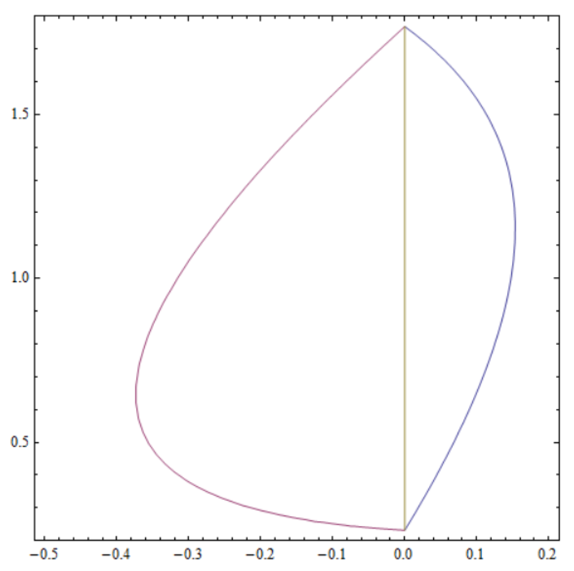
Theorem 4.

The following statements hold:

(a) 

Assume that the discontinuous piecewise linear differential system (19) has a periodic orbit γ such that intersects $x=0$ in two points. Then, these two points are $(0,y,z)$ and $(0,-y,z)$ with $z>0$ and $y^2-z^2<0$. See Figure 4.

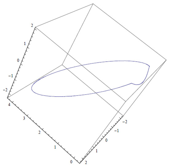Figure 4. The periodic orbit of Theorem 4 intersecting $x=0$ in the points $(0,-1,2)$ and $(0,1,2)$.

(b) 

For every pair of points $(0,y,z)$ and $(0,-y,z)$ with $z>0$ and $y^2-z^2<0$, the discontinuous piecewise linear differential system (19) has a periodic orbit γ intersecting $x=0$ in these two points.

Proof. 

The discontinuous piecewise linear differential system (19) in $x>0$ is given by:

$$\dot{x}=y,\dot{y}=z,\dot{z}=-y,$$

(20)

and in $x<0$ by:

$$\dot{x}=y,\dot{y}=z,\dot{z}=y.$$

(21)

Observe that the points of the x–axis are equilibrium points.

We could obtain two independent first integrals for the systems (20) and (21) because these differential systems are linear. Linear differential systems are completely Darboux integrable; for more details, see [24]. Therefore, for system’s (20) two independent first integrals are:

$$H_1=x+z,\mathrm{and}{H}_2=y^2+z^2.$$

Hence, the trajectories of system (20) are contained in:

$${\gamma }_{h_1{h}_2}=\{H_1=h_1\}\cap \{H_2=h_2\}\cap \{x>0\},$$

for all $(h_1,h_2)\in {\mathbb{R}}^2$.

For system (21), the two independent first integrals are

$$F_1=x-z,\mathrm{and}{F}_2=y^2-z^2.$$

Hence, the trajectories of system (21) are contained in:

$${\gamma }_{f_1{f}_2}=\{F_1=f_1\}\cap \{F_2=f_2\}\cap \{x<0\},$$

for all $(f_1,f_2)\in {\mathbb{R}}^2$.

The set ${\gamma }_{h_1{h}_2}$ with $h_2>0$ is composed in $x>0$ by the intersection of the plane $H_1=h_1$ with the cylinder $H_2=h_2$. Therefore, the set ${\gamma }_{h_1{h}_2}$ is an arc without equilibria, and it is a trajectory of system (20). If $h_2=0$, then ${\gamma }_{h_1{h}_2}$ is an equilibrium point. Hence, ${\gamma }_{h_1{h}_2}$ is a unique orbit of system (20).

If $f_2\ne 0$, the set ${\gamma }_{f_1{f}_2}$ in $x<0$ is one or two arcs of the intersection of the plane $F_1=f_1$ with the hyperboloid cylinder $F_2=f_2$, these arcs have no equilibria. Therefore, ${\gamma }_{f_1{f}_2}$ has one or two trayectories of system (21). If $f_2=0$, then ${\gamma }_{f_1{f}_2}$ in $x<0$ is the intersection of the plane $F_1=f_1$ with the two planes $F_2=0$. The intersection $\{F_1=f_1\}\cap \{F_2=0\}$ in $x<0$ is two straight lines which intersect at the equilibrium point $(f_1,0,0)$. Such intersections are formed by 5 or 2 trajectories, respectively.

We analyzed when a trajectory of ${\gamma }_{h_1{h}_2}$ and a trajectory of ${\gamma }_{f_1{f}_2}$ gave place to a periodic orbit of the system (19). From above, if $h_2>0$ and $f_2\ne 0$, then the trajectories of systems (20) and (21) could connect, forming a periodic orbit.

In the plane of discontinuity $x=0$, we considered the point $(0,y_0,z_0)$. Let $h_1=z_0$, $h_2=y_0^2+z_0^2$, $f_1=-z_0$ and $f_2=y_0^2-z_0^2$ be the four values of the first integrals $H_1$, $H_2$, $F_1$, and $F_2$ at this point, respectively. Now, we studied the points of the trajectory $\{H_1=h_1\}\cap \{H_2=h_2\}\cap \{x\ge 0\}$ contained in $x=0$. This was conducted by solving the system:

$$H_1=h_1,H_2=h_2,x=0.$$

This system provides the two points $(0,\pm y_0,z_0)$. The points of the trajectory $\{F_1=f_1\}\cap \{F_2=f_2\}\cap \{x\le 0\}$ in $x=0$, are studied solving the system

$$F_1=f_1,F_2=f_2,x=0.$$

This system provides the two points $(0,\pm y_0,z_0)$. When these pair of points are in the same trajectory $\{F_1=f_1\}\cap \{F_2=f_2\}\cap \{x\le 0\}$, we obtained a periodic orbit of the system (19).

In $x\ge 0$, using the variable x, we parameterized the trajectory $\{H_1=h_1\}\cap \{H_2=h_2\}$, obtaining the arc:

$$\{(x,\pm \sqrt{y_0^2+z_0^2-{(z_0-x)}^2},z_0-x):0\le x\le z_0+\sqrt{y_0^2+z_0^2}\}.$$

(22)

This trajectory in $x\ge 0$ is symmetric with respect to the y–axis with endpoints $(0,\pm y_0,z_0)$ in $x=0$.

In $x\le 0$, using the variable x, we parameterized the curve $\{F_1=f_1\}\cap \{F_2=f_2\}$, which is formed by the two trajectories:

• $\{(x,\pm \sqrt{x^2+y_0^2},x):x\le 0\}$ if $z_0=0$, each trajectory has one endpoint in $x=0$;
• $\{x,\pm \sqrt{{(x+z_0)}^2+y_0^2-z_0^2},z_0+x)\}:x\le 0\}$ if either $z_0<0$ or $z_0>0$ and $y_0^2-z_0^2>0$, each trajectory has one endpoint in $x=0$;
• $$\{x,\pm \sqrt{{(x+z_0)}^2+y_0^2-z_0^2},z_0+x)\}:-z_0+\sqrt{z_0^2-y_0^2}\le x\le 0\}$$

  (23)

  and

  $$\{x,\pm \sqrt{{(x+z_0)}^2+y_0^2-z_0^2},z_0+x)\}:x\le -z_0-\sqrt{z_0^2-y_0^2}\},$$

  if $z_0>0$ and $y_0^2-z_0^2<0$, the first trajectory has its two endpoints at the points $(0,\pm y_0,z_0)$ in $x=0$, and the second trajectory has its endpoints at infinity.

We note that $y_0^2-z_0^2\ne 0$; otherwise, $f_2=0$.

Summarizing, if $z_0>0$ and $y_0^2-z_0^2<0$, the trajectory (22) of system (20) with the trajectory (23) of system (21) provides a periodic orbit of system (19), and this periodic orbit intersects $x=0$ in the points $(0,\pm y_0,z_0)$. Hence, Theorem 4 was proved. □

2.5. Limit Cycles of a Class of Piecewise Differential Systems Separated by a Parabola

The goal of this subsection was to analyze the limit cycles of discontinuous piecewise differential systems separated by the parabola $y=x^2$ and formed by two linear Hamiltonian systems without equilibrium points.

Easy computations show that a linear Hamiltonian system without equilibrium points must be of the form:

$$X_i(x,y)=(-{\lambda }_i{b}_{i}x+b_{i}y+{\gamma }_i,-{\lambda }_i^2{b}_{i}x+{\lambda }_i{b}_{i}y+{\delta }_i),$$

${\delta }_i\ne {\lambda }_i{\gamma }_i$ and $b_i\ne 0$, with $i=1\cdots 4$, and its corresponding Hamiltonian function is:

$$H_i(x,y)=(-{\lambda }_i^2{b}_i/2)x^2+{\lambda }_i{b}_{i}xy-(b_i/2)y^2+{\delta }_{i}x-{\gamma }_{i}y.$$

We wanted to prove the following result, which came from [29].

Theorem 5.

Generically, the maximum number of limit cycles of the piecewise differential systems separated by the parabola $y=x^2$ and formed by two linear Hamiltonian systems without equilibrium points is two, and this maximum is reached, see Figure 5.

Figure 5. Two limit cycles of a piecewise differential system separated by the parabola $y=x^2$ and formed by two linear Hamiltonian systems without equilibrium points. Both limit cycles travel in counterclockwise sense.

Proof. 

In region $R_1=\{(x,y):y-x^2\ge 0\}$, we considered the linear Hamiltonian system without equilibrium points:

$$\dot{x}=-{\lambda }_1{b}_{1}x+b_{1}y+{\gamma }_1,\dot{y}=-{\lambda }_1^2{b}_{1}x+{\lambda }_1{b}_{1}y+{\delta }_1,$$

(24)

with $b_1\ne 0$ and ${\delta }_1\ne {\lambda }_1{\gamma }_1$. Its corresponding Hamiltonian function is:

$$H_1(x,y)=-({\lambda }_1^2{b}_1/2)x^2+{\lambda }_1{b}_{1}xy-(b_1/2)y^2+{\delta }_{1}x-{\gamma }_{1}y.$$

(25)

In region $R_2=\{(x,y):y-x^2\le 0\}$, we considered another linear Hamiltonian system without equilibrium points:

$$\dot{x}=-{\lambda }_2{b}_{2}x+b_{2}y+{\gamma }_2,\dot{y}=-{\lambda }_2^2{b}_{2}x+{\lambda }_2{b}_{2}y+{\delta }_2,$$

(26)

with $b_2\ne 0$ and ${\delta }_2\ne {\lambda }_2{\gamma }_2$. Its corresponding Hamiltonian function is:

$$H_2(x,y)=-({\lambda }_2^2{b}_2/2)x^2+{\lambda }_2{b}_{2}xy-(b_2/2)y^2+{\delta }_{2}x-{\gamma }_{2}y.$$

(27)

In order to have a crossing limit cycle which intersects the parabola $y-x^2=0$ in the points $(x_i,x_i^2)$ and $(x_k,x_k^2)$, these points must satisfy the following system:

$$\begin{array}{c}{H}_1(x_i,x_i^2)-H_1(x_k,x_k^2)=0,\hfill \\ H_2(x_i,x_i^2)-H_2(x_k,x_k^2)=0,\hfill \end{array}$$

(28)

We supposed that the two systems (24) and (26) have three crossing limit cycles, and we arrived to a contradiction. Then, system (28) must have three pairs of points as solutions, namely, $p_i=(r_i,r_i^2)$ and $q_i=(s_i,s_i^2)$, with $i=1,2,3$.

Since the points $p_1=(r_1,r_1^2)$ and $q_1=(s_1,s_1^2)$ satisfy system (28), we obtained that the parameters ${\gamma }_1$ and ${\gamma }_2$ must be:

$$\begin{array}{cc}\hfill {\gamma }_1=& {\displaystyle \frac{1}{2(r_1+s_1)}}(-r_1{r}_1^3-b_1{r}_1^2{s}_1-b_1{r}_1{s}_1^2-b_1{s}_1^3+2{\delta }_1+2b_1{r}_1^2{\lambda }_1+2b_1{r}_1{s}_1{\lambda }_1\hfill \\ & +2b_1{s}_1^2{\lambda }_1-b_1{r}_1{\lambda }_1^2-b_1{s}_1{\lambda }_1^2),\hfill \end{array}$$

and ${\gamma }_2$ has the same expression that ${\gamma }_1$ changes $(b_1,{\lambda }_1,{\delta }_1)$ by $(b_2,{\lambda }_2,{\delta }_2)$.

If the second points $p_2=(r_2,r_2^2)$ and $q_2=(s_2,s_2^2)$ satisfy system (28), then the parameters ${\delta }_1$ and ${\delta }_2$ must be:

$$\begin{array}{cc}\hfill {\delta }_1=& {\displaystyle \frac{b_1}{2(r_1-r_2+s_1-s_2)}}(-r_1^3{r}_2-r_1{r}_2^3+r_1^2{r}_2{s}_1-r_2^3{s}_1+r_1{r}_2{s}_1^2+r_2{s}_1^3+r_1^3{s}_2\hfill \\ & -r_1{r}_2^2{s}_2+r_1^2{s}_1{s}_2-r_2^2{s}_1{s}_2+r_1{s}_1^2{s}_2+s_1^3{s}_2-r_1{r}_2{s}_2^2-r_2{s}_1{s}_2^2-r_1{s}_2^3-s_1{s}_2^3\hfill \\ & -2r_1^2{r}_2{\lambda }_1+2r_1{r}_2^2{\lambda }_1-2r_1{r}_2{s}_1{\lambda }_1+2r_2^2{s}_1{\lambda }_1-2r_2{s}_1^2{\lambda }_1-2r_1^2{s}_2{\lambda }_1+2r_1{r}_2{s}_2{\lambda }_1\hfill \\ & -2r_1{s}_1{s}_2{\lambda }_1+2r_2{s}_1{s}_2{\lambda }_1-2s_1^2{s}_2{\lambda }_1+2r_1{s}_2^2{\lambda }_1+2s_1{s}_2^2{\lambda }_1),\hfill \end{array}$$

and ${\delta }_2$ has the same expression that ${\delta }_1$ changes $(b_1,{\lambda }_1)$ by $(b_2,{\lambda }_2)$.

Finally, we supposed that the points $p_3=(r_3,r_3^2)$ and $q_3=(s_3,s_3^2)$ satisfy system (28); then, the parameters ${\lambda }_1$ and ${\lambda }_2$ must be ${\lambda }_1=A/B$, where:

$$\begin{array}{cc}\hfill A=& r_1^3(r_2-r_3+s_2-s_3)+r_1^2{s}_1(r_2-r_3+s_2-s_3)+r_2^3(r_3-s_1+s_3)+r_2^2{s}_2(r_3-s_1\hfill \\ & +s_3)+r_1(-r_2^3+r_3^3-r_3{s}_1^2-r_2^2{s}_2+s_1^2{s}_2-s_2^3+r_2(s_1^2-s_2^2)+r_3^2{s}_3-s_1^2{s}_3+r_3{s}_3^2\hfill \\ & +s_3^3)+(s_1-s_2)(r_3^3+r_3^2{s}_3+(s_1-s_3)(s_2-s_3)(s_1+s_2+s_3)-r_3(s_1^2+s_1{s}_2+s_2^2\hfill \\ & -s_3^2\left)\right)-r_2(r_3^3-s_1^3+s_1{s}_2^2+r_3^2{s}_3-s_2^2{s}_3+s_3^3+r_3(-s_2^2+s_3^2)),\hfill \\ \hfill B=& 2((s_1-s_2)(r_3^2+(s_1-s_3)(s_2-s_3)-r_3(s_1+s_2-s_3))+r_1^2(r_2-r_3+s_2-s_3)\hfill \\ & +r_2^2(r_3-s_1+s_3)+r_1(-r_2^2+r_3^2-r_3{s}_1+r_2(s_1-s_2)+s_1{s}_2-s_2^2+r_3{s}_3-s_1{s}_3\hfill \\ & +s_3^2)-r_2(r_3^2+r_3(-s_2+s_3)-(s_1-s_3)(s_1-s_2+s_3)).\hfill \end{array}$$

Furthermore, ${\lambda }_2$ has the same expression that ${\lambda }_1$ changes $b_1$ by $b_2$.

We replaced ${\gamma }_1$, ${\lambda }_1$ and ${\delta }_1$ in the expression of $H_1(x,y)$, and ${\gamma }_2$, ${\lambda }_2$ and ${\delta }_2$ in the expression of $H_2(x,y)$, and we obtained $H_1(x,y)=H_2(x,y)$. Therefore, the two linear differential systems forming the piecewise system coincide. Therefore the piecewise system has no limit cycles. Consequently, two is the maximum number of limit cycles.

To complete the proof of the theorem, we presented a discontinuous piecewise differential system satisfying the assumptions of the theorem, having two limit cycles.

Let the parabola $y=x^2$ be the discontinuity line of the piecewise differential system formed by the following two linear Hamiltonian systems without equilibria:

$$\dot{x}=5.5x-0.5y+3,\dot{y}=60.5x-5.5y+0.2,$$

(29)

in the region $R_1$ its Hamiltonian is:

$$H_1(x,y)=30.25x^2-5.5xy+0.2x+0.25y^2-3y.$$

The second system is:

$$\dot{x}=0.2x-0.1y-0.778814,\dot{y}=0.4x-0.2y+0.00727332,$$

(30)

in the region $R_2$, its Hamiltonian is:

$$H_2(x,y)=0.2x^2-0.2xy+0.00727332x+0.05y^2+0.778814y.$$

This piecewise differential system has the limit cycles shown in Figure 5. Therefore, Theorem 5 was proved. □

2.6. Piecewise Differential System with a Non-Regular Discontinuity Line

The extended 16th Hilbert problem consists of finding, for a given class of differential systems, an upper bound for the maximum number of their limit cycles. This is, in general, a very difficult problem, in general unsolved.

Only for very few classes of differential systems this problem has been solved.

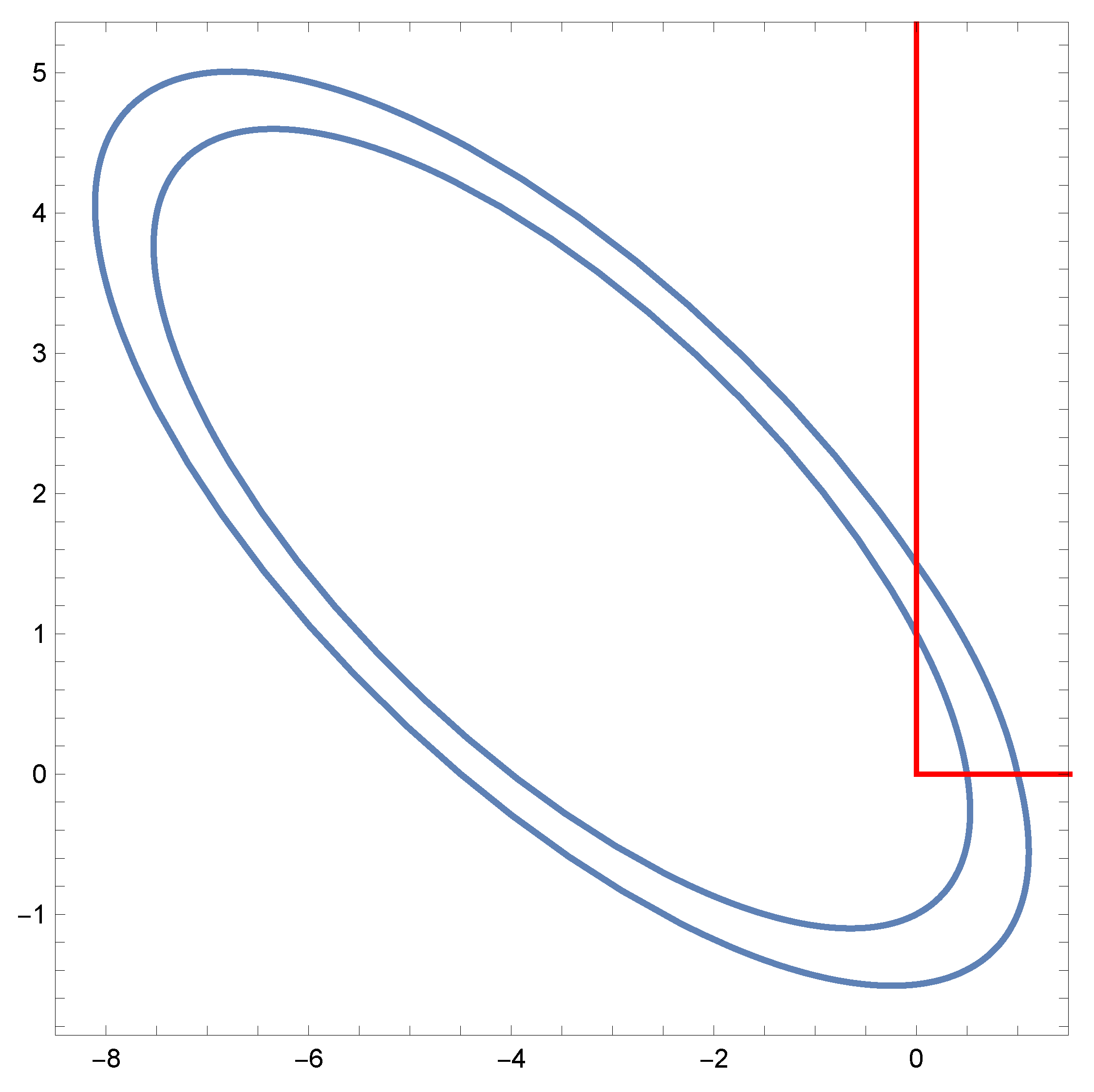
Now, we studied the extended 16th Hilbert problem for the piecewise differential systems separated by the non-regular line $\mathcal{R}$ formed by the two positive half-axes x and y, and formed by two linear centers.

We denoted by ${\mathcal{R}}_1$ the open positive quadrant of ${\mathbb{R}}^2$, and by ${\mathcal{R}}_2$ the interior of ${\mathbb{R}}^2\backslash {\mathcal{R}}_1$.

It is known that an arbitrary linear center can be written as:

$$\begin{array}{c}\dot{x}=-Ax-(A^2+{\Omega }^2)y+B,\hfill \\ \dot{y}=x+Ay+C,\hfill \end{array}\mathrm{for}(x,y)\in {\mathcal{R}}_1,$$

(31)

and

$$\begin{array}{c}\dot{x}=-ax-(a^2+{\omega }^2)y+b,\hfill \\ \dot{y}=x+ay+c,\hfill \end{array}\mathrm{for}(x,y)\in {\mathcal{R}}_2,$$

(32)

with $\Omega ,\omega >0$, $A,B,C,a,b,c\in \mathbb{R}$, and $A,a\ne 0$.

Each system (31) and (32) have, respectively, the first integrals:

$$\begin{array}{cc}\hfill H_1(x,y)& ={(x+Ay)}^2+2(Cx-By)+y^2{\Omega }^2,\hfill \\ \hfill H_2(x,y)& ={(x+ay)}^2+2(cx-by)+y^2{\omega }^2.\hfill \end{array}$$

(33)

The next result appears in [30].

Theorem 6.

Consider the two arbitrary linear differential centers (31) and (32) forming the discontinuous piecewise differential systems separated by the non-regular line $\mathcal{R}$. Then, the maximum number of limit cycles of these piecewise systems intersecting $\mathcal{R}$ in two points is two. Moreover there exist systems with exactly two limit cycles of this type, see Figure 6.

Figure 6. Both limit cycles are travelled in counter-clockwise sense.

Proof. 

We considered the discontinuous planar linear differential systems (31) and (32). If there exists a crossing limit cycle intersecting the non-regular separation curve $\mathcal{R}$, in two points of the forms $(x,0)$ and $(0,y)$ both are different from the origin. Since the functions $H_1$ and $H_2$ defined in (33) are first integrals of the systems (31) and (32), respectively, these points must satisfy the equations:

$$\begin{array}{cc}\hfill e_1:=H_1(x,0)-H_1(0,y)& =2Cx+x^2+2By-A^2{y}^2-y^2{\Omega }^2=0,\hfill \\ \hfill e_2:=H_2(x,0)-H_2(0,y)& =2cx+x^2+2by-a^2{y}^2-y^2{\omega }^2=0.\hfill \end{array}$$

(34)

By using the Bézout theorem, this system can have, at most, four isolated solutions, one of them being the origin.

In order to obtain crossing limit cycles, equations $e_1=0$ and $e_2=0$ must have isolated solutions $(x_i,y_i)$ with $x_i,y_i>0$. Therefore, there are at most three crossing limit cycles of system $e_1=e_2=0$. In order for these three solutions $(x_i,y_i)$ to produce limit cycles, it is necessary that:

$$0<x_1<x_2<x_3\mathrm{and}0<y_1<y_2<y_3.$$

We claimed that there are at most two solutions $(x_1,y_1)$ and $(x_2,y_2)$ providing limit cycles, that is, satisfying:

$$0<x_1<x_2\mathrm{and}0<y_1<y_2.$$

(35)

Now, we proved the claim.

If $a^2+{\omega }^2-A^2-{\Omega }^2=0$, then the piecewise system has at most one limit cycle. Indeed, the resultant of the polynomial $e_1$ and $e_2$ with respect to the variable y is:

$$\begin{array}{c}4x\left(a^2+{\omega }^2\right)(x\left(a^2{c}^2-2a^{2}cC+a^2{C}^2-b^2+2bB-B^2+c^2{\omega }^2-2cC{\omega }^2+C^2{\omega }^2\right)\hfill \\ -2(b-B)(bC-Bc)).\hfill \end{array}$$

Therefore, at most, one positive solution of x, consequently, is at most one limit cycle.

Assume now that $a^2+{\omega }^2-A^2-{\Omega }^2\ne 0$.

Equations $e_1=e_2=0$ are equivalent to equations $E_1=e_1-e_2=0$ and $E_2=e_1(a^2+{\omega }^2)-e_2(A^2+{\Omega }^2)=0$, i.e.,:

$$\begin{array}{cc}\hfill E_1=& 2(C-c)x+2(B-b)y-(A^2+{\Omega }^2-a^2-{\omega }^2))y^2=0,\hfill \\ \hfill E_2=& 2\left((a^2+{\omega }^2)C-(A^2+{\Omega }^2)c\right)x+2\left((a^2+{\omega }^2)B-(A^2+{\Omega }^2)b\right)y\hfill \\ \hfill & +(a^2+{\omega }^2-A^2-{\Omega }^2)x^2=0.\hfill \end{array}$$

(36)

If $C=c$, then $E_1=0$ reduces to either one horizontal straight line, or two horizontal parallel straight lines passing one of these two straight lines through the origin. The equation $E_2=0$ is either a parabola symmetric with respect to some vertical straight line, one vertical straight line, or two vertical parallel straight lines passing one of these two straight lines through the origin. Since $E_1=E_2=0$ pass through the origin, there are at most two intersection points satisfying (35) and so, at most, two limit cycles.

Assume now that $C\ne c$. In this case, $E_1=0$ is a parabola symmetric with respect to some horizontal straight line and $E_2=0$ is a parabola symmetric with respect to some vertical straight line. Since both parabolas intersect at the origin, there are at most two intersection points satisfying (35), and so, at most, two limit cycles. This proves the claim and, consequently, the theorem once we provided an example with two limit cycles.

Now, we gave a discontinuous piecewise linear differential system (31)–(32) having exactly two limit cycles intersecting in two points the discontinuity line $\mathcal{R}$. In region ${\mathcal{R}}_1$, we considered the linear differential center:

$$\dot{x}=-2x-8y-{\displaystyle \frac{3}{2}},\dot{y}=x+2y+{\displaystyle \frac{43}{4}},$$

(37)

with the first integral:

$$H_1(x,y)=4y^2+2\left({\displaystyle \frac{43}{4}}x+{\displaystyle \frac{3}{2}}y\right)+{(x+2y)}^2;$$

and in region ${\mathcal{R}}_2$, we considered the linear differential center:

$$\dot{x}=-x-2y,\dot{y}=x+y+{\displaystyle \frac{7}{4}},$$

(38)

with the first integral:

$$H_2(x,y)=y^2+{\displaystyle \frac{7}{2}}x+{(x+y)}^2.$$

In this case, the two solutions of Equation (36) are:

$$(x_1,y_1)=\left({\displaystyle \frac{1}{2}},1\right),(x_2,y_2)=\left(1,{\displaystyle \frac{3}{2}}\right),$$

and the corresponding limit cycles are shown in Figure 2. □

3. Discussion

In this paper, we summarized the main results on the Darboux theory of integrability for finding first integrals. We illustrated, with some relevant examples, the different main ingredients of this theory, as the invariant algebraic curves, the exponential factors, the integrating factors, and the first integrals.

After, we used the first integrals of distinct classes of piecewise differential systems for studying the limit cycles of these differential systems in ${\mathbb{R}}^2$ and ${\mathbb{R}}^3$. Thus, first we studied the limit cycles of a discontinuous piecewise differential system in ${\mathbb{R}}^2$ with two zones separated by a straight line and formed by a linear differential center and a quadratic polynomial differential system.

After, we computed the three limit cycles of a piecewise differential system in ${\mathbb{R}}^2$ with three zones separated by the non-regular line:

$$\{(x,y)\in {\mathbb{R}}^2:y=0\mathrm{or}x=0\mathrm{and}y\ge 0\},$$

and each zone having an arbitrary linear differential system.

We also studied the periodic orbits of a relay system in ${\mathbb{R}}^3$.

We analyzed the limit cycles of discontinuous piecewise differential systems in ${\mathbb{R}}^2$ with two zones separated by a parabola and each zone having a Hamiltonian system without equilibrium points.

Finally, we proved that the maximum number of limit cycles of a piecewise differential system in ${\mathbb{R}}^2$ with two zones separated by the non-regular line formed by the positive x and y half-axes and having, in each zone, an arbitrary linear differential system was two. We also provided an example of these differential systems having exactly two limit cycles.

4. Conclusions

We illustrated how to compute first integrals of the polynomial differential systems via the Darboux theory of integrability, and we also illustrated how to compute periodic orbits and limit cycles of different classes of piecewise differential systems using their first integrals.

References

- Whittaker, E.T. A Treatise on the Analytical Dynamics of Particles and Rigid Bodies; Cambridge Mathematical Library, Cambridge University Press: Cambridge, UK, 1988. [Google Scholar]
- Dumortier, F.; Llibre, J.; Artés, J.C. Qualitative Theory of Planar Differential Systems; UniversiText; Springer: New York, NY, USA, 2006. [Google Scholar]
- Olver, P.J. Applications of Lie Groups to Differential Equations, 2nd ed.; Graduate Texts in Mathematics; Springer: New York, NY, USA, 1993; Volume 107. [Google Scholar]
- di Bernardo, M.; Budd, C.J.; Champneys, A.R.; Kowalczyk, P. Piecewise-Smooth Dynamical Systems: Theory and Applications; Applied Mathematical Sciences; Springer: London, UK, 2008; Volume 163. [Google Scholar]
- Leine, R.I.; Nijmeijer, H. Dynamics and Bifurcations of Non-Smooth Mechanical Systems; Lecture Notes in Applied and Computational Mechanics; Springer: Berlin/Heidelberg, Germany, 2004; Volume 18. [Google Scholar]
- Liberzon, D. Switching in Systems and Control: Foundations and Applications; Birkhäuse: Boston, MA, USA, 2003. [Google Scholar]
- Simpson, D.J.W. Bifurcations in Piecewise-Smooth Continuous Systems; World Scientific Series on Nonlinear Science Series A; World Scientific: Singapore, 2010; Volume 69. [Google Scholar]
- Makarenkov, O.; Lamb, J.S.W. Dynamics and bifurcations of nonsmooth systems: A survey. Physica D 2012, 241, 1826–1844. [Google Scholar] [CrossRef] [Green Version]
- Filippov, A.F. Differential Equations with Discontinuous Right-Hand Sides; Kluwer Academic: Dordrecht, The Netherlands, 1988. [Google Scholar]
- Lum, R.; Chua, L.O. Global propierties of continuous piecewise-linear vector fields. Part I: Simplest case in ℝ2. Int. J. Circuit Theory Appl. 1991, 19, 251–307. [Google Scholar] [CrossRef]
- Huan, S.M.; Yang, X.S. Existence of limit cycles in general planar piecewise linear systems of saddle–saddle dynamics. Nonlinear Anal. 2013, 92, 82–95. [Google Scholar] [CrossRef]
- Braga, D.C.; Mello, L.F. Limit cycles in a family of discontinuous piecewise linear differential systems with two zones in the plane. Nonlinear Dynam. 2013, 73, 1283–1288. [Google Scholar] [CrossRef]
- Buzzi, C.; Gasull, A.; Torregrosa, J. Algebraic limit cycles in piecewise linear differential systems. Int. J. Bifurc. Chaos 2018, 28, 1850039. [Google Scholar] [CrossRef]
- Buzzi, C.; Pessoa, C.; Torregrosa, J. Piecewise linear perturbations of a linear center. Discret. Contin. Dyn. Syst. 2013, 33, 3915–3936. [Google Scholar] [CrossRef] [Green Version]
- Freire, E.; Ponce, E.; Rodrigo, F.; Torres, F. Bifurcation sets of continuous piecewise linear systems with two zones. Int. J. Bifurc. Chaos 1998, 8, 2073–2097. [Google Scholar] [CrossRef]
- Freire, E.; Ponce, E.; Torres, F. Canonical Discontinuous Planar Piecewise Linear Systems. SIAM J. Appl. Dyn. Syst. 2012, 11, 181–211. [Google Scholar] [CrossRef]
- Freire, E.; Ponce, E.; Torres, F. A general mechanism to generate three limit cycles in planar Filippov systems with two zones. Nonlinear Dyn. 2014, 78, 251–263. [Google Scholar] [CrossRef]
- Giannakopoulos, F.; Pliete, K. Planar systems of piecewise linear differential equations with a line of discontinuity. Nonlinearity 2001, 14, 1611–1632. [Google Scholar] [CrossRef]
- Han, M.; Zhang, W. On Hopf bifurcation in non—Smooth planar systems. J. Differ. Equ. 2010, 248, 2399–2416. [Google Scholar] [CrossRef] [Green Version]
- Huan, S.M.; Yang, X.S. On the number of limit cycles in general planar piecewise systems. Discret. Cont. Dyn. Syst. Ser. A 2012, 32, 2147–2164. [Google Scholar] [CrossRef]
- Li, L. Three crossing limit cycles in planar piecewise linear systems with saddle-focus type. Electron. J. Qual. Theory Differ. Equ. 2014, 70, 1–14. [Google Scholar] [CrossRef]
- Wang, J.; Huang, C.; Huang, L. Discontinuity-induced limit cycles in a general planar piecewise linear system of saddle-focus type. Nonlinear Anal. Hybrid Syst. 2019, 33, 162–178. [Google Scholar] [CrossRef]
- Chen, H.; Li, D.; Xie, J.; Yue, Y. Limit cycles in planar continuous piecewise linear systems. Commun. Nonlinear Sci. Numer. Simul. 2017, 47, 438–454. [Google Scholar] [CrossRef]
- Falconi, M.; Llibre, J. n − 1 independent first integrals for Linear differential systems in ℝn and ℂn. Qual. Theory Dyn. Syst. 2004, 4, 233–254. [Google Scholar] [CrossRef]
- Schlomiuk, D. Algebraic particular integrals, integrability and the problem of the center. Trans. Am. Math. Soc. 1993, 338, 799–841. [Google Scholar] [CrossRef]
- Llibre, J.; Zhang, X. Limit cycles created by piecewise linear centers. Chaos 2019, 29, 053116. [Google Scholar] [CrossRef] [PubMed]
- Llibre, J.; Teixeira, M.A. Periodic orbits of continuous and discontinuous piecewise linear differential systems via first integrals. Sao Paulo J. Math. Sci. 2018, 12, 121–135. [Google Scholar] [CrossRef] [Green Version]
- Anosov, D.V. Stability of the equilibrium positions in relay systems. Avtomatika i Telemehanika 1959, 20, 135–149. [Google Scholar]
- Benterki, R.; Llibre, J. Crossing Limit cycles of planar piecewise linear Hamiltonian systems without equilibrium points. Mathematics 2020, 8, 755. [Google Scholar] [CrossRef]
- Esteban, M.; Llibre, J.; Valls, C. The extended 16-th Hilbert problem for discontinuous piecewise isochronous centers of degree one or two separated by a straight line. Int. J. Bifurc. Chaos 2021, 31, 043112. [Google Scholar] [CrossRef]
Publisher’s Note: MDPI stays neutral with regard to jurisdictional claims in published maps and institutional affiliations. |
© 2021 by the author. Licensee MDPI, Basel, Switzerland. This article is an open access article distributed under the terms and conditions of the Creative Commons Attribution (CC BY) license (https://creativecommons.org/licenses/by/4.0/).