Abstract
In this paper, the Singular-Polynomial-Fuzzy-Model (SPFM) approach problem and impulse elimination are investigated based on sliding mode control for a class of nonlinear singular system (NSS) with impulses. Considering two numerical examples, the SPFM of the nonlinear singular system is calculated based on the compound function type and simple function type. According to the solvability and the steps of two numerical examples, the method of solving the SPFM form of the nonlinear singular system with (and without) impulse are extended to the more general case. By using the Heine–Borel finite covering theorem, it is proven that a class of nonlinear singular systems with bounded impulse-free item (BIFI) properties and separable impulse item (SII) properties can be approximated by SPFM with arbitrary accuracy. The linear switching function and sliding mode control law are designed to be applied to the impulse elimination of SPFM. Compared with some published works, a human posture inverted pendulum model example and Example 3.2 demonstrate that the approximation error is small enough and that both algorithms are effective. Example 3.3 is to illustrate that sliding mode control can effectively eliminate impulses of SPFM.
1. Introduction
The Takagi–Sugeno (T-S) fuzzy model was put forward by T. Takagi and M. Sugeno [1] in 1985, and they proposed a new type of fuzzy model representation. Due to the excellent approximation performance of the T-S fuzzy model in nonlinear systems, more and more scholars are interested in the T-S fuzzy model using multiple local linear systems to represent the nonlinear system and then analyzing the characteristics of the nonlinear system by using the analysis method of the linear system. In 1992, an important conclusion was proved by Wang [2], that is, fuzzy systems are a universal approximator, and Wang approximated any continuous function on the compact set with any precision by using the fuzzy system constructed with gaussian membership functions, a product inference machine, and a center-average weighted defuzzifer. Since then, many scholars [3,4,5,6,7] have proven that the above conclusions can be adapted to various fuzzy systems. In [8], the finite-time stabilization of a class of stochastic nonlinear systems was studied by applying the fuzzy-logic systems to approximate the unknown nonlinearities and a novel adaptive finite-time control strategy was proposed. The vector integral sliding mode surface and sliding mode control (SMC) law were proposed for the T-S fuzzy singular system with matched external disturbances in [9]. In recent years, a new fuzzy model has been proposed by K. Tanaka [10], that is, a polynomial fuzzy model. In essence, it is a more extensive form of the T-S fuzzy model. The main difference between the two models is the conclusion: the result of T-S fuzzy model is a linear model, and the result of polynomial fuzzy model is a polynomial model. Therefore, the number of fuzzy rules in the polynomial fuzzy model is much less than that in the T-S fuzzy model when describing the same nonlinear systems. Hence, it will become more and more popular, and more and more people [11,12,13] have begun to study the polynomial fuzzy system. In [14,15], the polynomial fuzzy singular system was proposed first and the interval observers for polynomial fuzzy singular systems were designed, in which the external disturbances and unknown parameters were included in the systems. However, Pang [14,15] assumed that the polynomial fuzzy singular systems is regular and impulse-free. In this paper, the SPFM can be obtained for the NSSs with the impulse by the SPFM approximation theorem and related algorithms given.
As the fuzzy modeling develops, polynomial fuzzy models employ polynomial models as local subsystems instead of linear models. It not only makes the modeling process simpler but also handles more nonlinear plant in comparison with the singular T-S fuzzy model. The LMI-based stability analysis method commonly used in T-S fuzzy model has some difficulties in the application of polynomial fuzzy models. Thus far, it has not been directly used in the stability analysis of polynomial model systems. Based on the difficulty of analyzing polynomial fuzzy models, the sum-of-squares based (SOSB) approaches emerges and occupies an important position in the polynomial fuzzy model, which can effectively deal with stability analysis problems [10]. In [10], the SOSB stability analysis of a polynomial fuzzy model is proposed under a parallel, distributed compensation strategy; hence, the fuzzy controller designed has the same membership function and fuzzy rules as the polynomial fuzzy model. In [16], the stability of the polynomial-fuzzy-model-based (PFMB) control system was investigated by using the SOSB stability analysis method and by considering the number of fuzzy rules and the shape of premise fuzzy membership functions. In [17,18], the condition of system conservative stability was obtained based on the piecewise linear membership function and the polynomial approximation membership function.
The singular system is a natural representation of objective system. It can be used to describe further characteristics of the system and has been widely applied in large system theory, singular perturbed theory, circuit theory, and economic theory [19,20,21,22,23]. In 1999, Taniguchi et al. combined the T-S fuzzy system with the singular system and promoted it to propose the T-S fuzzy singular system [24]. In recent years, various novel control techniques have been applied to the fuzzy singular system [25,26,27,28,29,30]. In many practical models, most of the systems are nonlinear and the nonlinearity of many nonlinear systems can be transformed into polynomials. If the T-S fuzzy system is used to approximate the nonlinear system, there are two challenges, namely, the number of rules is too many and the approximation accuracy is insufficient. However, the birth of the SPFM approximation method can be able to solve such problems and to effectively reduce the number of fuzzy rules for the impulse-free nonlinear system. There are two main characteristics of SPFM: 1. The SPFM is a class of more complex system including dynamic and non-dynamic constraints. 2. The number of fuzzy rules of the SPFM for nonlinear system is less than the normal fuzzy model, and the results are more simple.
The T-S fuzzy singular system is used to approximate the NSS, but there may be two problems for complex NSS. One is too many rules for the T-S fuzzy singular system, and the other is that the approximation error is large. However, the SPFM is able to solve such problems, and the number of fuzzy rules can be reduced for the impulse-free NSS [14,15]. If the NSS has an impulse, there is no method to show that SPFM can effectively approach such systems. Reference [31] deals with the existence of solutions to singular second-order differential equations with impulse effects and with the Dirichlet boundary conditions. However, the requirements of the thesis are very strict, and there are many assumptions. In [32], Zhang and Yuan dealt with the existence and multiplicity of solutions for the nonlinear Dirichlet value problem with impulses by using the variational methods and critical points theory. In [33], Nieto introduced the concept of a weak solution for a damped linear equation with Dirichlet boundary conditions and impulses. The above three papers dealt with impulse problems for second-order differential equations and did not give the case of higher-order differential equations. In [34,35], this technical note discusses to what extent the high-order sliding mode control may serve as an alternative to the conventional sliding mode control. The definitions of sliding mode order, relative degree, chattering attenuation, filtering, and implementation complexity constitute the scope of that discussion. In [36], Utkin systematically introduced the development of the theory of sliding modes, the design of sliding mode controller, and the application of sliding mode control. In this paper, a theorem using the SPFM to approximate the nonlinear singular system with impulses was proven for any order and the assumptions were easier to satisfy. Our major research interest is to study the SPFM approach problem for a class of NSS with impulses. The main contributions of this paper are summarized below.
- (1)
- The method using SPFM to approximate the impulse-free nonlinear singular system is basically the same as the T-S fuzzy model, and there are many related studies. One of the important differences between singular systems and normal systems is that the former may contain impulse terms in the solution. Hence, the impulses are a distinctive feature of singular systems, and they are the basis on which singular systems can describe a wider range of physical systems. Current research on singular systems often ignores the impulses or assumes that the system is impulse-free and that there is no method to approximate the singular system with an impulse by using SPFM. The theorem that the SPFM can approximate an NSS with impulses with an arbitrary precision is proven.
- (2)
- According to the complexity of the NSS, it is divided into a nonlinear model with a compound function type and a simple function type. For two different types of NSS, two different theorems are given to prove the effectiveness of SPFM. It is fully proven that the NSS can be approximated using the SPFM model, even if the NSS has impulses. Then, the algorithms solving SPFM for two kinds of nonlinear functions are given.
- (3)
- The principle of SMC to eliminate the impulse is given. The designed SMC law not only can effectively eliminate impulses of SPFM but also can make the systems asymptotically stable.
The organizational structure of the paper is as follows. The descriptions of the approximation of SPFM are considered in Section 2. Two numerical examples of different types about NSSs and the corresponding algorithms for solving the SPEM for the NSS with (and without) impulses are given in Section 3. Then, the linear switching function and SMC law are designed, and two important theorems in SMC are proven. Finally, the theorem that the impulse of the SPFM can be eliminated by the SMC law is proven and the principle of SMC to eliminate the impulse is given. In Section 4, a human posture inverted pendulum model and two numerical example are presented to demonstrate the effectiveness of our theoretical results. Section 5 concludes the paper.
Notation: The symbol denotes the transposition of vector or matrix A; the symbol represents the n-dimensional vector space; represents Euclidean norm; represents supremum function; represents dimensional zero matrix; and the symbol ∗ represents entries.
2. Preliminaries and Problem Formulation
In this paper, we use the SPFM to approximate NSSs with (or without) impulses with any precision. Based on the sector nonlinearity concept, the singular polynomial fuzzy system can be represented.
Model Rules i:
where is the state vector, is the input vector, and is the fuzzy set of the rule i corresponding to the premise variable . is a matrix, , , and are the polynomial matrices about . The term is a monomial about , and each monomial is a function of form , where are integers, . Thus, is a polynomial vector.
As the fuzzy model develops, polynomial fuzzy models employ polynomial models as local subsystems, and polynomial fuzzy models is a more general case of T-S models. According to model rules and process of T-S model, the SPFM can be represented as
where
and
So
Remark 1.
The SPFM is the more extensive form of the T-S fuzzy singular system. If and are constant matrices ( and ) and , then becomes and it is the part of the T-S fuzzy singular system.
The SPFM approximation method has an important advantage that the number of fuzzy rules in a singular polynomial fuzzy system is generally fewer than the T-S fuzzy singular system.
Assumption 1.
In this paper, we assume that if and only if .
Remark 2.
Assumption 1 is mainly to ensure that the system is a polynomial about and that the constant term is 0. This is an important premise of polynomial systems, and many results have related assumptions [37].
The NSS is given as follows:
where is a n-dimensional vector function consisting of continuous function and .
Let P and Q be invertible matrices and . Let , where , the Equation (2) is equivalent to the following equation:
The research interest of this paper is to find the SPFM to approximate the NSS such as Equations (2) or (3).
Definition 1
(singularity induced bifurcations (SIB) [38]). Consider the system
Suppose that the system has an equilibrium for and that the linearization about this equilibrium has an eigenvalue locus . If for some sequences , such that for and we have and , and
- (I)
- for and
- (II)
- ,
then is said to be a SIB point.
Remark 3.
In theory, the fuzzy system can be used to approximate the nonlinear system with arbitrary accuracy. However, the approximation accuracy of most specific nonlinear singular systems needs to be explained from a numerical perspective by using SPFM, especially for nonlinear singular systems with impulses. In order to verify the effect of model approximation, the error between the numerical solution of SPFM and the state response of the nonlinear singular system is mainly used.
In this research, the NSS can be divided into two types: one is a nonlinear model with a compound function type such as , , and and the other is a nonlinear model with a simple function type such as , , and . The methods of finding the SPFM for two kinds of nonlinear singular systems are different. For the nonlinear model with a compound function type, the methods of finding SPFM are the variable transformation and we introduce the variable transformation of the six basic compound functions. In view of these two nonlinear systems, two examples are given later.
2.1. Variable Transformation for Basic Compound Function
At this section, the variable transformation methods of the six basic compound functions are given. The six basic compound functions are the fractional function, the power function, the exponential function, the logarithmic function, the trigonometric function, and the hyperbolic function. Any complex functions can be composed of these six basic functions using the basic operations, such as addition, subtraction, multiplication, division, and compound operations. Therefore, we only give the variable transformation methods of six basic functions.
In the Table 1, for convenience, we employ x instead of . The . are constant, is any real constant, and is a positive. The trigonometric function contains , , , , , and and takes as an example; the other computing methods are similar. The hyperbolic function contains , , , and and takes as an example; the other computing methods are similar. .

Table 1.
Variable transformation for the basic compound function.
2.2. Nonlinear Model Example with Compound Function Type
Consider the NSS as follows
It is well known that a non-polynomial system can be transformed into a polynomial system by variable transformation. For system (4), we introduce two new variables: and . By the variable transformation, we have
Therefore, system (4) can be converted into a polynomial NSS as follows:
Then, we can obtain the SPFM:
where
As the number of nonpolynomial terms of system (4) is less, the SPFM has only one subsystem. The Figure 1 shows a comparison of the state trajectory about the NSS (4) and SPFM (6) when .
2.3. Nonlinear Model Example with Simple Function Type
Consider the NSS as follows
System (7) can be expressed as
where .
The steps that construct a SPFM to represent the system are given. To begin with, we let and it is known that for all t.
The rules of SPFM can be given.
Model Rule 1:
Model Rule 2:
where and , so
The SPFM is
where , , , .
A contrast figure (see Figure 3) of the state responses of the NSS (7) and the SPFM (9) is given below when .
As the state of the two systems is completely overlapped, the SPFM (9) can effectively approximate the NSS (7).
Remark 4.
In this paper, we use two methods to solve the SPFM of the NSS, and the two methods have their own advantages and disadvantages. For the method in Section 3.2, the advantage is that the number of fuzzy rules is relatively small and the disadvantage is that the dimension of SPFM is increased; the method in Section 3.3 is just the opposite.
3. Main Results
In this section, the theorem of the SPFM that can effectively approach the model is proven for the nonlinear singular system with impulses. It is proven that a class of nonlinear singular system with a bounded impulse-free item property and a separable impulse item property can be approximated by SPFM with arbitrary accuracy. The linear switching function and sliding mode control law are designed to be applied to the impulse elimination of the SPFM.
3.1. The SPFM Approximation Theorem without Impulse
Before giving the approximation theorem, some necessary symbols are given: is compact, set and is the set of continuous function on the U, that is
is the real continuous function set on set U:
is the solution set:
Lemma 1
([39]). Ω is a bounded closed set on .
Theorem 1.
The vector space is a compact set, where the length of vector is expressed in Euclidean distance and V is the set consisting of and of system (2).
Proof.
There are two main aspects to be proven: 1. V is a distance space. 2. Any sequence of V has a subsequence converging to V. First, prove the first part.
For any n-dimensional vector , , , , where , and are constants.
- Nonnegativity.if and only if .
- Symmetry.
- Trigonometric inequality.
Through the above analysis, V is a distance space. Next, we prove that any sequence of V has a subsequence converging to V. For the above . It is apparent that there exists a subsequence that satisfies , where . That is, any sequence of V has a subsequence converging to V. Therefore, the vector space is a compact set. □
Definition 2.
The distance between two functions on is
It is easy to prove that satisfies nonnegativity, symmetry and triangle inequality, so the is a metric space. The whole space of the polynomial fuzzy systems is denoted as on a compact set U.
Lemma 2
([3]). Consider any real continuous function g on the compact set and any precision ; there exists that satisfies .
In this paper, we discuss the approximation ability of SPFM without impulses. Let be any real continuous function of NSS on set ,
Lemma 3.
For the above and any precision , there exists that satisfies .
Proof.
Specific proof see literature [39]. □
Remark 5.
In the literature [39], the theorem using the T-S fuzzy singular system to approximate the NSS without impulses has been proven. There are some similarities between our proof process and that in the literature, but the biggest difference is that our results are part of a polynomial model and that our theorem is more general.
3.2. The SPFM Approximation Theorem with Impulse
In this section, we mainly prove the approximation problems for a class of singularity-induced bifurcations system using SPFM. First, a general description of the problem is given:
The value of bifurcation is , and system (10) is SIB system at . The following useful definitions are given below.
Definition 3 (bounded impulse-free item).
Consider system (10) at ; the NSS appears impulse and the number of impulse-free items is . If this impulse are bounded, the NSS is called BIFI.
Definition 4 (separable impulse item).
Consider system (10) at ; the singular system appears impulse and can be written:
Consider each impulse item ; if there is not an impulse item in the matrix , the NSS is called SII.
Theorem 2.
For the SIB system (10) at , if the system is BIFI and SII; the system can be approximated by SPFM.
Proof.
System (10) is BIFI and SII; without loss of generality, assume that the number of impulse items is one and that the impulse item is called . Therefore, we assumed that the number of nonlinear terms without impulse item except for polynomials is k; that the nonlinear terms are called ; and that the maximum and minimum are and , respectively.
The general scheme of finding the SPFM is given:
- When , system (10) can be written:
- Defining that represents the nonlinear terms, therefore,
- Calculating the minimum and maximum values of under , the minimum and maximum of are and .
- Calculating the membership functions, based on step 3, we havewhereand . Hence, the membership functions can be written as
- Obtain the fuzzy rules of model. For , we haveModel Rule i1:Model Rule i2:where , , , and can be given using and to replace in and , respectively.
- Calculate the T-S fuzzy singular system.where
□
The proof of Theorem 2 provides a scheme to solve the SPFM for a class of NSSs with an impulse which is BIFI and SII.
3.3. The Algorithms of SPFM Approximation
Consider the two types of NSSs; the algorithms of SPFM approximation are given.
- 1.
- The Algorithm 1 for a nonlinear model with a compound function type
For NSSs (2), the nonlinear function contains some compound function so the compound function must be considered. The algorithm is as follows.
| Algorithm 1 The SPFM approximation with a compound function type |
|
According to the Algorithm 1, the SPFM of NSS can be obtained and the SPFM has only one subsystem.
- 2.
- The Algorithm 2 for a nonlinear model with a simple function type
For NSSs (2), the nonlinear function does not contain the compound function, so the SPFM approximation of this system is very similar to the T-S fuzzy approximation. However, there is only one difference, which is that the SPFM does not consider the nonlinear polynomials term. This is also an advantage of the SPFM. The algorithm of the SPFM for nonlinear model with simple function type is given.
| Algorithm 2 The SPFM approximation with a simple function type |
|
The system does not have the compound function, and the nonlinear terms are bounded except for the polynomials. Without loss of generality, we assume that the number of nonlinear terms except for polynomials is k; the nonlinear terms are called , and the minimum and maximum are and , respectively.
Remark 6.
In general, the singular system can be transformed into a normal system by solving the algebraic constraints, and then, it approaches the normal system via SPFM. However, there is one problem with this method. If the algebraic constraints are too complicated, the new variables and the number of fuzzy rules increase and the SPFM becomes more complex. Therefore, we deal with the singular system directly.
3.4. Design of the Sliding Surface and the SMC Law
In this subsection, we use a state feedback sliding mode control law to eliminate the impulse of SPFM. For system (1) with an impulse, we design the linear switching function as
where is constant matrix and needs to be designed such that for any .
Therefore,
where , .
Let ; then, the equivalent control law can be obtained:
Consider the following SMC law
where k and are positive real numbers.
Therefore, the closed-loop control system can be expressed as
Remark 7.
The initial condition incompatibility and input discontinuity are two reasons for the existence of impulses in the singular system. However, the initial conditions are all compatible, and the input consists of continuous and discontinuous in this paper. Next, we analyze how to eliminate the impulse by SMC and give relevant proof in the following subsection. The control input is divided into two parts:
where and represent a continuous part and a discontinuous part of the input, respectively.
The normal motion part
The sliding mode part
When , the control input is discontinuous, but the control input to system (1) is able to reach the sliding surface before the impulse occurs. If the system reaches the sliding surface, then and the trajectory of the SPFM transitions from the normal motion phase to the sliding mode phase. Additionally, the controller is continuous; therefore the impulse of the SPFM (1) can be eliminated by the SMC law (23).
Theorem 3.
Proof.
The Lyapunov function candidate is chosen as
In fact
Therefore, the switching function converges to zero in finite time. The proof is completed. □
3.5. Stability Analysis of the Sliding Motion
In the Theorem 3, the sliding surface has been proven, which converges to zero in finite time. In this subsection, the stability analysis of the sliding motion is given.
Theorem 4.
The closed-loop control system (24) is asymptotically stable if and only if there exist a nonsingular matrix , two full column rank matrices , and a matrix such that, for any ,
where .
Proof.
According to the [40], the Equation (29) is equivalent to the following equation: there exists a nonsingular matrix P such that
The Lyapunov function candidate is chosen as
because
where and . Bases on Theorem 3, it is known that the switching function converges to zero in finite time. Then,
Therefore, the closed-loop control system (24) is asymptotically stable. The proof is completed. □
3.6. Impulse Elimination via SMC
In Theorem 4, it has been proven that the closed-loop control system (24) is asymptotically stable when (30) is satisfied. In this subsection, the closed-loop control system (14) is impulse-free. In other words, the impulse of SPFM (1) can be eliminated by the SMC law (23).
Theorem 5.
The closed-loop control system (24) is impulse-free if and only if there exists a nonsingular matrix such that, for any ,
Proof.
As , there exist two nonsingular matrices and such that
Let
It is obvious that matrix is nonsingular; therefore, the conditions , , and are satisfied according to the (32), (34), and (35) for any . We can know because P is symmetric and . The left of the inequality (33) is multiplied by , and the right is multiplied by , so
According to the (37), the matrix is nonsingular for any , so the closed-loop control system (24) is impulse-free. The proof is completed. □
Theorem 6.
Proof.
Without loss of generality, denotes the moment when the SPFM (1) first appears as an impulse, that is
where and . When
Therefore,
and
The solution of Equation (40) is divided into the following two cases.
Case 1: When , .
Case 2: When ,
where represents the initial value of the switching function.
Then,
and
As a result of the initial value of the switching function , Case 2 does not hold. In summary, and satisfy the following conditions
Remark 8.
Compared with the existing design methods for eliminating the impulse, the controller designed in this paper has the following advantage: it can not only eliminate the impulse of the SPFM but also make the system asymptotically stable.
4. Simulation Examples
4.1. A Double Inverted Pendulum Model of Human Standing
As in Figure 4, the inputs of the double inverted pendulum model [41] are the torques and , and then its output are the associated angular positions. Segment 1 represents the lower limbs (not including the feet), and segment 2 represents the upper limbs (including the trunk and head) [41]. The NSS of the double inverted pendulum model of human standing can be written as
where , , , , , , , , , , , , , , , .
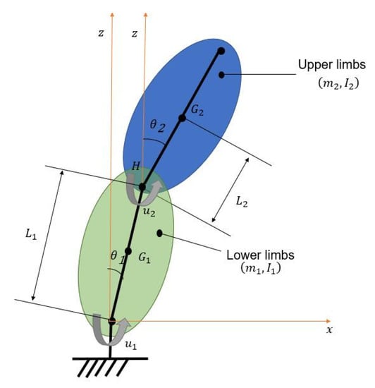
Figure 4.
A human posture inverted pendulum model.
According to [41], the table of human standing model parameters is given as Table 2. Using the data of Table 2, the relevant parameters and matrices can be obtained
Table 2.
Human standing model parameters [41].
It is known that the of NSS (41) contains the compound function and . Therefore, we can obtain SPFM by using the Algorithm 1. The specific steps are as follows:
- The variable transformation. We introduce six new variables , , , , , and .
- Derivative.
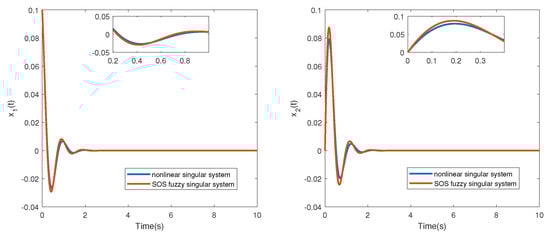
To illustrate the accuracy of the SPFM approximation, the state trajectory and error are given when .
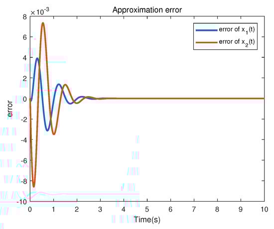
The contrast of state trajectory between human standing system and the SPFM is given by Figure 5, and the error of and is given by Figure 6. As shown in Figure 5 and Figure 6, the SPFM (43) can effectively approximate the NSS (41).
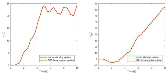
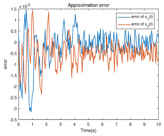
Figure 6.
Approximation error of and .
Remark 9.
As the number of nonlinear items of system (41) is 6, if we use the T-S fuzzy model to approach system (41), the rules of the T-S fuzzy system are at least . If we want to reach about the same accuracy of approximation with the SPFM, the number of fuzzy rules needed is more when using T-S fuzzy model. Therefore, using the SPFM to approach system (41) can effectively reduce the number of fuzzy rules with a high accuracy.
4.2. A Comparison Example with T-S Fuzzy Model
In this subsection, in order to compare the performance of the T-S fuzzy model method, an example of the second-order NSS is considered.
The algorithm processes of SPFM and T-S fuzzy model of system (44) are given below.
- (1)
- SPFM
It is known that system (44) does not contain the compound function and that the nonlinear terms and are bounded except for polynomials. Let and , so , . The membership functions can be calculated
The model rules can be given:
Model Rule 1:
Model Rule 2:
Model Rule 3:
Model Rule 4:
where , , , , , .
Therefore, the SPFM of system (44) is
where , , , .
The error of and is given by Figure 7 when . As shown in Figure 7, system (44) can be approximated system (45) using SPFM effectively.
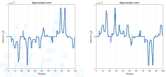
Figure 7.
Approximation error of and using SPFM.
- (2)
- T-S fuzzy model
Let , and , so , and . The membership functions can be calculated
The model rules can be given
Model Rule 1:
Model Rule 2:
Model Rule 3:
Model Rule 4:
Model Rule 5:
Model Rule 6:
Model Rule 7:
Model Rule 8:
where , , , , , , , . Therefore, the T-S fuzzy model of system (44) is
where , , , , , , , .
The errors of and are given in Figure 8 when and using T-S model. The following compares the differences between SPFM and T-S fuzzy model from three aspects (accuracy, number of fuzzy rules, and running time), as shown in the Table 3. By comparison, it can be found that the accuracy of SPFM is much higher than the T-S fuzzy model, and the fuzzy rules of SPFM are half that of T-S fuzzy model. The run time of two models is relatively low, and the time of SPFM is lower than the T-S fuzzy model. Therefore, the approximation effect of SPFM in nonlinear systems is better than the T-S fuzzy model method.
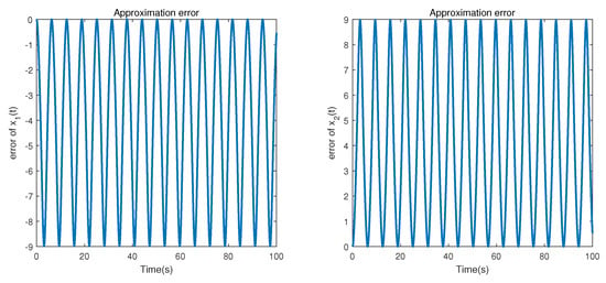
Figure 8.
Approximation error of and using the T-S fuzzy model.
Table 3.
The performance comparison of SPFM and T-S fuzzy model.
4.3. Eliminate Impulse by Using SMC
Consider the SPFM:
where
According to the discrimination method of the singular system impulse, the calculation of matrix rank is given below:
Therefore, the SPFM (47) is impulsive. The objective is to design a linear switching function as in (19) and SMC law (23) such that the closed-loop control system (24) is asymptotically stable. First, the parameter of switching function is given
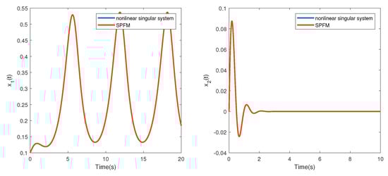
and ; therefore, the matrix M satisfies the design requirement. Then, the parameters of the SMC law (23) are designed with and . Figure 9 shows the state trajectories of SPFM (47) with the initial value . The SMC law and the sliding surface are given as Figure 10 and Figure 11. Figure 9, Figure 10 and Figure 11 show that the states of SPFM (47) converge to zero within 4s under the sliding mode controller (23) and linear sliding mode surface (19), and the SMC laws can eliminate the impulses of SPFM (47).
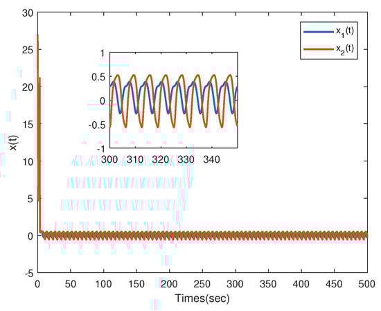
Figure 9.
The state trajectories of system (47).
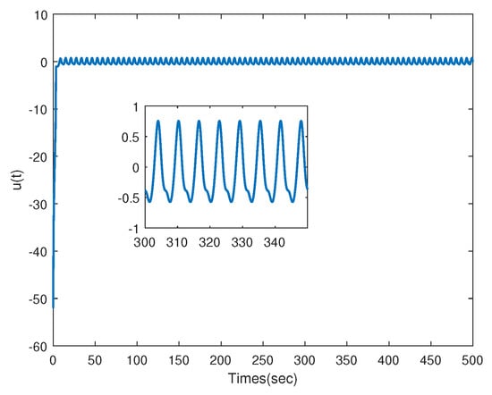
Figure 10.
Sliding mode control law (23).
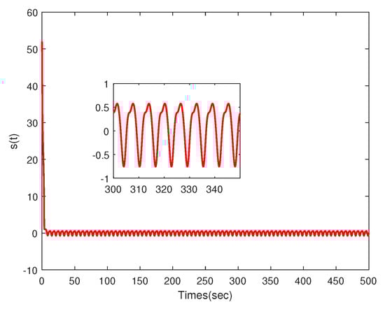
Figure 11.
Linear switching function (19).
5. Conclusions
In this paper, the SPFM approach problem was studied for a class of nonlinear singular system with impulses and without impulses. Consider the nonlinear singular system without impulses; some scholars directly use SOSTOOLS to solve the problem based on the T-S fuzzy model. However, this paper theoretically proves the accuracy of the approximation and gives the algorithm. For the nonlinear singular system with impulses, the theorem of the SPFM that can effectively approach the model has been proven for the first time. It is proved that a class of nonlinear singular system with a bounded impulse-free item property and a separable impulse item property can be approximated by SPFM with arbitrary accuracy. This enables the nonlinear singular system with impulses to be locally linearized with relatively few fuzzy rules and high precision. Then, the designed sliding mode controller can effectively eliminate impulses of the SPFM. Finally, a human posture inverted pendulum model and two numerical example were carried out to demonstrate the effectiveness of the proposed algorithms.
Author Contributions
Conceptualization, J.L. and Y.Z.; methodology, J.L. and Y.Z.; software, Z.J.; validation, J.L. and Y.Z.; formal analysis, J.L. and Y.Z.; investigation, J.L. and Y.Z.; data curation, J.L. and Y.Z.; writing original draft preparation, J.L.; writing review and editing, J.L.; visualization, Z.J.; supervision, Y.Z.; project administration, Y.Z.; funding acquisition, Y.Z. and J.L. All authors have read and agreed to the published version of the manuscript.
Funding
This research was funded by National Natural Science Foundation of China under grant No.61673099.
Institutional Review Board Statement
Not applicable.
Informed Consent Statement
Not applicable.
Data Availability Statement
Not applicable.
Conflicts of Interest
The authors declare no potential conflicts of interest.
References
- Takagi, T.; Sugeno, M. Fuzzy identication of systems and its application to modeling and control. IEEE Trans. Syst. Man Cybern. 1985, 15, 116–132. [Google Scholar] [CrossRef]
- Wang, L.X. Fuzzy systems are universal approximators. In Proceedings of the IEEE International Conference on Fuzzy System, San Diego, CA, USA, 8–12 March 1992; pp. 1153–1162. [Google Scholar]
- Gao, G.S.; Rees, N.W.; Feng, G. Analysis and design for a class of complex control system. Automatica 1997, 33, 1017–1028. [Google Scholar]
- Castro, J.L. Fuzzy logic controllers are universal approximators. IEEE Trans. Syst. Man Cybern. 1995, 25, 629–635. [Google Scholar] [CrossRef]
- Kosko, B. Fuzzy systems as universal approximators. IEEE Trans. Comput. 1994, 43, 1329–1333. [Google Scholar] [CrossRef]
- Ying, H. General Takagi-Sugeno fuzzy systems are universal approximators. In Proceedings of the 1998 IEEE International Conference on Fuzzy Systems Proceedings, IEEE World Congress on Computational Intelligence (Cat. No.98CH36228), Anchorage, AK, USA, 4–9 May 1998; Volume 1, pp. 819–823. [Google Scholar]
- Zeng, X.J.; Singh, M.G. Approximation theory of fuzzy systems-MIMO case. IEEE Trans. Fuzzy Syst. 1995, 3, 219–235. [Google Scholar] [CrossRef]
- Wang, F.; Chen, B.; Sun, Y.M.; Gao, Y.L.; Lin, C. Finite-time fuzzy control of stochastic nonlinear systems. IEEE Trans. Cybern. 2020, 50, 2617–2626. [Google Scholar] [CrossRef]
- Zhang, Y.; Zhang, Q.L.; Zhang, J.Y.; Wang, Y.Y. Sliding-mode control for fuzzy singular systems with time-delay based on vector integral sliding mode surface. IEEE Trans. Fuzzy Syst. 2020, 28, 768–782. [Google Scholar] [CrossRef]
- Tanaka, K.; Yoshida, H.; Ohtake, H.; Wang, H.O. A sum of squares approach to modeling and control of nonlinear dynamical systems with polynomial fuzzy systems. IEEE Trans. Fuzzy Syst. 2009, 17, 911–922. [Google Scholar] [CrossRef]
- Feng, G. A survey on analysis and design of model-based fuzzy control systems. IEEE Trans. Fuzzy Syst. 2006, 14, 676–697. [Google Scholar] [CrossRef]
- Wang, H.O.; Tanaka, K.; Griffen, M.F. An approach to fuzzy control of nonlinear system: Stability and design issues. IEEE Trans. Fuzzy Syst. 1996, 4, 14–23. [Google Scholar] [CrossRef]
- Qiu, J.B.; Feng, G.; Yang, J. A new design of delay-dependent robust H filtering for discrete-time T-S fuzzy systems with time-varying delay. IEEE Trans. Fuzzy Syst. 2009, 17, 1044–1058. [Google Scholar]
- Pang, B.; Zhang, Q.L. Interval observers design for polynomial fuzzy singular systems by utilizing Sum-of-Squares program. IEEE Trans. Syst. Man, Cybern. Syst. 2018, 50, 1–8. [Google Scholar] [CrossRef]
- Pang, B.; Zhang, Q.L. Sliding mode control for polynomial fuzzy singular systems with time delay. IET Control. Theory Appl. 2018, 12, 1483–1490. [Google Scholar] [CrossRef]
- Lam, H.K.; Tsai, S.H. Stability analysis of polynomial-fuzzy-model based control systems with mismatch premise membership functions. IEEE Trans. Fuzzy Syst. 2014, 22, 223–229. [Google Scholar] [CrossRef]
- Lam, H.K. Polynomial fuzzy-model-based control systems: Stability analysis via piecewise-linear membership function. IEEE Trans. Fuzzy Syst. 2011, 19, 588–593. [Google Scholar] [CrossRef]
- Lam, H.K.; Liu, C.; Wu, L.; Zhao, X.D. Polynomial fuzzy-model based control systems: Stability analysis via approximated membership functions considering sector nonlinearity of control input. IEEE Trans. Fuzzy Syst. 2015, 23, 2202–2214. [Google Scholar] [CrossRef]
- Zheng, G.; Boutat, D.; Wang, H. A nonlinear Luenberger-like observer for nonlinear singular systems. Automatica 2017, 86, 11–17. [Google Scholar] [CrossRef]
- Muoi, N.H.; Phat, V.N.; Niamsup, P. Criteria for robust finite-time stabilisation of linear singular systems with interval time-varying delay. IET Control Theory Appl. 2017, 11, 1968–1975. [Google Scholar] [CrossRef]
- Campbell, S.L. Singular Systems of Differential Equations; Pitman: London, UK, 1980. [Google Scholar]
- Singh, S.; Liu, R.W. Existence of state equation representation of linear large-scale dynamical systems. IEEE Trans. Circuit Theory 1973, 20, 239–246. [Google Scholar] [CrossRef]
- Feng, Z.; Shi, Z. Two equivalent sets: Application to singular systems. Automatica 2017, 2017, 198–205. [Google Scholar] [CrossRef]
- Taniguchi, T.; Tanaka, K.; Wang, H.O. Fuzzy descriptor systems and nonlinear model following control. IEEE Trans. Fuzzy Syst. 2000, 8, 442–452. [Google Scholar] [CrossRef]
- Lin, C.; Wang, Q.G.; Lee, T.H. Stability and stabilization of a class of fuzzy time-delay descriptor systems. IEEE Trans. Fuzzy Syst. 2006, 14, 542–551. [Google Scholar]
- Zhai, D.; An, L.W.; Li, J.H.; Zhang, Q.L. Fault detection for stochastic parameter-varing Markovian jump systems with application to networked control systems. Appl. Math. Model. 2016, 40, 2368–2383. [Google Scholar] [CrossRef]
- Wu, J.R. Robust stabilization for uncertain T-S fuzzy singular system. Int. J. Mach. Learn. Cybern. 2016, 7, 699–706. [Google Scholar] [CrossRef]
- Li, W.X.; Feng, Z.G.; Sun, W.C.; Zhang, J.W. Admissibility analysis for Takagi-Sugeno fuzzy singular systems with time delay. Neurocomputing 2016, 205, 336–340. [Google Scholar] [CrossRef]
- Wang, Y.Y.; Zhang, J.Y.; Zhang, H.G. Sliding-mode control for fuzzy stochastic systems with different local input matrices. IEEE Trans. Syst. Man Cybern. Syst. 2019, 51, 4761–4772. [Google Scholar] [CrossRef]
- Wang, Y.Y.; Zhang, J.Y.; Zhang, H.G.; Sun, J.Y. A new stochastic sliding-mode design for descriptor fuzzy systems with time-varying delay. IEEE Trans. Cybern. 2019, 51, 3858–3870. [Google Scholar] [CrossRef]
- Rachunkova, I. Singular Dirichlet second-order BVPs with impulses. J. Differ. Equ. 2003, 193, 435–459. [Google Scholar] [CrossRef][Green Version]
- Zhang, Z.H.; Yuan, R. An application of variational methods to Dirichlet boundary value problem with impulses. Nonlinear Anal. Real World Appl. 2010, 11, 155–162. [Google Scholar] [CrossRef]
- Juan, J.N. Variational formulation of a damped Dirichlet impulsive problem. Appl. Math. Lett. 2010, 23, 940–942. [Google Scholar]
- Utkin, V. Discussion aspects of high-order sliding mode control. IEEE Trans. Autom. Control 2016, 61, 829–833. [Google Scholar] [CrossRef]
- Incremona, G.P.; Rubagotti, M.; Ferrara, A. Sliding mode control of constrained nonlinear systems. IEEE Trans. Autom. Control 2017, 62, 2965–2972. [Google Scholar] [CrossRef]
- Utkin, V. Sliding Modes in Control and Optimization; Springer: Berlin/Heidelberg, Germany, 1992; pp. 12–13. [Google Scholar]
- Lam, H.K.; Narimani, M.; Li, H.; Liu, H. Stability analysis of Polynomial-Fuzzy-Model-Based control systems using switching polynomial Lyapunov function. IEEE Trans. Fuzzy Syst. 2013, 21, 800–813. [Google Scholar] [CrossRef]
- Beardmore, R.E. Double singularity-induced bifurcation points and singular Hopf bifurcations. Dyn. Stab. Syst. 2000, 15, 319–342. [Google Scholar] [CrossRef]
- Ma, J.F.; Zhang, Q.L. Approximation property of T-S fuzzy singular systems. Control. Theory Appl. 2008, 25, 837–844. [Google Scholar]
- Uezato, E.; IkedaStrict, M. LMI conditions for stability, robust stabilization, and H-infity control of descriptor systems. IEEE Conf. Decis. Control 1999, 4, 4092–4097. [Google Scholar]
- Guelton, K.; Delprat, S.; Guerra, T.M. An alternative to inverse dynamics joint torques estimation in human stance based on a Takagi-Sugeno unknown-inputs observer in the descriptor form. Control. Eng. Pract. 2008, 16, 1414–1428. [Google Scholar] [CrossRef]


Publisher’s Note: MDPI stays neutral with regard to jurisdictional claims in published maps and institutional affiliations. |
© 2021 by the authors. Licensee MDPI, Basel, Switzerland. This article is an open access article distributed under the terms and conditions of the Creative Commons Attribution (CC BY) license (https://creativecommons.org/licenses/by/4.0/).