
The Censored Beta-Skew Alpha-Power Distribution


Abstract
:1. Introduction
2. Asymmetric Distributions and Distributions for Multimodal Data
2.1. The Alpha-Power Family of Distributions
2.2. Distributions for Multimodal Data
Properties of the BSN Model
- If , then its cdf is given bytherefore, the survival function, for is given bywhere is the survival function of the standard normal distribution. Likewise, the Hazard function is determined bywhere the Hazard function of the standard normal distribution.
- If , then the pdf can have up to three modes, that is, this distribution is trimodal. In addition, if , then the distribution is bimodal.
- From Proposition 2 of Shafiei et al. [21] one can see that, If , the odd and even order moments of Z, are given byrespectively.
- Consider and denote by and the coefficients of the asymmetry and kurtosis of Z, respectively; then, using (10) and (11) and following Shafiei et al. [21], one can prove that
- (a)
- (b)
- (c)
- (d)
2.3. The Beta-Skew-Alpha-Power Model
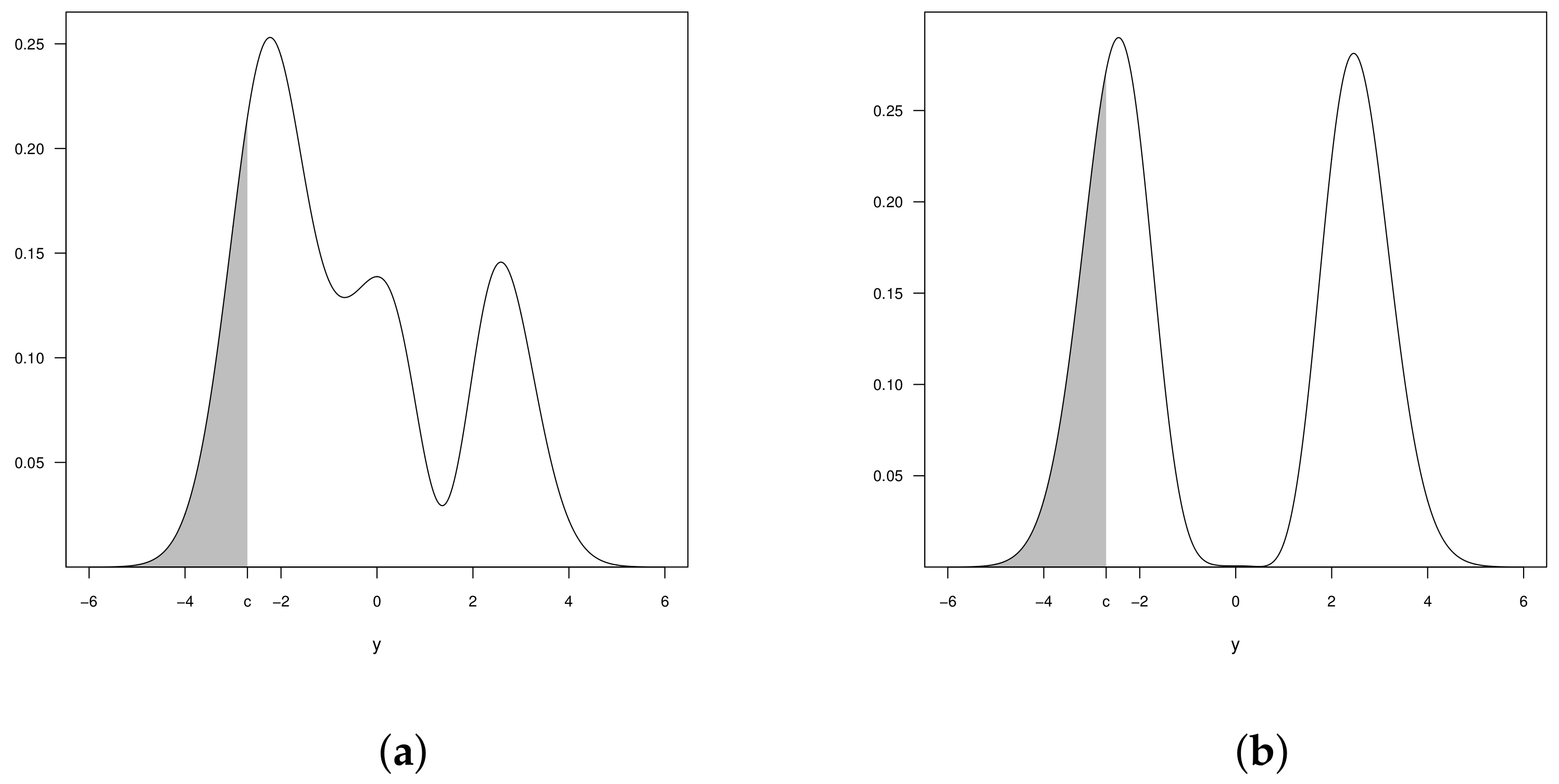
2.4. Censored Beta-Skew-Normal Model
2.5. Moments of the CBSN Model
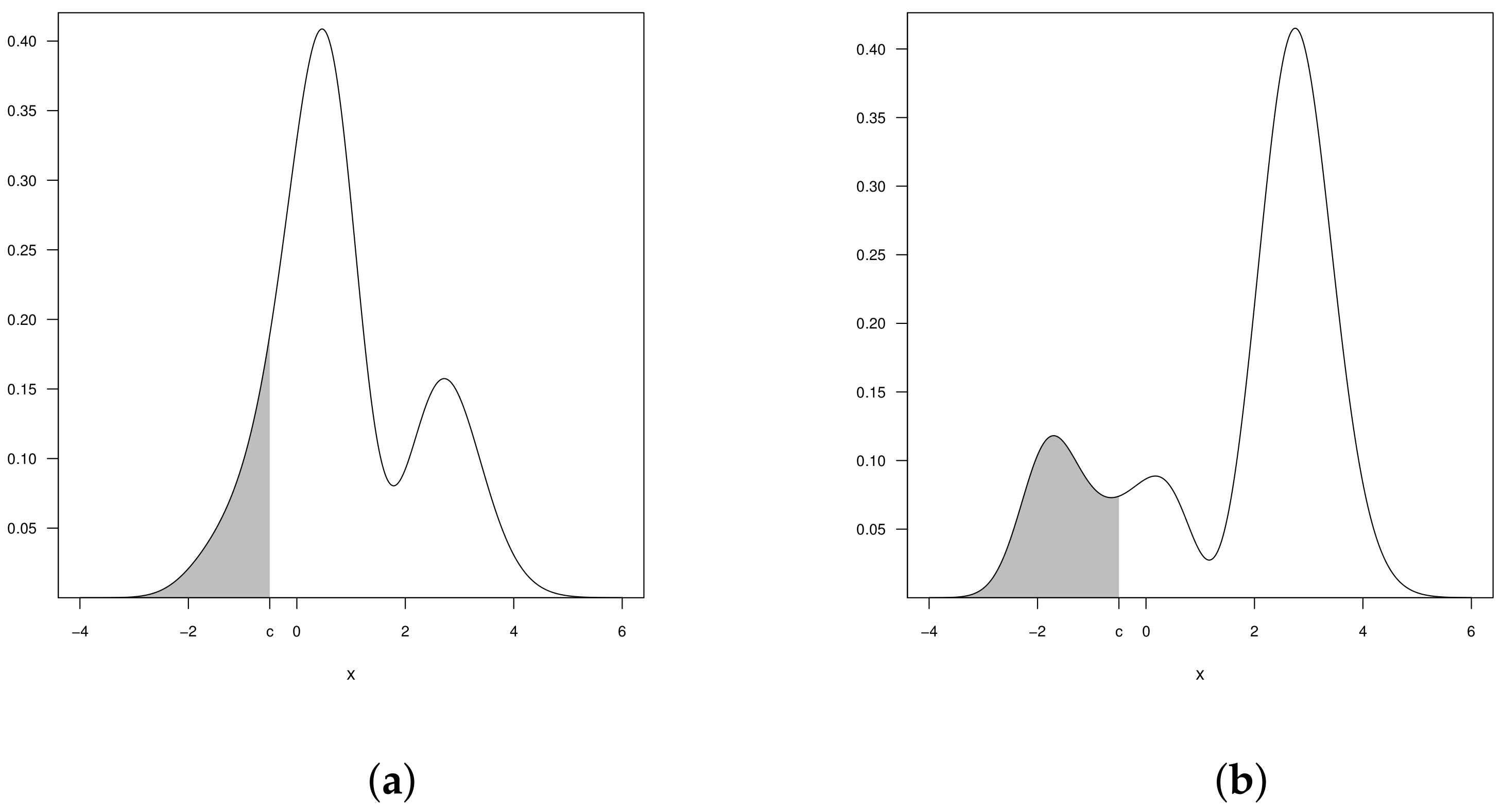
3. Censored Beta-Skew Alpha-Power Model
3.1. Inference for the CBSAP Model
3.2. Model for Positive Data
4. Illustrations
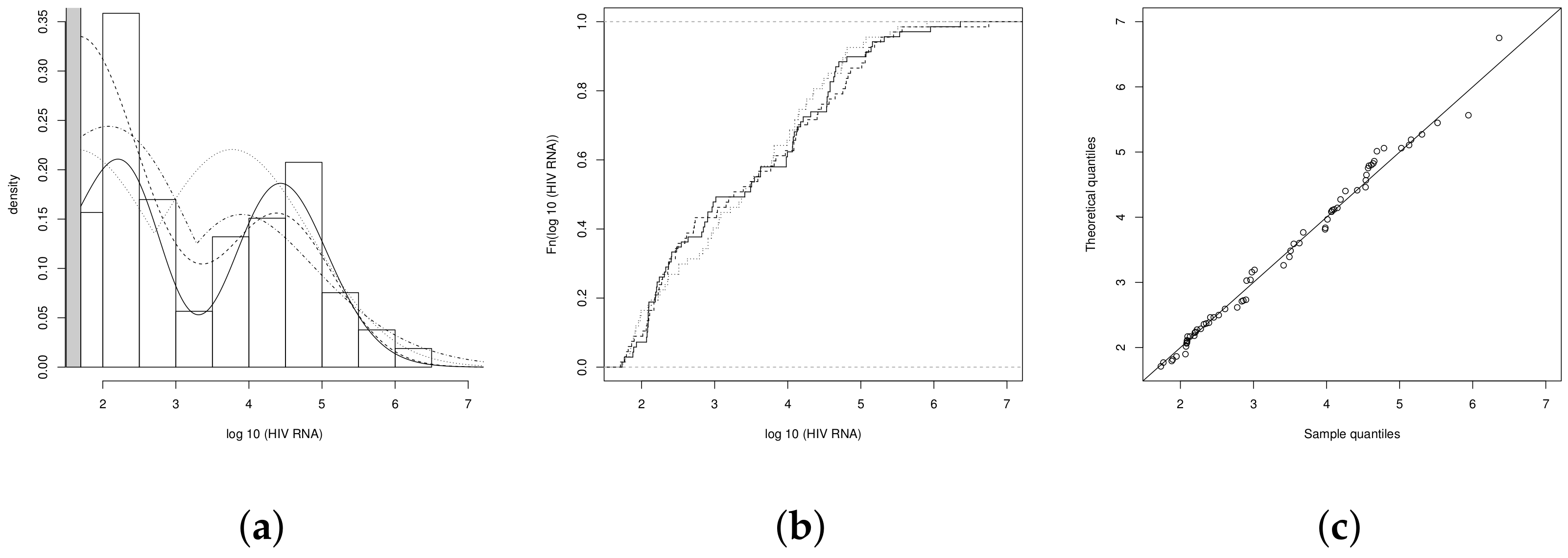
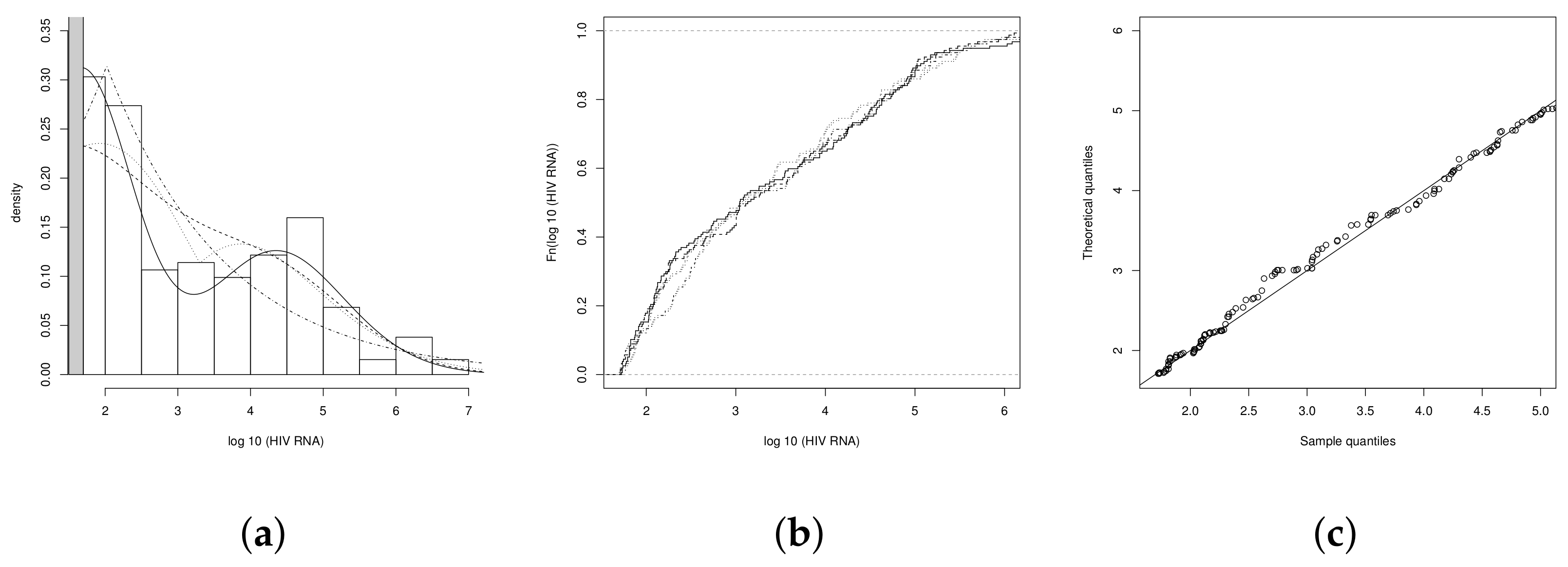
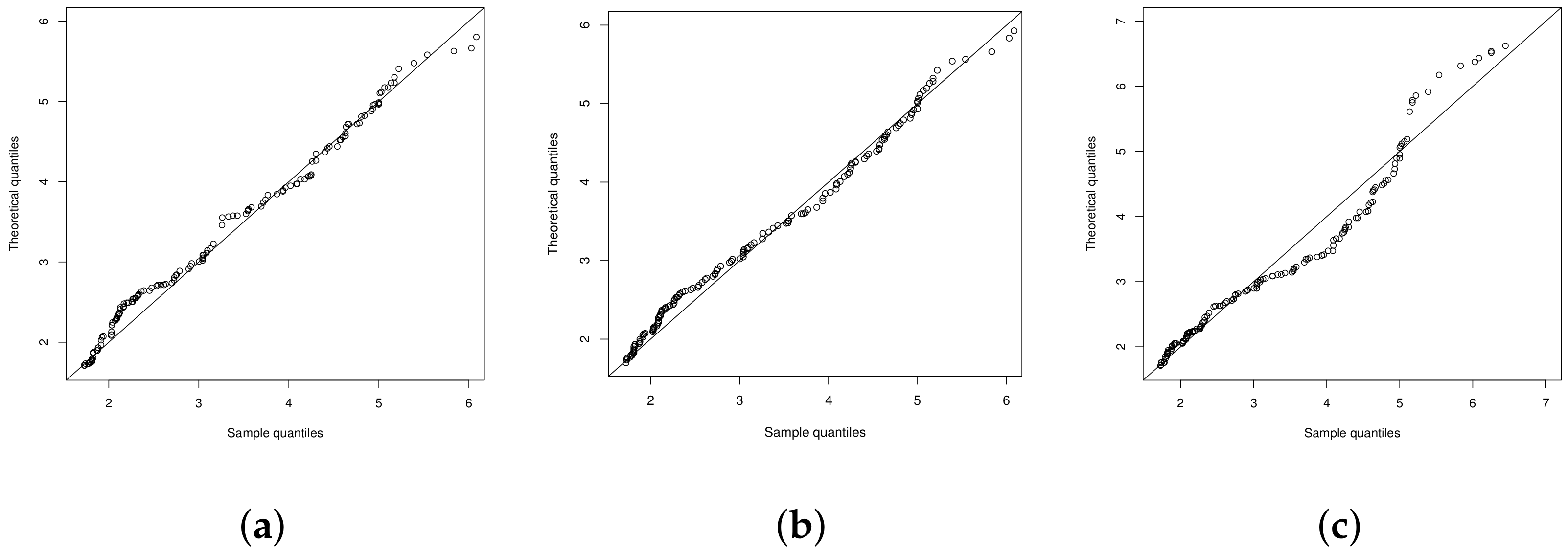
4.1. Illustration 1: The RNA-HIV Data
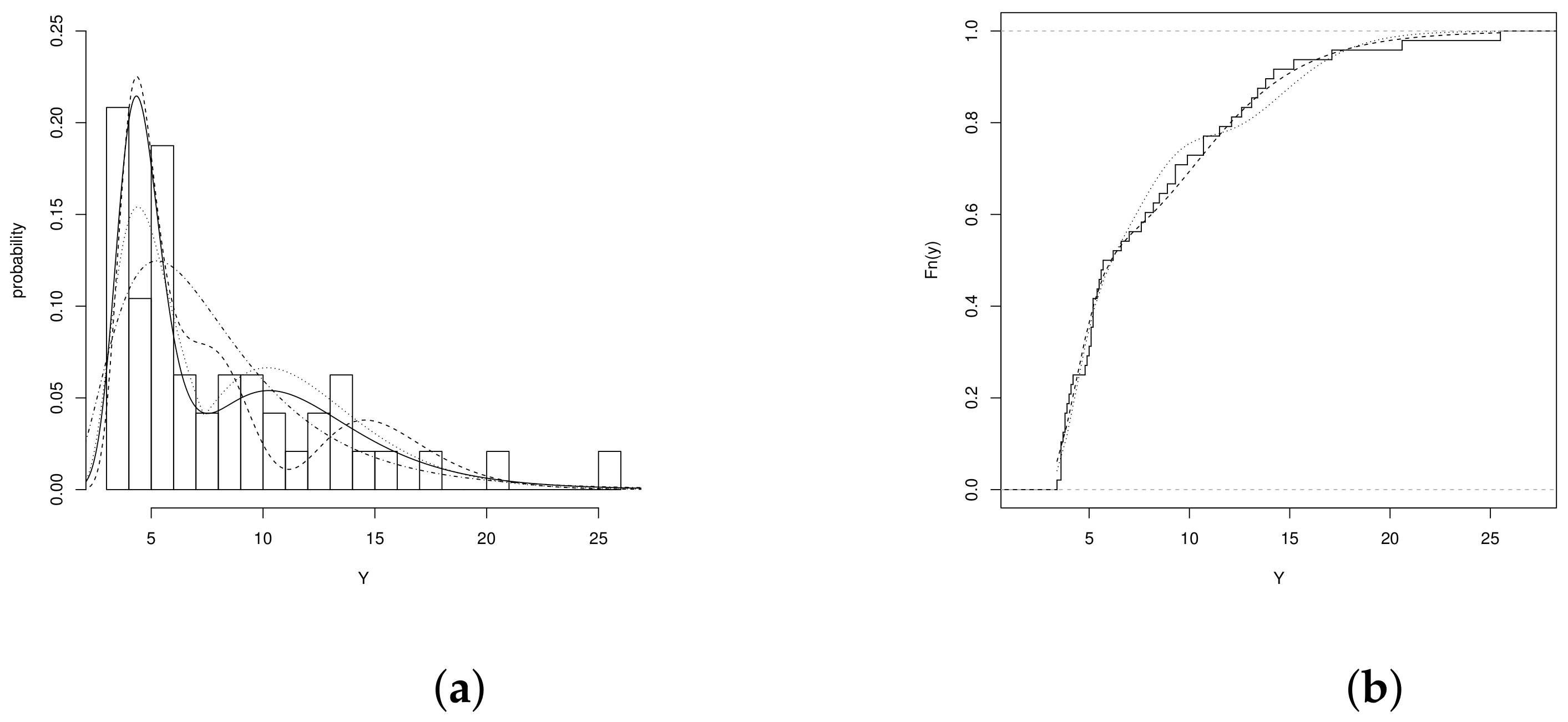
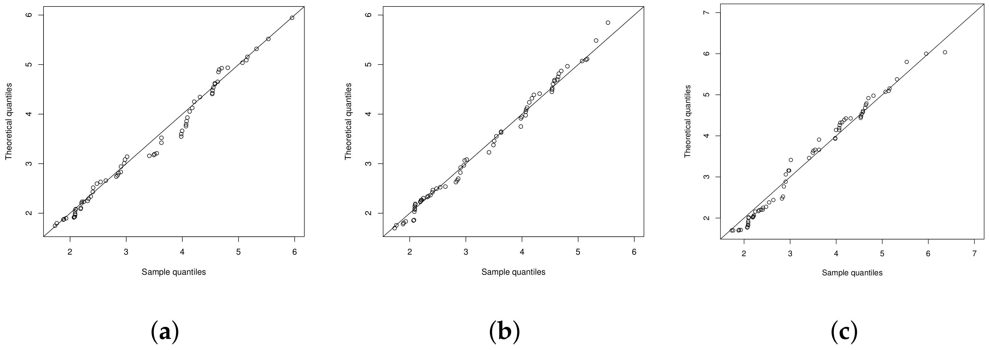
4.2. Illustration 2
4.3. Illustration 3
5. Conclusions
Author Contributions
Funding
Institutional Review Board Statement
Informed Consent Statement
Data Availability Statement
Acknowledgments
Conflicts of Interest
Appendix A
Appendix B. Information Matrix for the CBSAP Model
Appendix B.1. Observed Information Matrix
Appendix B.2. Expected Fisher Information Matrix
References
- Moulton, L.H.; Halsey, N.H. A mixture model with detection limits for regression analyses of antibody response to vaccine. Biometrics 1995, 51, 1570–1578. [Google Scholar] [CrossRef]
- Tobin, J. Estimation of relationships for limited dependent variables. Econometrica 1958, 26, 24–36. [Google Scholar] [CrossRef] [Green Version]
- Martínez-Flórez, G.; Bolfarine, H.; Gómez, H.W. Asymmetric regression models with limited responses with an application to antibody response to vaccine. Biom. J. 2013, 55, 156–172. [Google Scholar] [CrossRef] [PubMed]
- Arellano-Valle, R.; Castro, L.; González-Farías, G.; Muñoz-Gajardo, K. Student-t censored regression model: Properties and inference. Stat. Methods Appl. 2012, 21, 453–473. [Google Scholar] [CrossRef]
- Martínez-Flórez, G.; Bolfarine, H.; Gómez, H.W. The alpha-power tobit model. Commun. -Stat.-Theory Methods 2013, 42, 633–643. [Google Scholar] [CrossRef]
- Chen, T.; Ma, S.; Kobie, J.; Rosenberg, A.; Sanz, I.; Liang, H. Identification of significant B cell associations with undetected observations using a Tobit model. Stat. Interface 2016, 9, 79–91. [Google Scholar] [CrossRef]
- Li, X.; Chu, H.; Gallant, J.E.; Hoover, D.R.; Mack, W.J.; Chmiel, J.S.; Muñoz, A. Bimodal virological response to antiretroviral therapy for HIV infection: An application using a mixture model with left censoring. J. Epidemiol. Community Health 2006, 60, 811–818. [Google Scholar] [CrossRef] [Green Version]
- Marin, J.M.; Mengersen, K.; Robert, K.P. Bayesian modelling and inference on mixtures of distributions. Handb. Stat. 2005, 25, 459–507. [Google Scholar]
- Gómez, H.W.; Elal-Olivero, D.; Salinas, H.S.; Bolfarine, H. Bimodal extension based on the skew-normal distribution with application to pollen data. Environmetrics 2011, 22, 50–62. [Google Scholar] [CrossRef]
- Bolfarine, H.; Martínez-Flórez, G.; Salinas, H.S. Bimodal symmetric-asymmetric power-normal families. Commun. -Stat.-Theory Methods 2018, 47, 259–276. [Google Scholar] [CrossRef]
- Martínez-Flórez, G.; Bolfarine, H.; Gómez, H.W. Censored bimodal symmetric-asymmetric families. Stat. Its Interface 2019, 11, 237–249. [Google Scholar] [CrossRef]
- Azzalini, A. A class of distributions which includes the normal ones. Scand. J. Stat. 1985, 12, 171–178. [Google Scholar]
- Lehmann, E.L. The power of rank tests. Ann. Math. Stat. 1953, 24, 23–43. [Google Scholar] [CrossRef]
- Pewsey, A.; Gómez, H.W.; Bolfarine, H. Likelihood-based inference for power distributions. Test 2012, 21, 775–789. [Google Scholar] [CrossRef]
- Durrans, S.R. Distributions of fractional order statistics in hydrology. Water Resour. Res. 1992, 28, 1649–1655. [Google Scholar] [CrossRef]
- Gupta, R.D.; Gupta, R.C. Analyzing skewed data by power normal model. Test 2008, 17, 197–210. [Google Scholar] [CrossRef]
- Elal-Olivero, D. Alpha-skew-normal distribution. Proyecciones J. Math. 2010, 29, 224–240. [Google Scholar] [CrossRef] [Green Version]
- Kim, H.J. On a class of two-piece skew-normal distributions. Stat. J. Theor. Appl. Stat. 2005, 39, 537–553. [Google Scholar] [CrossRef]
- Arnold, B.C.; Gómez, H.W.; Salinas, H.S. On multiple constraint skewed models. Stat. J. Theor. Appl. Stat. 2009, 43, 273–293. [Google Scholar] [CrossRef]
- Ma, Y.; Genton, M.G. Flexible class of skew-symmetric distributions. Scand. J. Stat. 2004, 31, 459–468. [Google Scholar] [CrossRef] [Green Version]
- Shafiei, S.; Doostparast, M.; Jamalizadeh, A. The alpha–beta skew normal distribution: Properties and applications. Statistics 2016, 50, 338–349. [Google Scholar] [CrossRef]
- Martínez-Flórez, G.; Tovar-Falón, R.; Jimémez-Narváez, M. Likelihood-based inference for the asymmetric beta-skew alpha-power distribution. Symmetry 2020, 12, 613. [Google Scholar] [CrossRef]
- Jäntschi, L.; Bálint, D.B.; Bolboacs, S.D. Multiple linear regressions by maximizing the likelihood under assumption of generalized Gauss-Laplace distribution of the error. Comput. Math. Methods Med. 2016, 2016, 1–8. [Google Scholar] [CrossRef] [PubMed]
- Azzalini, A.; Cappello, T.; Kotz, S. Log-skew-normal and log-skew-t distributions as models for family income data. J. Income Distrib. 2002, 11, 12–20. [Google Scholar]
- Martínez-Flórez, G.; Bolfarine, H.; Gómez, H.W. The log-power-normal distribution with application to air pollution. Environmetrics 2014, 25, 44–56. [Google Scholar] [CrossRef]
- Tovar-Falón, R.; Bolfarine, H.; Martínez-Flórez, G. The Asymmetric Alpha-Power Skew-t Distribution. Symmetry 2020, 12, 82. [Google Scholar] [CrossRef] [Green Version]
- Akaike, H. A new look at statistical model identification. IEEE Trans. Autom. Control. 1974, AU-19, 716–722. [Google Scholar] [CrossRef]
- Schwarz, G. Estimating the dimension of a model. IAnn. Stat. 1978, 6, 461–464. [Google Scholar] [CrossRef]
- Jäntschi, L. A test detecting the outliers for continuous distributions based on the cumulative distribution function of the data being tested. Symmetry 2019, 1, 835. [Google Scholar] [CrossRef] [Green Version]
- Jäntschi, L. Detecting extreme values with order statistics in samples from continuous distributions. Mathematics 2020, 8, 216. [Google Scholar] [CrossRef] [Green Version]
- R Development Core Team. R: A Language and Environment for Statistical Computing; R Foundation for Statistical Computing: Vienna, Austria, 2020; Available online: http://www.R-project.org (accessed on 10 January 2021).
- Ehsani, M.R.; Saadatmanesh, H.; Tao, S. Design recommendations for bond of GFRP rebars to concrete. J. Struct. Eng. 1996, 122, 247–254. [Google Scholar] [CrossRef]
- Olmos, N.M.; Martínez-Flórez, G.; Bolfarine, H. Bimodal Birnbaum–Saunders distribution with applications to non negative measurements. Commun. Stat. -Theory Methods 2017, 46, 6240–6257. [Google Scholar] [CrossRef]


| 1.6488 | 1.7328 | 0.5213 | 2.1315 |
| Estimates | CFN | CETN | CBSN | CBSAP |
|---|---|---|---|---|
| 0.322 (0.006) | 1.603 (0.120) | −0.125 (0.128) | −1.201 (0.431) | |
| 11.778 (1.060) | 2.031 (0.154) | 1.297 (0.074) | 1.383 (0.119) | |
| 7.273 (0.005) | 2.232 (0.865) | −0.205 (0.031) | 0.195 (0.033) | |
| −0.766 (0.146) | 5.637(2.192) | |||
| AIC | 831.87 | 811.89 | 812.43 | 800.23 |
| BIC | 842.59 | 826.18 | 823.15 | 814.52 |
| 1.7112 | 1.4249 | 0.3549 | 1.9836 |
| Estimates | CFN | CETN | CBSAP |
|---|---|---|---|
| 1.006 (0.137) | 1.587 (0.160) | 0.131 (0.297) | |
| 1.079 (0.213) | 1.840 (0.213) | 0.954 (0.101) | |
| −0.987 (0.379) | 2.261 (1.508) | 0.353 (0.060) | |
| −0.588 (0.199) | 2.175 (0.547) | ||
| AIC | 340.95 | 338.63 | 334.61 |
| BIC | 348.95 | 349.29 | 345.27 |
| n | Mean | Variance | Median |
|---|---|---|---|
| 48 |
| Estimates | LN | BSB | LBSN | LBSAP |
|---|---|---|---|---|
| 1.940 (0.076) | 0.317 (0.050) | 2.077 (0.045) | 1.103 (0.169) | |
| 0.528 (0.053) | 7.380 (0.330) | 0.252 (0.016) | 0.469 (0.056) | |
| −1.307 (0.372) | 0.441 (0.083) | 0.216 (0.046) | ||
| 7.893 (3.141) | ||||
| 265.3 | 260.0 | 263.6 | 258.2 | |
| 269.0 | 265.6 | 272.2 | 265.6 |
Publisher’s Note: MDPI stays neutral with regard to jurisdictional claims in published maps and institutional affiliations. |
© 2021 by the authors. Licensee MDPI, Basel, Switzerland. This article is an open access article distributed under the terms and conditions of the Creative Commons Attribution (CC BY) license (https://creativecommons.org/licenses/by/4.0/).
Share and Cite
Martínez-Flórez, G.; Tovar-Falón, R.; Martínez-Guerra, M. The Censored Beta-Skew Alpha-Power Distribution. Symmetry 2021, 13, 1114. https://doi.org/10.3390/sym13071114
Martínez-Flórez G, Tovar-Falón R, Martínez-Guerra M. The Censored Beta-Skew Alpha-Power Distribution. Symmetry. 2021; 13(7):1114. https://doi.org/10.3390/sym13071114
Chicago/Turabian StyleMartínez-Flórez, Guillermo, Roger Tovar-Falón, and María Martínez-Guerra. 2021. "The Censored Beta-Skew Alpha-Power Distribution" Symmetry 13, no. 7: 1114. https://doi.org/10.3390/sym13071114
APA StyleMartínez-Flórez, G., Tovar-Falón, R., & Martínez-Guerra, M. (2021). The Censored Beta-Skew Alpha-Power Distribution. Symmetry, 13(7), 1114. https://doi.org/10.3390/sym13071114