Holomorphic Extensions Associated with Fourier–Legendre Series and the Inverse Scattering Problem

Abstract

In this paper, we consider the inverse scattering problem and, in particular, the problem of reconstructing the spectral density associated with the Yukawian potentials from the sequence of the partial-waves $f_{\ell }$ of the Fourier–Legendre expansion of the scattering amplitude. We prove that if the partial-waves $f_{\ell }$ satisfy a suitable Hausdorff-type condition, then they can be uniquely interpolated by a function $\tilde{f}\left(\lambda \right)\in \mathbb{C}$, analytic in a half-plane. Assuming also the Martin condition to hold, we can prove that the Fourier–Legendre expansion of the scattering amplitude converges uniformly to a function $f\left(\theta \right)\in \mathbb{C}$ ($\theta$ being the complexified scattering angle), which is analytic in a strip contained in the $\theta$-plane. This result is obtained mainly through geometrical methods by replacing the analysis on the complex $cos\theta$-plane with the analysis on a suitable complex hyperboloid. The double analytic symmetry of the scattering amplitude is therefore made manifest by its analyticity properties in the $\lambda$- and $\theta$-planes. The function $f\left(\theta \right)$ is shown to have a holomorphic extension to a cut-domain, and from the discontinuity across the cuts we can iteratively reconstruct the spectral density $\sigma \left(\mu \right)$ associated with the class of Yukawian potentials. A reconstruction algorithm which makes use of Pollaczeck and Laguerre polynomials is finally given.

1. Introduction

In the mathematical theory of the potential scattering, the inverse problem (at fixed energy) may be formulated as follows (see [1]):

Problem 1.

Let

$$\underline{f}(cosu)=\frac{1}{4\pi }\sum _{\ell =0}^{\infty }(2\ell +1)f_{\ell }{P}_{\ell }(cosu),$$

(1)

be the normalized Fourier–Legendre expansion of the scattering amplitude, $P_{\ell }(·)$ being the Legendre polynomials.

Then, given a class $\mathcal{V}$ of potentials, we have the following questions:

(i)

Does there exist a potential $V\in \mathcal{V}$ that generates the sequence of partial-waves ${\left\{f_{\ell }\right\}}_{\ell =0}^{\infty }$?

(ii)

Is this potential unique?

(iii)

Does this potential depend continuously upon the given data ${\left\{f_{\ell }\right\}}_0^{\infty }$?

(iv)

Can we set up an algorithm for recovering this potential from the observations? Can we show its convergence accounting also for that the actual data are either affected by noise and finite in number?

(v)

Can we provide stability estimates for this algorithm?

Here we approach this problem assuming that $\mathcal{V}$ is the class of Yukawian potentials. A Yukawian potential is represented by a spherically symmetric function on ${\mathbb{R}}^3$ of the following form:

$$V_{{\mu }_0}\left(r\right)=\frac{1}{r}{\int }_{{\mu }_0}^{\infty }{e}^{-\mu r}\sigma \left(\mu \right)\mathrm{d}\mu ({\mu }_0>0).$$

(2)

In the past sixties, various authors, in particular Martin and Targonski [2], were able to give a positive answer to the second question (i.e., the question of the uniqueness) for this class of potentials. The same authors gave also a necessary, but in general not sufficient, condition on the coefficients $f_{\ell }$ to guarantee the existence of the potential; hereafter, this condition will be called the M.T. condition.

The question of the existence of the potential, i.e., point (i) above, can be split into two parts:

(a)

The existence of the spectral density $\sigma \left(\mu \right)$ in (2), associated with the partial-waves $f_{\ell }$ and the Legendre expansion (1).

(b)

The convergence of integral (2), which gives $V_{{\mu }_0}\left(r\right)$ when $\sigma \left(\mu \right)$ has been determined from data.

Part (a) of this question can actually be solved by seeking for conditions on the partial-waves ${\left\{f_{\ell }\right\}}_{\ell ={\ell }_0}^{\infty }$ which are sufficient to guarantee a holomorphic extension of series (1) to a suitable slit-domain in $\mathbb{C}$. This connection becomes clear if we recall that the convergence properties of expansion (1), as described, for instance, by Walsh [3], are strictly analogous to the well-known convergence properties of Taylor series. In the Fourier–Legendre expansions, the region of convergence, instead of being the disk of radius $\rho$ of the Taylor series, is an ellipse $E_{\rho }$ with foci in $\pm 1$ and radius $\rho \doteq$(semi-minor+semi-major)-axis. The Legendre expansion converges inside the largest ellipse within which the scattering amplitude $f\left(\theta \right)$ is holomorphic ($\theta \in \mathbb{C}$ being the complexified scattering angle). The main aim of this paper is to prove that if the partial-waves ${\left\{f_{\ell }\right\}}_{\ell =0}^{\infty }$ (or a subset of them) satisfy a suitable Hausdorff-type condition, then the scattering amplitude $f\left(\theta \right)=\underline{f}(cos\theta )$ admits an analytic continuation to the whole complex $\theta$-plane cut from ${\mu }_0$ to $+\infty$. Then, the spectral density $\sigma \left(\mu \right)$ can be iteratively reconstructed by starting from the jump function which describes the discontinuity of $f\left(\theta \right)$ across the cut. Furthermore, it is worth observing that, adopting this setting, it is possible to give a suggestive probabilistic interpretation of the Hausdorff conditions and of the partial-waves $f_{\ell }$. More precisely, we will see in Section 2.2 that the partial-waves $f_{\ell }$ can be regarded as the values of a harmonic function associated with a suitable Markov process. Part (b) of question (i) remains still unanswered.

Concerning question (iii) the answer is negative: the inverse scattering problem (at fixed energy) is known to be ill-posed in the sense of Hadamard, with the data $f_{\ell }$ being necessarily affected by noise and, furthermore, the experiments can provide only a finite number of them. Nevertheless, in [4] (see also [5]) it has been proposed an algorithm, based on the Pollaczek polynomials, which is able to reconstruct iteratively the spectral density $\sigma \left(\mu \right)$ starting from a finite set of noisy data ${\left\{f_{\ell }^{\left(\epsilon \right)}\right\}}_{\ell =0}^L$ (or ${\left\{f_{\ell }^{\left(\epsilon \right)}\right\}}_{\ell ={\ell }_0}^L$), where $\epsilon$ characterizes some kind of bound on the noise. It was furthermore possible to evaluate stability estimates and to prove that the approximation error, associated with the numerical algorithm, tends to zero in the topology of the $L^2$-norm, as the number of data tends to infinity and the bound $\epsilon$ on the noise tends to zero. We can thus say that the questions (iii) and (v) listed above, have received a quite satisfactory answer in [4]. However, that paper presents some limits and essentially two main defects:

(i)

The condition imposed on the partial-waves was unnecessarily restrictive.

(ii)

The holomorphic extension associated with the Fourier–Legendre series (1) was only conjectured but not rigorously proved.

One of the purposes of the present paper is indeed to remedy these defects. First (see Section 2.1), we introduce an appropriate Hausdorff-type condition on the partial-waves which allows us to prove that the set of the partial-waves admit a unique Carlsonian interpolant. Then, we study the Hardy space to which this interpolant belongs. In Section 2.2 we give the probabilistic interpretation of the Hausdorff condition in terms of Markov processes. Next, we obtain the holomorphic extension of the scattering amplitude $f\left(\theta \right)$ to the cut $cos\theta$-plane, whose proof is performed in various steps. The first step consists in replacing the complex $cos\theta$-plane ($\theta \in \mathbb{C}$) with a complex hyperboloid $X^{\left(c\right)}$. The hyperboloid $X^{\left(c\right)}$ contains the following submanifolds: the Euclidean sphere ${\mathbb{S}}_2=(\mathrm{i}\mathbb{R}\times {\mathbb{R}}^2)\cap X^{\left(c\right)}$ where the $SO(3,\mathbb{R})$ harmonic analysis is done, and the real one-sheteed hyperboloid $X={\mathbb{R}}^3\cap X^{\left(c\right)}$ that contains the cut support. The second step is a fibration on a meridian hyperbola of $X^{\left(c\right)}$, implemented by means of a Radon-type transformation where the role played by the planes in the ordinary Radon transformation is now played by the horocycles. By this fibration, we can thus to reduce the harmonic analysis on the complex hyperboloid to that on a complex one-dimensional hyperbola, which contains the Euclidean circle and the real hyperbola. In this way, series (1) can be regarded as a trigonometrical series on the Euclidean circle. This last step is proved in Appendix A, while the geometrical method we used is illustrated in Appendix B. Once the trigonometrical series is obtained, we can prove that it admits a holomorphic extension to a complex cut-plane. This is proved in Section 3. Finally, in Section 4 we return back to the complex $cos\theta$-plane (i.e., the complex hyperboloid $X^{\left(c\right)}$) by inverting the Radon transformation, and finally prove the analytic extension of the Fourier–Legendre series (1). The inversion of the Radon transform is analyzed in Appendix C. The unique interpolation of the coefficients ${\left\{f_{\ell }\right\}}_{\ell =0}^{\infty }$ turns out to be a Laplace-type transform (precisely, the composition of Laplace and Radon transformations) of the jump across the cut. Therefore, by inverting this transformation, we can reconstruct the discontinuity function which leads to the spectral density $\sigma \left(\mu \right)$. This latter step is described in Section 5. In the same section we briefly show how the jump function across the cuts can be reconstructed by means of the Pollaczek polynomials. Finally, Section 6 is devoted to the analysis of the connection between the first order Born approximation of the scattering amplitude and the Laplace-composed-with-Radon transform, introduced in Appendix C.

2. Interpolation of Hausdorff Moments and Hardy Spaces

2.1. Hausdorff Moments and Hardy Spaces

Let ${\mathbb{N}}_0$ denote the non-negative integers: ${\mathbb{N}}_0=\mathbb{N}\cup \left\{0\right\}$ and ${\mathbb{C}}_{-1/2}^{(+)}$ the complex half-plane: ${\mathbb{C}}_{-1/2}^{(+)}=\{\lambda \in \mathbb{C},\mathrm{Re}\lambda >-\frac{1}{2}\}$. Consider a sequence ${\left\{a_{\ell }\right\}}_{\ell =0}^{\infty }$ of (real) numbers $a_{\ell }$, and denote by $\Delta$ the difference operator

$$\Delta a_{\ell }=a_{\ell +1}-a_{\ell }.$$

(3)

Then we have:

$${\Delta }^k{a}_{\ell }=\underset{k\mathrm{times}}{\underbrace{\Delta \times \Delta \times \cdots \times \Delta }}{a}_{\ell }=\sum _{m=0}^k{(-1)}^m\left(\genfrac{}{}{0pt}{}{k}{m}\right)a_{\ell +k-m},$$

(4)

(for every $k⩾0$); ${\Delta }^0$ is the identity operator, by definition. Now, suppose that there exists a positive constant M such that:

$${(\ell +1)}^{(1+\epsilon )}\sum _{i=0}^{\ell }{\left(\genfrac{}{}{0pt}{}{\ell }{i}\right)}^{(2+\epsilon )}{\left|{\Delta }^i{a}_{(\ell -i)}\right|}^{(2+\epsilon )}<M(\ell \in {\mathbb{N}}_0;\epsilon >0).$$

(5)

We shall refer to (5) as the Hausdorff condition in view of its relevance for the solution of the Hausdorff moment problem. In fact, it can be proved [6] that condition (5) is necessary and sufficient to represent the numbers $a_{\ell }$, $\ell \in {\mathbb{N}}_0$, as moments of a suitable function, that is:

$$a_{\ell }={\int }_0^1{x}^{\ell }u\left(x\right)\mathrm{d}x(\ell \in {\mathbb{N}}_0),$$

(6)

where $u\left(x\right)\in L^{2+\epsilon }(0,1)$. Next, the tool we use to guarantee the uniqueness of the interpolation of a sequence of numbers is Carlson’s theorem [7].

Theorem 1

(Carlson’s theorem [7] (§9.2, p. 153)). Let $a\left(\lambda \right)$ be regular in the complex half-plane $\mathrm{Re}\lambda ⩾0$ and

(i) 

$a\left(\lambda \right)$ is of exponential type $\tau <\infty$,

(ii) 

$a\left(\mathrm{i}y\right)=O\left(1\right)exp\left(c\right|y\left|\right)$ for some $c<\pi$ ($y=\mathrm{Im}\lambda$),

(iii) 

$a(\ell )=0$ for $\ell =0,1,2,\dots$,

then $a\left(\lambda \right)$ vanishes identically.

We shall refer to conditions (i) and (ii) as Carlson’s bound. Moreover, an analytic function which interpolates a sequence of numbers ${\left\{f_{\ell }\right\}}_{\ell =0}^{\infty }$ and satisfy conditions (i) and (ii) above will be called a Carlsonian interpolant.

Now, we can prove the following proposition (see also [8] for a preliminary version of this proposition).

Proposition 1.

For $p⩾1$, let the sequence ${\left\{a_{\ell }^{\left(p\right)}\right\}}_{\ell =0}^{\infty }$, with $a_{\ell }\doteq {(\ell +1)}^p{f}_{\ell }$, satisfy condition (5). Then, there exists a unique Carlsonian interpolant $\tilde{f}\left(\lambda \right)$ ($\lambda \in \mathbb{C}$, $\mathrm{Re}\lambda ⩾-\frac{1}{2}$) of the sequence ${\left\{f_{\ell }\right\}}_{\ell =0}^{\infty }$, i.e., $\tilde{f}{\left(\lambda \right)|}_{\lambda =\ell }=f_{\ell }$ for $\ell \in {\mathbb{N}}_0$, which satisfies the following conditions:

(i) 

$\tilde{f}\left(\lambda \right)$ is holomorphic in the half-plane $\mathrm{Re}\lambda >-\frac{1}{2}$, continuous at $\mathrm{Re}\lambda =-\frac{1}{2}$ and belongs to the Hardy space $H^2\left({\mathbb{C}}_{-1/2}^{(+)}\right)$;

(ii) 

${\lambda }^p\tilde{f}\left(\lambda \right)$ belongs to $L^2(-\infty ,+\infty )$ for any fixed value of $\mathrm{Re}\lambda ⩾-\frac{1}{2}$;

(iii) 

${\lambda }^p\tilde{f}\left(\lambda \right)$ tends uniformly to zero as $\lambda \to \infty$ inside any fixed half-plane $\mathrm{Re}\lambda ⩾\delta >-\frac{1}{2}$;

(iv) 

${\lambda }^{(p-1)}\tilde{f}\left(\lambda \right)$ belongs to $L^1(-\infty ,+\infty )$ for any fixed value of $\mathrm{Re}\lambda ⩾-\frac{1}{2}$.

Proof. 

If the sequence ${\left\{a_{\ell }\right\}}_0^{\infty }$ satisfies condition (5), then representation (6) holds true and, putting $x=e^{-t}$ in the integral, it gives:

$$a_{\ell }={\int }_0^{\infty }{e}^{-\ell t}{e}^{-t}u\left(e^{-t}\right)\mathrm{d}t(\ell \in {\mathbb{N}}_0),$$

(7)

with $u\in L^{2+\epsilon }(0,1)$, $\epsilon >0$. The numbers $a_{\ell }$ can thus be viewed as the restriction to ${\mathbb{N}}_0$ of the following Laplace transform:

$$\tilde{a}\left(\lambda \right)={\int }_0^{\infty }{e}^{-(\lambda +1/2)t}{e}^{-t/2}u\left(e^{-t}\right)\mathrm{d}t(\mathrm{Re}\lambda >-\frac{1}{2}).$$

(8)

In fact, we have: $\tilde{a}{\left(\lambda \right)|}_{\lambda =\ell }=a_{\ell }$. Applying the Paley–Wiener theorem to (8) and observing that $exp(-t/2)u(exp(-t\left)\right)$ belongs to $L^2(0,+\infty )$ since $u\in L^{2+\epsilon }(0,1)$, we can conclude that $\tilde{a}\left(\lambda \right)$ belongs to the Hardy space $H^2\left({\mathbb{C}}_{-1/2}^{(+)}\right)$ whose norm is: ${\parallel \tilde{a}\parallel }_2\doteq {sup}_{\sigma >-1/2}({\int }_{-\infty }^{\infty }|\tilde{a}(\sigma +\mathrm{i}\nu ){{|}^2\mathrm{d}\nu )}^{1/2}$. In view of the Carlson theorem, we can state that $\tilde{a}\left(\lambda \right)$ is the unique Carlsonian interpolant of the sequence ${\left\{a_{\ell }\right\}}_0^{\infty }$. Now, define $\tilde{f}\left(\lambda \right)\doteq \tilde{a}\left(\lambda \right)/{(\lambda +1)}^p$. Then, $\tilde{f}\left(\lambda \right)$ is holomorphic for $\mathrm{Re}\lambda >-\frac{1}{2}$ and satisfies the Carlson bound since $\tilde{a}\left(\lambda \right)$ does. Hence, $\tilde{f}\left(\lambda \right)$ is the unique Carlsonian interpolant of the set of Fourier–Legendre coefficients ${\left\{f_{\ell }\right\}}_0^{\infty }$ since $\tilde{f}{\left(\lambda \right)|}_{\lambda =\ell }={\left.\frac{\tilde{a}\left(\lambda \right)}{{(\lambda +1)}^p}\right|}_{\lambda =\ell }=\frac{a_{\ell }}{{(\ell +1)}^p}=f_{\ell }$. Moreover, $\tilde{f}\left(\lambda \right)\in H^2\left({\mathbb{C}}_{-1/2}^{(+)}\right)$, in fact:

$${\parallel \tilde{f}\parallel }_2^2=\underset{\sigma >-\frac{1}{2}}{sup}{\int }_{-\infty }^{\infty }{\left|\frac{\tilde{a}(\sigma +\mathrm{i}\nu )}{{(\sigma +1+\mathrm{i}\nu )}^p}\right|}^2\mathrm{d}\nu ⩽16\underset{\sigma >-\frac{1}{2}}{sup}{\int }_{-\infty }^{\infty }{\left|\tilde{a}(\sigma +\mathrm{i}\nu )\right|}^2\mathrm{d}\nu <\infty .$$

(9)

Next, by using the Hölder inequality, we see that $e^{-t/2}u\left(e^{-t}\right)\in L^1(0,+\infty )$:

$$\begin{array}{cc}\hfill & {\int }_0^{\infty }\left|e^{-t/2}u\left(e^{-t}\right)\right|\mathrm{d}t={\int }_0^1|u\left(x\right)/\sqrt{x}|\mathrm{d}x\hfill \\ & ⩽{\left({\int }_0^1{\left|u\left(x\right)\right|}^{(2+\epsilon )}\mathrm{d}x\right)}^{\frac{1}{2+\epsilon }}{\left({\int }_0^1{x}^{-\frac{2+\epsilon }{2+2\epsilon }}\mathrm{d}x\right)}^{\frac{1+\epsilon }{2+\epsilon }}<\infty ,\hfill \end{array}$$

(10)

for the rightmost integral converges since $\frac{2+\epsilon }{2+2\epsilon }<1$ for $\epsilon >0$, and $u\in L^{(2+\epsilon )}(0,1)$. Then, for the Riemann–Lebesgue theorem applied to representation (8) at $\mathrm{Re}\lambda =-\frac{1}{2}$, it follows that both functions $\tilde{a}(-1/2+\mathrm{i}\nu )$ and $\tilde{f}(-1/2+\mathrm{i}\nu )$, $(\nu \in \mathbb{R})$, are continuous. Property (i) is thus proved. Property (ii) follows from $\tilde{a}\in H^2\left({\mathbb{C}}_{-1/2}^{(+)}\right)$, which implies $\tilde{a}(\sigma +\mathrm{i}\nu )\in L^2(-\infty ,\infty )$ for any fixed value of $\sigma ⩾-\frac{1}{2}$. Concerning point (iii), since $\tilde{a}\left(\lambda \right)\in H^2\left({\mathbb{C}}_{-1/2}^{(+)}\right)$, then $\tilde{a}\left(\lambda \right)$ tends to zero as $\lambda \to \infty$ inside any half-plane $\mathrm{Re}\lambda ⩾\delta >-\frac{1}{2}$. Regarding property (iv), by Schwartz’s inequality, we have for $\sigma ⩾-\frac{1}{2}$ and $p⩾1$:

$$\begin{array}{cc}& {\int }_{-\infty }^{\infty }\left|{(\sigma +\mathrm{i}\nu )}^{p-1}\tilde{f}(\sigma +\mathrm{i}\nu )\right|\mathrm{d}\nu ={\int }_{-\infty }^{\infty }\left|{(\sigma +\mathrm{i}\nu )}^{p-1}\frac{\tilde{a}(\sigma +\mathrm{i}\nu )}{{(\sigma +1+\mathrm{i}\nu )}^p}\right|\mathrm{d}\nu \hfill \\ & ⩽{\left({\int }_{-\infty }^{\infty }{\left|\frac{{(\sigma +\mathrm{i}\nu )}^{p-1}}{{(\sigma +1+\mathrm{i}\nu )}^p}\right|}^2\mathrm{d}\nu \right)}^{1/2}{\left({\int }_{-\infty }^{\infty }{\left|\tilde{a}(\sigma +\mathrm{i}\nu )\right|}^2\mathrm{d}\nu \right)}^{1/2}<\infty ,\hfill \end{array}$$

(11)

since $\tilde{a}(\sigma +\mathrm{i}\nu )\in L^2(-\infty ,+\infty )$ for any fixed value of $\sigma ⩾-1/2$. □

2.2. Hausdorff Moments and Markov Processes

In this subsection we follow the paper of Watanabe [9]. Let $(\Omega ,\mathcal{F},P)$ be an abstract probability field. If $\{y_{\ell }\left(\tilde{\omega }\right);\ell ⩾1\}$ is a sequence of mutually independent random variables on $(\Omega ,\mathcal{F},P)$ and each random variable satisfies

$$P\{y_{\ell }\left(\tilde{\omega }\right)=1\}=p\mathrm{and}P\{y_{\ell }\left(\tilde{\omega }\right)=0\}=1-p,$$

(12)

then this sequence is called a Bernoulli sequence and will be denoted by $B\left(p\right)$. In particular, in what follows we shall consider $B(1/2)$. Let E be the set of all couples $(\ell ,i)$ such that $\ell ⩾i$; $\ell ,i\in {\mathbb{N}}_0$. Next, we consider the discrete Markov process $x_{\ell }$, conservative over E, which corresponds to the stochastic matrix of the transition probabilities: ${\Pi }^{\ell }((\ell ,i),(\ell +1,i))={\Pi }^{\ell }((\ell ,i),(\ell +1,i+1)=\frac{1}{2})$. It is called the discrete Markov process $x_{\ell }$ attached to $B(1/2)$ since this process can be derived from the Bernoulli sequence $B(1/2)$. Let us note that

$$P_{(\ell ,i)}\{x_k=(m,j)\}=\left\{\begin{array}{cc}{\displaystyle \phantom{(}{\left(\frac{1}{2}\right)}^k\left(\genfrac{}{}{0pt}{}{k}{j-i}\right)}\hfill & \mathrm{for}m=\ell +k,j⩾i,\hfill \\ 0\hfill & \mathrm{otherwise},\hfill \end{array}\right.$$

(13)

where $k⩾0$, $(\ell ,i),(m,j)\in E$. The kernel $K\left(\right(\ell ,i),(m,j\left)\right)$ is given by:

$$K((\ell ,i),(m,j))=\frac{P_{(\ell ,i)}\{\sigma \left(\{m,j\}\right)<\infty \}}{P_{(0,0)}\{\sigma \left(\{m,j\}\right)<\infty \}}=2^{\ell }\frac{(m-\ell )!j!(m-j)!}{m!(m-\ell -j+i)!(j-i)!},$$

(14)

$\sigma (·)$ denoting the Markov time. Now, consider an infinite sequence $(m_k,j_k)$ having no limit points in E such that

$$\underset{k\to \infty }{lim}\frac{j_k}{m_k}=1-b,$$

(15)

for a suitable $0⩽b⩽1$. Then, by the Stirling formula and taking into account equality (15), from (14) we obtain:

$$K((\ell ,i),b)=2^{\ell }{b}^{(\ell -i)}{(1-b)}^i.$$

(16)

Thus, the Martin boundary $\mathcal{M}$ (see [10,11]) which is induced by the process $x_{\ell }$ coincides with the interval $[0,1]$ as a set. Hence, the generalized Poisson kernel $K\left(\right(\ell ,i),b)$ is given by $2^{\ell }{b}^{(\ell -i)}{(1-b)}^i$. We finally observe that for a function u defined on E the expectation $E_{(0,0)}$ is given by:

$$E_{(0,0)}\left(\right|u\left(x_{\ell }\right)\left|\right)=2^{-\ell }\sum _{i=0}^{\ell }\left(\genfrac{}{}{0pt}{}{\ell }{i}\right)\left|u(\ell ,i)\right|.$$

(17)

Then, the following propositions proved by Watanabe [9] can be stated.

Proposition 2.

Let $x_{\ell }$ be the Markov process attached to the Bernoulli sequence $B(1/2)$. Then,

(i) 

The Martin boundary induced by the process $x_{\ell }$ is equivalent to the interval $[0,1]$ with the ordinary topology.

(ii) 

The generalized Poisson kernel $K\left(\right(\ell ,i),b)$ is:

$$K((\ell ,i),b)=2^{\ell }{b}^{(\ell -i)}{(1-b)}^i.$$

(18)

(iii) 

Every non-negative function u which belongs to the set of all the finite real-valued functions over $E^{☆}\doteq E\cup \infty$ vanishing at ∞, can be represented by a bounded signed measure on $\left([0,1],{\mathcal{B}}_{[0,1]}\right)$, where ${\mathcal{B}}_{[0,1]}$ is the Borel field composed of all the ordinary Borel subsets in $[0,1]$, that is:

$$u(\ell ,i)=2^{\ell }{\int }_0^1{b}^{(\ell -i)}{(1-b)}^{i}d\mu \left(b\right)\forall (\ell ,i)\in E,$$

(19)

if and only if u is $x_{\ell }$-harmonic and $E_{(0,0)}\left(\right|u\left(x_{\ell }\right)\left|\right)$ is bounded with respect to ℓ.

Proposition 3.

Let $x_{\ell }$ be the Markov process attached to the Bernoulli sequence $B(1/2)$. Given a sequence of real numbers ${\left\{a_{\ell }\right\}}_{\ell =0}^{\infty }$ such that:

$$\sum _{i=0}^{\ell }\left(\genfrac{}{}{0pt}{}{\ell }{i}\right)\left|{\Delta }^i{a}_{(\ell -i)}\right|<L(\forall \ell \in {\mathbb{N}}_0),$$

(20)

then the function

$$u(\ell ,i)\doteq 2^{\ell }{(-1)}^i{\Delta }^i{a}_{(\ell -i)},$$

(21)

is a $x_{\ell }$-harmonic function and can be represented by Formula (19).

It is worth noting that from representation (19) it follows that

$$2^{-\ell }u(\ell ,0)={\int }_0^1{b}^{\ell }d\mu \left(b\right),$$

(22)

which can be compared with representation (6). Moreover, if the sequence ${\left\{a_{\ell }\right\}}_{\ell =0}^{\infty }$ satisfies bound (5), then satisfies inequality (20) too. If inequality (5) is satisfied then the following relationship holds true:

$$(\ell +1)\sum _{i=0}^{\ell }{\left(\genfrac{}{}{0pt}{}{\ell }{i}\right)}^2{\left|{\Delta }^i{a}_{(\ell -i)}\right|}^2<M(\ell =0,1,2,\dots ).$$

(23)

Hence, if in the Cauchy inequality

$$\sum _{i=0}^n\left|{\alpha }_i{\beta }_i\right|⩽{\left(\sum _{i=0}^n{\left|{\alpha }_i\right|}^2\right)}^{1/2}{\left(\sum _{i=0}^n{\left|{\beta }_i\right|}^2\right)}^{1/2},$$

(24)

We put: ${\beta }_i=1$ and ${\alpha }_i=\left(\genfrac{}{}{0pt}{}{\ell }{i}\right)\left|{\Delta }^i{a}_{(\ell -i)}\right|$, $\forall i\in (0,1,2,\dots ,\ell )$, we obtain:

$$\sum _{i=0}^{\ell }\left(\genfrac{}{}{0pt}{}{\ell }{i}\right)\left|{\Delta }^i{a}_{(\ell -i)}\right|⩽{(\ell +1)}^{1/2}{\left[\sum _{i=0}^{\ell }{\left(\genfrac{}{}{0pt}{}{\ell }{i}\right)}^2{\left|{\Delta }^i{a}_{(\ell -i)}\right|}^2\right]}^{1/2}.$$

(25)

Therefore, from inequalities (23) and (25) we obtain:

$$\sum _{i=0}^{\ell }\left(\genfrac{}{}{0pt}{}{\ell }{i}\right)\left|{\Delta }^i{a}_{(\ell -i)}\right|⩽\frac{\sqrt{M}}{{(\ell +1)}^{1/2}}{(\ell +1)}^{1/2}=\sqrt{M},$$

(26)

that coincides with inequality (20) if we put $L=\sqrt{M}$.

3. Holomorphic Extension Associated with the Trigonometrical Series

In Appendix A we show that a series expansion in terms of Legendre polynomials $P_{\ell }(cosu)$ can be regarded as a trigonometrical series, i.e., as a series of the type $\frac{1}{2\pi }{\sum }_{\ell =0}^{\infty }{f}_{\ell }{e}^{-i\ell t}$ (see Formulae (A3), (A4) and (A19)). Then, it is quite natural to introduce the complex plane $\mathbb{C}$ of the variable $\tau =t+iw$, ($t,w\in \mathbb{R}$), and consider in this plane the following domains (see also [12]). For ${\xi }_0⩾0$ we define: ${\mathcal{I}}_{+}^{(\pm {\xi }_0)}\doteq \{\tau \in \mathbb{C}\mid \mathrm{Im}\tau >\pm {\xi }_0\}$, and ${\mathcal{I}}_{-}^{(\pm {\xi }_0)}\doteq \{\tau \in \mathbb{C}\mid \mathrm{Im}\tau <\pm {\xi }_0\}$. Correspondingly, we introduce the cut-domains: ${\mathcal{I}}_{+}^{\left({\xi }_0\right)}\setminus {\Xi }_{+}^{\left({\xi }_0\right)}$, where ${\Xi }_{+}^{\left({\xi }_0\right)}\doteq \{\tau \in \mathbb{C}\mid \tau =2k\pi +iww>{\xi }_{0}k\in \mathbb{Z}\}$ (see Figure 1a) and ${\mathcal{I}}_{-}^{(-{\xi }_0)}\setminus {\Xi }_{-}^{(-{\xi }_0)}$, where ${\Xi }_{-}^{(-{\xi }_0)}\doteq \{\tau \in \mathbb{C}\mid \tau =2k\pi +iw,w<-{\xi }_{0}k\in \mathbb{Z}\}$ (see Figure 1b). Moreover, we will use the notation $\dot{A}=A\setminus 2\pi \mathbb{Z}$ to denote every subset A of $\mathbb{C}$ which is invariant under the translation group $2\pi \mathbb{Z}$.

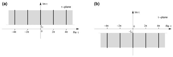
Figure 1. In the complex $\tau$-plane, the grey regions represent: (a) the cut-domain ${\mathcal{I}}_{+}^{\left({\xi }_0\right)}\setminus {\Xi }_{+}^{\left({\xi }_0\right)}$, (b) the cut-domain ${\mathcal{I}}_{-}^{(-{\xi }_0)}\setminus {\Xi }_{-}^{(-{\xi }_0)}$. The cuts (thick lines) are located at $\mathrm{Re}\tau =2k\pi$, $k\in \mathbb{Z}$.

We can then prove the following theorem (see also [8]).

Theorem 2.

Consider the following series:

$$\frac{1}{2\pi }\sum _{\ell =0}^{\infty }{f}_{\ell }{e}^{-i\ell \tau }(\tau =t+iw;t,w\in \mathbb{R}),$$

(27)

and suppose that the set of numbers ${\left\{a_{\ell }\right\}}_{\ell =0}^{\infty }$, $a_{\ell }={(\ell +1)}^p{f}_{\ell }$, $(p⩾1,\ell \in {\mathbb{N}}_0)$, satisfies condition (5). Then,

(1) 

The series (27) converges uniformly on any compact subdomain of ${\mathcal{I}}_{-}^{\left(0\right)}$ to a function $\widehat{f}\left(\tau \right)$, analytic in ${\mathcal{I}}_{-}^{\left(0\right)}$ and continuous on the axis $\mathrm{Im}\tau =0$.

(2) 

The function $\widehat{f}\left(\tau \right)$ can be holomorphically extended to the cut-domain ${\mathcal{I}}_{+}^{\left(0\right)}\setminus {\dot{\Xi }}_{+}^{\left(0\right)}$ (see Figure 1a), that is, it is analytic in $\mathbb{C}\setminus \{\tau \in \mathbb{C}:\tau =2k\pi +\mathrm{i}w;k\in \mathbb{Z},w>0\}$.

(3) 

The jump function $\widehat{F}\left(w\right)$ describing the discontinuity of $i\widehat{f}\left(\tau \right)$ across the cuts ${\dot{\Xi }}_{+}^{\left(0\right)}$), is a function of class $C^{(p-1)}$ and satisfies the bound:

$$|\widehat{F}\left(w\right)|⩽\parallel {\tilde{f}}_{\sigma }{\parallel }_1{e}^{\sigma w}(\sigma ⩾-\frac{1}{2},w\in {\mathbb{R}}^{+}),$$

(28)

where $\tilde{f}(\sigma +i\nu )$, $(\nu \in \mathbb{R})$, is the unique Carlsonian interpolant of the coefficients $f_{\ell }$, and

$${\parallel {\tilde{f}}_{\sigma }\parallel }_1=\frac{1}{2\pi }{\int }_{-\infty }^{+\infty }\left|\tilde{f}(\sigma +i\nu )\right|\mathrm{d}\nu <\infty (\sigma ⩾-\frac{1}{2}).$$

(29)

(4) 

$\tilde{f}(\sigma +i\nu )$ is the Laplace transform of the jump function $\widehat{F}\left(w\right)$:

$$\tilde{f}(\sigma +\mathrm{i}\nu )={\int }_0^{+\infty }\widehat{F}\left(w\right)e^{-(\sigma +\mathrm{i}\nu )w}\mathrm{d}w(\sigma >-\frac{1}{2}).$$

(30)

(5) 

The following Plancherel equality holds true:

$${\int }_{-\infty }^{+\infty }|\tilde{f}{(\sigma +\mathrm{i}\nu )|}^2\mathrm{d}\nu =2\pi {\int }_0^{+\infty }{\left|\widehat{F}\left(w\right)e^{-\sigma w}\right|}^2\mathrm{d}w(\sigma ⩾-\frac{1}{2}).$$

(31)

Proof. 

Since the set ${\left\{a_{\ell }\right\}}_{\ell =0}^{\infty }$ satisfies condition (5), then, given an arbitrary non-negative number C, there exists an integer m such that for $\ell >m$, $|f_{\ell }|\le C$. Therefore, we can write:

$$\frac{1}{2\pi }\left|\sum _{\ell >m}^{\infty }{f}_{\ell }{e}^{-i\ell \tau }\right|⩽\frac{C}{2\pi }\sum _{\ell >m}^{\infty }{e}^{\ell w}(\tau =t+iw),$$

(32)

the series on the r.h.s. of (32) being uniformly convergent for $w⩽w_0<0$. On the other hand, series (27) can be rewritten as

$$\frac{1}{2\pi }\sum _{\ell =0}^{\infty }{f}_{\ell }{e}^{-i\ell \tau }=\frac{1}{2\pi }\sum _{\ell >m}^{\infty }{f}_{\ell }{e}^{-i\ell \tau }+T_m\left(\tau \right),$$

(33)

where $T_m\left(\tau \right)$ is a trigonometric polynomial. Then, for the Weierstrass theorem on the uniformly convergent series of analytic functions, we can conclude that the series (27) converges uniformly on any compact subdomains of ${\mathcal{I}}_{-}^{\left(0\right)}$ to a function $\widehat{f}\left(\tau \right)$ holomorphic in ${\mathcal{I}}_{-}^{\left(0\right)}$. Moreover, $f_{\ell }=O\left({\ell }^{p+\delta }\right)$, $\delta >0$, since ${(\ell +1)}^p{f}_{\ell }\to 0$ as $\ell \to \infty$. Then, given an arbitrary constant $C^{\prime }$, there exists an integer ${\ell }_1$ such that for $w=0$ we have:

$$\left|\frac{1}{2\pi }\sum _{\ell ={\ell }_1}^{\infty }{f}_{\ell }{e}^{-\mathrm{i}\ell t}\right|⩽\frac{1}{2\pi }\sum _{\ell ={\ell }_1}^{\infty }\left|f_{\ell }\right|⩽\frac{C^{\prime }}{2\pi }\sum _{\ell ={\ell }_1}^{\infty }\frac{1}{{(\ell +1)}^{p+\delta }}<\infty (\delta >0).$$

(34)

Then, using once again the Weierstrass theorem on the uniformly convergent series of continuous functions, the series $\frac{1}{2\pi }{\sum }_{\ell =0}^{\infty }{f}_{\ell }{e}^{-\mathrm{i}\ell t}$ converges to a continuous function $\widehat{f}\left(t\right)$. Hence, the first statement is proved. To prove the other statements, we introduce the following integral:

$${\widehat{f}}_{\eta }\left(t\right)=\frac{\mathrm{i}}{4\pi }{\int }_{\mathcal{C}}\tilde{f}\left(\lambda \right)\frac{e^{-\mathrm{i}\lambda (t-\eta \pi )}}{sin\pi \lambda }\mathrm{d}\lambda (\eta =\pm ),$$

(35)

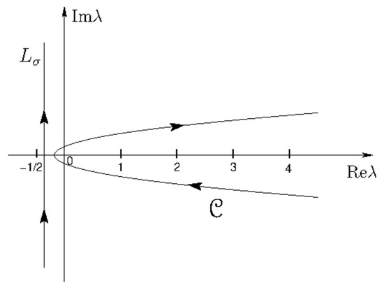
where $\tilde{f}\left(\lambda \right)$, $(\mathrm{Re}\lambda ⩾-\frac{1}{2})$, is the unique Carlsonian interpolant of the sequence ${\left\{f_{\ell }\right\}}_0^{\infty }$, which exists in view of the fact that the set ${\left\{a_{\ell }\right\}}_0^{\infty }$ satisfies condition (5). The contour $\mathcal{C}$ is contained in the half-plane ${\mathbb{C}}_{-1/2}^{(+)}$, encircles the real semi-axis with $\mathrm{Re}\lambda >-\frac{1}{2}$ (or a part of it), and cross this axis at a point $\sigma >-\frac{1}{2}$, $\sigma \notin {\mathbb{N}}_0$, as illustrated in Figure 2.

Figure 2. $\mathcal{C}$ is the integration path of integral (35), which is deformed into $L_{\sigma }$ (see Theorem 2).

Let us now consider the following inequalities, which hold true for any $\sigma ,\nu \in \mathbb{R}$:

$$\begin{array}{cc}\hfill & \left|e^{-\mathrm{i}(\sigma +\mathrm{i}\nu )(t-\pi )}\right|⩽2cosh\pi \nu (t\in [0,2\pi ]),\hfill \end{array}$$

(36)

$$\begin{array}{cc}\hfill & |sin\pi (\sigma +\mathrm{i}\nu \left)\right|⩾sinh\pi \nu ,\hfill \end{array}$$

(37)

$$\begin{array}{cc}\hfill & \left|\frac{e^{-\mathrm{i}(\sigma +i\nu )(t-\pi )}}{sin\pi (\sigma +i\nu )}\right|⩽2\left|\frac{cosh\pi \nu }{sinh\pi \nu }\right|(t\in [0,2\pi ]).\hfill \end{array}$$

(38)

Let us recall that ${\lambda }^p\tilde{f}\left(\lambda \right)$ ($p⩾1$) tends uniformly to zero as $\lambda \to \infty$ inside any fixed half-plane $\mathrm{Re}\lambda ⩾\delta >-1/2$ and, moreover, ${\lambda }^{(p-1)}\tilde{f}\left(\lambda \right)$ belongs to $L^1(-\infty ,+\infty )$ for $\mathrm{Re}\lambda ⩾-1/2$. For these properties and by the use of bound (38), the integral ${\widehat{f}}_{+}\left(t\right)$, $(t\in [0,2\pi \left]\right)$, exists and the contour $\mathcal{C}$ can be deformed and replaced by the line $L_{\sigma }=\{\lambda =\sigma +\mathrm{i}\nu ,\nu \in \mathbb{R},\sigma ⩾-1/2\}$, provided that the real variable $t\in [0,2\pi ]$ (see Figure 2). Hence, by applying the Watson resummation method [13], we obtain for $t\in [0,2\pi ]$:

$${\widehat{f}}_{+}\left(t\right)=-\frac{1}{4\pi }{\int }_{-\infty }^{+\infty }\tilde{f}(\sigma +\mathrm{i}\nu )\frac{e^{-\mathrm{i}(\sigma +\mathrm{i}\nu )(t-\pi )}}{sin\pi (\sigma +\mathrm{i}\nu )}\mathrm{d}\nu =\frac{1}{2\pi }\sum _{\ell ={\ell }_0}^{\infty }{f}_{\ell }{e}^{-\mathrm{i}\ell t},$$

(39)

with ${\ell }_0\in {\mathbb{N}}_0$, $-1/2⩽\sigma <0$ if ${\ell }_0=0$ and ${\ell }_0-1<\sigma <{\ell }_0$ if ${\ell }_0>0$.

Proceeding analogously for the integral ${\widehat{f}}_{-}\left(t\right)$ (Formulae (35) with $\eta =-$), we distort similarly the contour of integration and finally obtain for $t\in [-2\pi ,0]$:

$${\widehat{f}}_{-}\left(t\right)=-\frac{1}{4\pi }{\int }_{-\infty }^{+\infty }\tilde{f}(\sigma +\mathrm{i}\nu )\frac{e^{-\mathrm{i}(\sigma +\mathrm{i}\nu )(t+\pi )}}{sin\pi (\sigma +\mathrm{i}\nu )}\mathrm{d}\nu =\frac{1}{2\pi }\sum _{\ell ={\ell }_0}^{\infty }{f}_{\ell }{e}^{-\mathrm{i}\ell t},$$

(40)

with ${\ell }_0\in {\mathbb{N}}_0$, $-1/2⩽\sigma <0$ if ${\ell }_0=0$ and ${\ell }_0-1<\sigma <{\ell }_0$ if ${\ell }_0>0$.

Now, in integral (39) we substitute for t the complex variable $\tau =t+iw$, and see that the resulting integral provides an analytic continuation of ${\widehat{f}}_{+}\left(t\right)$ in the strip $\{\tau =t+iw,0<t<2\pi ,w\in {\mathbb{R}}^{+}\}$, continuous in the closure of the latter. We have:

$$e^{-\sigma w}{\widehat{f}}_{+}(t+iw)=\frac{1}{2\pi }{\int }_{-\infty }^{+\infty }{H}_{\sigma }^t\left(\nu \right)e^{\mathrm{i}\nu w}\mathrm{d}\nu (\forall \tau =t+iw,0⩽t⩽2\pi ,w\in {\mathbb{R}}_{+}),$$

(41)

with

$$H_{\sigma }^t\left(\nu \right)\doteq -\frac{\tilde{f}(\sigma +\mathrm{i}\nu )e^{-\mathrm{i}(\sigma +\mathrm{i}\nu )(t-\pi )}}{2sin\pi (\sigma +\mathrm{i}\nu )}(\sigma ⩾-\frac{1}{2}),$$

(42)

then, using bound (38), and since ${\lambda }^{(p-1)}\tilde{f}\left(\lambda \right)\in L^1(-\infty ,+\infty )$ for any fixed value of $\mathrm{Re}\lambda =\sigma ⩾-1/2$ (see Proposition 1), the statement is proved. Similarly, the analytic continuation of the function ${\widehat{f}}_{-}$ is defined in the strip $\{\tau =t+iw,-2\pi <t<0\}$. We thus have proved that the function $\widehat{f}\left(\tau \right)$, $(\tau =t+iw)$, admits a holomorphic extension to the cut-domain ${\mathcal{I}}_{+}^{\left(0\right)}\setminus {\dot{\Xi }}_{+}^{\left(0\right)}$. The discontinuity $\mathrm{i}[{\widehat{f}}_{+}\left(\mathrm{i}w\right)-{\widehat{f}}_{-}\left(\mathrm{i}w\right)]$ across the cuts can be computed by replacing t with $\left(\mathrm{i}w\right)$ in integrals (39) and (40). We obtain

$$\widehat{F}\left(w\right)\doteq \mathrm{i}[{\widehat{f}}_{+}\left(\mathrm{i}w\right)-{\widehat{f}}_{-}\left(\mathrm{i}w\right)]=\frac{1}{2\pi }{\int }_{-\infty }^{+\infty }\tilde{f}(\sigma +\mathrm{i}\nu )e^{(\sigma +\mathrm{i}\nu )w}\mathrm{d}\nu (w\in {\mathbb{R}}^{+},\sigma ⩾-\frac{1}{2}).$$

(43)

From (43) we derive the following bound for the jump function $\widehat{F}\left(w\right)$:

$$|\widehat{F}\left(w\right)|⩽\parallel {\tilde{f}}_{\sigma }{\parallel }_1{e}^{\sigma w}(\sigma ⩾-\frac{1}{2},w\in {\mathbb{R}}^{+}),$$

(44)

where $\parallel {\tilde{f}}_{\sigma }{\parallel }_1$, given in (29), is guaranteed to be finite by statement (iv) of Proposition 1. Using Formulae (43) and recalling the Riemann–Lebesgue theorem, we prove that $\widehat{F}\left(w\right)$ is a function of class $C^{(p-1)}$, $(p⩾1)$, since ${\lambda }^{(p-1)}\tilde{f}\left(\lambda \right)\in L^1(-\infty ,+\infty )$ for any $\mathrm{Re}\lambda ⩾-1/2$ (see Proposition 1). Inverting Formulae (43), we have:

$$\tilde{f}\left(\lambda \right)={\int }_0^{+\infty }\widehat{F}\left(w\right)e^{-\lambda w}dw(\mathrm{Re}\lambda >-\frac{1}{2}),$$

(45)

which is the Laplace transform of the jump function $\widehat{F}\left(w\right)$, holomorphic for $\mathrm{Re}\lambda >-1/2$. Finally, recalling that $\tilde{f}(\sigma +\mathrm{i}\nu )$ belongs to $L^2(-\infty ,+\infty )$ for any fixed value $\sigma ⩾-1/2$, we obtain the Plancherel equality (31), which for $\sigma =-\frac{1}{2}$ reads:

$${\int }_{-\infty }^{+\infty }{\left|\tilde{f}(-\frac{1}{2}+\mathrm{i}\nu )\right|}^2\mathrm{d}\nu =2\pi {\int }_0^{+\infty }{\left|\widehat{F}\left(w\right)e^{w/2}\right|}^{2}dw.$$

(46)

□

We can now state the following proposition (see also [8]).

Proposition 4.

If in the trigonometrical series

$$\frac{1}{2\pi }\left(\sum _{\ell =0}^{\infty }{f}_{\ell }{e}^{-\mathrm{i}\ell t}-e^{\mathrm{i}t}\sum _{\ell =0}^{\infty }{f}_{\ell }{e}^{\mathrm{i}\ell t}\right)(t\in \mathbb{R}),$$

(47)

the coefficients $f_{\ell }$ satisfy the assumptions of Theorem 2, then:

(1) 

the series converges to a continuous function $\widehat{f}\left(t\right)$, $(t\in \mathbb{R})$, and the convergence is uniform on any compact subdomain of the real line;

(2) 

the function $\widehat{f}\left(t\right)$ admits a holomorphic extension to the cut-domain ${\dot{\mathcal{I}}}_{\tau }^{\left(0\right)}\doteq \left({\mathcal{I}}_{+}^{\left(0\right)}\setminus {\dot{\Xi }}_{+}^{\left(0\right)}\right)\cup \left({\mathcal{I}}_{-}^{\left(0\right)}\setminus {\dot{\Xi }}_{-}^{\left(0\right)}\right)$ of the τ-plane;

(3) 

the jump function across the cuts ${\dot{\Xi }}_{\pm }^{\left(0\right)}$ enjoys properties strictly analogous to properties (3–5) of Theorem 2.

Proof. 

Statement (1) follows by observing that, in view of the hypothesis on the coefficients $f_{\ell }$, we have:

$$\left|\frac{1}{2\pi }\left(\sum _{\ell =0}^{\infty }{f}_{\ell }{e}^{-\mathrm{i}\ell t}-e^{\mathrm{i}t}\sum _{\ell =0}^{\infty }{f}_{\ell }{e}^{\mathrm{i}\ell t}\right)\right|⩽\frac{1}{\pi }\sum _{\ell =0}^{\infty }\left|f_{\ell }\right|<\infty .$$

(48)

Next, in view of the Weierstrass theorem on the uniformly convergent series of continuous functions, the result follows. Statements (2) and (3) can be proved in a way completely analogous to the one followed for proving the corresponding statements of Theorem 2. □

Suppose now that the partial-waves $f_{\ell }$ satisfy the following bound, which is precisely the M.T. condition [2]:

$$|f_{\ell }|⩽C{e}^{-(\ell -m){\xi }_0}(\ell >m,m\in {\mathbb{R}}^{+},{\xi }_0>0;C=\mathrm{constant}).$$

(49)

From inequality (49) it follows that the series (47) converges to a function $\widehat{f}\left(\tau \right)$, analytic in the strip $\left|\mathrm{Im}\tau \right|<{\xi }_0$, the convergence being uniform in any compact subdomain of this strip. With slight modifications of Theorem 2, it is also straightforward to prove that $\widehat{f}\left(\tau \right)$ admits a holomorphic extension to the cut-domain ${\dot{\mathcal{I}}}_{\tau }^{\left({\xi }_0\right)}\doteq \left({\mathcal{I}}_{+}^{\left(0\right)}\setminus {\dot{\Xi }}_{+}^{\left({\xi }_0\right)}\right)\cup \left({\mathcal{I}}_{-}^{\left(0\right)}\setminus {\dot{\Xi }}_{-}^{(-{\xi }_0)}\right)$ (see Figure 3).

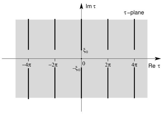
Figure 3. Cut domain ${\dot{\mathcal{I}}}_{\tau }^{\left({\xi }_0\right)}$. It represents the analiticity domain of $\widehat{f}\left(\tau \right)$ when the coefficients $f_{\ell }$ satisfy the Martin condition (49) (see Proposition 4).

The physical applications could also lead to assume that only the subset ${\left\{a_{\ell }\right\}}_{\ell ={\ell }_0}^{\infty }$, $({\ell }_0>0)$, satisfies condition (5). In this case it is easy to prove that $\tilde{f}\left(\lambda \right)$ is analytic in the half-plane $\mathrm{Re}\lambda >{\ell }_0-\frac{1}{2}$, continuous at $\mathrm{Re}\lambda ={\ell }_0-\frac{1}{2}$; furthermore, bound (28) holds for $\sigma ⩾{\ell }_0-\frac{1}{2}$ (instead of $\sigma ⩾-\frac{1}{2}$). Analogous modifications must be introduced in connection with Formulae (30) and (31).

4. Holomorphic Extension Associated with the Legendre Series

In Appendix B we consider a real one-sheteed hyperboloid, denoted by X, and the associated meridian hyperbola, denoted by ${\widehat{X}}^{+}$. Next, we introduce through a Radon transformation a fibration with basis ${\widehat{X}}^{+}$. This Radon transformation allows us to pass from polar coordinates $(\theta ,\varphi )$ to horocyclic coordinates $(\tau ,\zeta )$ (see Appendix B). In this transformation, the horocycles play the same role played by the planes in the ordinary Radon transform. Then, we replace the complex $cos\theta$-plane (see the Introduction) by a complex hyperboloid $X^{\left(c\right)}$, whose submanifolds are the real one-sheteed hyperboloid X and the Euclidean sphere ${\mathbb{S}}_2=(\mathrm{i}\mathbb{R}\times {\mathbb{R}}^2)\cap X^{\left(c\right)}$. Next, we extend the fibration with basis ${\widehat{X}}^{+}$ to the complex hyperboloid $X^{\left(c\right)}$ and to the related complex meridian hyperbola ${\widehat{X}}^{\left(c\right)}$. This fibration is realized by a Radon transform which allows us to pass from the complex polar coordinates $(\theta ,\varphi )$, $(\theta =u+iv)$, to the complex horocyclic coordinates $(\tau ,\zeta )$, $(\tau =t+iw)$. Finally, in Appendix C, we study the inversion of the Radon transformation. By using this latter, we move back from the $\tau$-plane to the $\theta$-plane (see, in particular, representation (A53), which holds if the sequence $a_{\ell }={(\ell +1)}^p{f}_{\ell }$ satisfies the Hausdorff condition (5) with $p⩾2$; see Appendix C). Then, the holomorphic extension in the $\tau$-plane, proved in the previous section, can now be re-formulated in the $\theta$-plane. More precisely, we can state the following propositions.

Proposition 5.

Suppose that the sequence $a_{\ell }={(\ell +1)}^p{f}_{\ell }$ satisfies the Hausdorff condition (5) with $p⩾2$ and let $f\left(\theta \right)$ be the function represented by the following formula (see Appendix C, Formula (A53)):

$$f\left(\theta \right)=\frac{1}{\pi sin\theta }\frac{\mathrm{d}}{\mathrm{d}\theta }{\int }_{{\gamma }_{\theta }}{e}^{-\mathrm{i}\tau /2}\widehat{f}\left(\tau \right)\frac{sin\tau }{{\left[2(cos\theta -cos\tau )\right]}^{1/2}}\mathrm{d}\tau (\theta =u+iv),$$

(50)

where ${\gamma }_{\theta }$ denotes the ray ${\underline{\gamma }}_{\theta }$ oriented from 0 to θ in the τ-plane. Then, $f\left(\theta \right)$ is even, $2\pi$-periodic and holomorphic in ${\dot{\mathcal{I}}}_{\theta }^{\left(0\right)}$.

Proof. 

From the assumptions on $f_{\ell }$ we can state that $\widehat{f}\left(\tau \right)$ is a $2\pi$-periodic function holomorphic in ${\dot{\mathcal{I}}}_{\tau }^{\left(0\right)}$ (see Proposition 4 and Figure 3). Moreover, it satisfies the following symmetry property:

$$\widehat{f}\left(\tau \right)=-e^{\mathrm{i}\tau }\widehat{f}(-\tau ),$$

(51)

which follows from equality (A17) for the uniqueness of the analytic continuation (see Appendix B, Formulae (A41)). These properties imply the $\widehat{f}\left(\tau \right)$ is of the following form: $\widehat{f}\left(\tau \right)=exp(\mathrm{i}\tau /2){(1-cos\tau )}^{1/2}b(cos\tau )$, with $b(cos\tau )$ analytic in ${\underline{D}}^{\left(\tau \right)}$, which is defined as: ${\underline{D}}^{\left(\tau \right)}=\{cos\tau \in \mathbb{C},\tau \in {\dot{\mathcal{I}}}_{\tau }^{\left(0\right)}\}$. Now, we adopt the following parametrization for ${\gamma }_{\theta }$: $cos\tau =1+\alpha (cos\theta -1),0⩽\alpha ⩽1$, the r.h.s. of Formulae (50) can be rewritten as

$$\frac{\mathrm{i}}{\sqrt{2}\pi }\frac{\mathrm{d}}{\mathrm{d}cos\theta }\left[(cos\theta -1){\int }_0^{1}b(1+\alpha (cos\theta -1)){\alpha }^{1/2}{(1-\alpha )}^{-1/2}\mathrm{d}\alpha \right],$$

(52)

that represents an even, $2\pi$-periodic function, holomorphic in ${\dot{\mathcal{I}}}_{\theta }^{\left(0\right)}$. Since we shall prove below that this function can be represented by the Fourier–Legendre expansion (1), it can be properly denoted by $f\left(\theta \right)$.

From formulae (50) we can compute the boundary values $f_{\pm }\left(v\right)$, defined as: $f_{\eta }\left(v\right)={lim}_{u\to 0^{+}}f(\eta u+\mathrm{i}v)$, $\eta =\pm$, on the semiaxis $\{\theta =\mathrm{i}v,v⩾0\}$ in terms of the corresponding boundary values ${\widehat{f}}_{\pm }\left(w\right)$, with ${\gamma }_{\mathrm{i}v}=\{\tau =\mathrm{i}w,0⩽w⩽v\}$, provided that ${\widehat{f}}_{\pm }\left(w\right)$ satisfies a $C^1$-type regularity condition. This latter conditon is necessary in order to perform the inversion of the Radon–Abel transform at the boundary. The $C^1$-continuity of the boundary values is indeed guaranteed by the assumption that the sequence $a_{\ell }={(\ell +1)}^p{f}_{\ell }$ satisfies the Hausdorff condition (5) with $p⩾2$. Thus, the jump function $F\left(v\right)$ across the cuts in the $\theta$-plane is related to the jump function $\widehat{F}\left(w\right)$ across the cuts in the $\tau$-plane by the following Radon–Abel transformation:

$$F\left(v\right)\doteq \mathrm{i}[f_{+}\left(v\right)-f_{-}\left(v\right)]=\frac{1}{\pi sinhv}\frac{\mathrm{d}}{\mathrm{d}v}{\int }_0^v\widehat{F}\left(w\right)\frac{e^{w/2}sinhw}{2{(coshv-coshw)}^{1/2}}\mathrm{d}w,$$

(53)

with $\widehat{F}\left(w\right)\doteq \mathrm{i}[{\widehat{f}}_{+}\left(w\right)-{\widehat{f}}_{-}\left(w\right)]$.

We can then apply the inverse Radon–Abel transform operator, defined by Formulae (50), to the series on the r.h.s. of Formula (A19):

$$\widehat{f}\left(t\right)=\frac{1}{2\pi }{e}^{\mathrm{i}(t-\pi )/2}\sum _{-\infty }^{+\infty }{(-1)}^{\ell }{f}_{\ell }cos\left[\left(\ell +\frac{1}{2}\right)(t-\pi )\right],$$

(54)

and integrate term by term for the uniform convergence of this series, which, in turn, follows from the Hausdorff condition on the coefficients $f_{\ell }$. Next, it is convenient to introduce the following functions:

$${\psi }_{\ell }(cosu)=-\frac{\mathrm{i}}{\pi sinu}\frac{\mathrm{d}}{\mathrm{d}u}{\int }_0^u\frac{cos\left[(\ell +\frac{1}{2})(t-\pi )\right]}{{\left[2(cosu-cost)\right]}^{1/2}}sint\mathrm{d}t(0<u<2\pi ),$$

(55)

which are connected with the Legendre polynomials $P_{\ell }(cosu)$ as follows (see Formula (II.91) of Refs. [14,15]):

$${\psi }_{\ell }(cosu)=\frac{{(-1)}^{\ell }}{4}(2\ell +1)P_{\ell }(cosu).$$

(56)

Finally, recalling that $a_{\ell }=-a_{-\ell -1}$ ($\ell \in \mathbb{Z}$), we re-obtain the original Legendre expansion (1):

$$f\left(u\right)=\underline{f}(cosu)=\frac{1}{\pi }\sum _{\ell =0}^{\infty }{(-1)}^{\ell }{f}_{\ell }{\psi }_{\ell }(cosu)=\frac{1}{4\pi }\sum _{\ell =0}^{\infty }(2\ell +1)f_{\ell }{P}_{\ell }(cosu).$$

(57)

□

Remark 1.

If the partial-waves $f_{\ell }$ satisfy both conditions (5) and (49), then we can prove (following the arguments of Proposition 5) that the function $f\left(\theta \right)$, given in (50), is even, $2\pi$-periodic and holomorphic in ${\dot{\mathcal{I}}}_{\theta }^{\left({\xi }_0\right)}$.

5. Inversion of the Laplace–Abel Transformation by the Means of the Pollaczek Polynomials

From Formulae (30) and (A42) the following equality follows:

$$\begin{array}{cc}\hfill \tilde{f}\left(\lambda \right)& ={\int }_0^{+\infty }{e}^{-(\lambda +1/2)w}\left(\mathcal{A}F\right)\left(w\right)\mathrm{d}w\hfill \\ & ={\int }_0^{+\infty }{e}^{-(\lambda +1/2)w}\left[{\int }_0^w\frac{\underline{F}(coshv)sinhv}{{\left[2(coshw-coshv)\right]}^{1/2}}\mathrm{d}v\right]\mathrm{d}w\left(\mathrm{Re}\lambda >-\frac{1}{2}\right).\hfill \end{array}$$

(58)

By exchanging the order of integration on the r.h.s. of (58), we obtain for $\mathrm{Re}\lambda >-\frac{1}{2}$:

$$\tilde{f}\left(\lambda \right)={\int }_0^{+\infty }\mathrm{d}v\underline{F}(coshv)sinhv\left[{\int }_v^{+\infty }\frac{e^{-(\lambda +1/2)w}}{{\left[2(coshw-coshv)\right]}^{1/2}}\mathrm{d}w\right].$$

(59)

Next, recalling the integral representation of the Legendre function of the second kind $Q_{\lambda }(coshv)$:

$$Q_{\lambda }(coshv)={\int }_v^{+\infty }\frac{e^{-(\lambda +1/2)w}}{{\left[2(coshw-coshv)\right]}^{1/2}}\mathrm{d}w(\mathrm{Re}\lambda >-1;v>0),$$

(60)

Formula (59) can be rewritten in the following form:

$$\tilde{f}\left(\lambda \right)={\int }_0^{+\infty }\underline{F}(coshv)Q_{\lambda }(coshv)sinhv\mathrm{d}v\left(\mathrm{Re}\lambda >-\frac{1}{2}\right).$$

(61)

Remark 2.

The Legendre function of the second kind has a logarithmic singularity at $v=0$. Hence, the integral representation (60) holds if $v>0$. Nevertheless, the integral on the r.h.s. of Formula (61) still converges if $\underline{F}(coshv)$ is regular at $v=0$.

If $\mathrm{Re}\lambda =-\frac{1}{2}$, the function $Q_{-1/2+\mathrm{i}\nu }(coshv)$ can be split in two terms: an even (in $\nu$) part: $Q_{-1/2+\mathrm{i}\nu }^{\left(E\right)}(coshv)$ and an odd part: $Q_{-1/2+\mathrm{i}\nu }^{\left(O\right)}(coshv)$, whose definition follows evidently from (60):

$$\begin{array}{cc}\hfill Q_{-1/2+\mathrm{i}\nu }^{\left(E\right)}(coshv)& ={\int }_v^{+\infty }\frac{cos\nu w}{{\left[2(coshw-coshv)\right]}^{1/2}}\mathrm{d}w(v>0),\hfill \end{array}$$

(62)

$$\begin{array}{cc}\hfill Q_{-1/2+\mathrm{i}\nu }^{\left(O\right)}(coshv)& =-\mathrm{i}{\int }_v^{+\infty }\frac{sin\nu w}{{\left[2(coshw-coshv)\right]}^{1/2}}\mathrm{d}w(v>0).\hfill \end{array}$$

(63)

Next, we recall the following equality [16]:

$$P_{\lambda }(cos\theta )=tan\left(\pi \lambda \right)[Q_{\lambda }(cos\theta )-Q_{-\lambda -1}(cos\theta )],$$

(64)

(where we have adopted a non-standard normalization of $Q_{\lambda }$, which is appropriate to our joint consideration of $P_{\lambda }$ and $Q_{\lambda }$, the discrepancy with the usual notation being merely a factor $1/\pi$). Hence, we have the following equality which we will use later:

$$P_{-1/2+\mathrm{i}\nu }(coshv)=P_{-1/2-\mathrm{i}\nu }(coshv)=2tan\left[\pi \left(-\frac{1}{2}+\mathrm{i}\nu \right)\right]Q_{-1/2+\mathrm{i}\nu }^{\left(O\right)}(coshv).$$

(65)

Now, we can prove the following proposition.

Proposition 6.

If the sequence $a_{\ell }={(\ell +1)}^p{f}_{\ell }$. $\ell \in {\mathbb{N}}_0$, $f_{\ell }$ being the Fourier–Legendre coefficients in (1), satisfies the Hausdorff condition (5) with $p⩾2$, then the jump function $F\left(v\right)=\underline{F}(coshv)$ admits the following integral representation:

$$F\left(v\right)=\underline{F}(coshv)=\frac{1}{4\pi }{\int }_{-\infty }^{+\infty }\tilde{f}(\sigma +\mathrm{i}\nu )h(\sigma +\mathrm{i}\nu )P_{\sigma +\mathrm{i}\nu }(coshv)\mathrm{d}v\left(\sigma ⩾-\frac{1}{2}\right),$$

(66)

where $h(\sigma +\mathrm{i}\nu )=2\left[\right(\sigma +\mathrm{i}\nu )+1]$, and $P_{\sigma +\mathrm{i}\nu }(coshv)$ denotes the Legendre functions of the first kind.

Proof. 

In Theorem 2 and Proposition 4 we derived the following formula:

$$\widehat{F}\left(w\right)=\frac{1}{2\pi }{\int }_{-\infty }^{+\infty }\tilde{f}(\sigma +\mathrm{i}\nu )e^{(\sigma +\mathrm{i}\nu )w}\mathrm{d}v\left(\sigma ⩾-\frac{1}{2}\right),$$

(67)

which represents the inversion formula for the Laplace transform. This formula is obtained by evaluating the discontinuity across the semiaxis $\tau =\mathrm{i}w$, $w⩾0$, of the function $[g\left(\tau \right)-e^{\mathrm{i}\tau }g(-\tau )]$, where $g\left(\tau \right)=\frac{1}{2\pi }{\sum }_{\ell =0}^{\infty }{f}_{\ell }exp(-\mathrm{i}\ell \tau )$. In fact, it is worth noting that the jump of $h(-\tau )$ across this half-line is zero; however, its expression obtained through a vanishing Cauchy integral allows us to have another equivalent integral representation of $\widehat{F}\left(w\right)$:

$$\widehat{F}\left(w\right)=\frac{\mathrm{i}}{\pi }{e}^{-w/2}{\int }_{-\infty }^{+\infty }\tilde{f}(\sigma +\mathrm{i}\nu )sin\left\{\left[\nu -\mathrm{i}\left(\sigma +\frac{1}{2}\right)\right]w\right\}\mathrm{d}\nu \left(\sigma ⩾-\frac{1}{2}\right).$$

(68)

We then apply the inverse Radon–Abel transform to $exp(w/2)\widehat{F}\left(w\right)$ (see Formula (53)), and write:

$$F\left(v\right)=-\frac{\mathrm{i}}{{\pi }^2}{\int }_{-\infty }^{+\infty }\mathrm{d}\nu \tilde{f}(\sigma +\mathrm{i}\nu )\left\{\frac{1}{sinhv}\frac{\mathrm{d}}{\mathrm{d}v}{\int }_0^v\frac{sin\left\{\left[\mathrm{i}\left(\sigma +\frac{1}{2}\right)-\nu \right]w\right\}sinhw}{{\left[2(coshv-coshw)\right]}^{1/2}}\mathrm{d}w\right\},$$

(69)

for $\sigma ⩾-\frac{1}{2}$. The r.h.s. of (69) converges to $F\left(v\right)$ if $\widehat{F}\left(w\right)$ is of class $C^1$ and $\nu \tilde{f}(\sigma +\mathrm{i}\nu )$ belongs to $L^1(-\infty ,+\infty )$. Both these properties follow from the assumption that the sequence $a_{\ell }={(\ell +1)}^p{f}_{\ell }$ satisfies the Hausdorff condition (5) with $p⩾2$. Finally, we identify in the integrand of Formula (69) the first kind Legendre function $P_{\sigma +\mathrm{i}\nu }(coshv)$; in fact, we have (see Formula (II.86) of Refs. [14,15]):

$$\frac{2(\sigma +\mathrm{i}\nu )+1}{4\pi }{P}_{\sigma +\mathrm{i}\nu }(coshv)=-\frac{\mathrm{i}}{{\pi }^{2}sinhv}\frac{\mathrm{d}}{\mathrm{d}v}{\int }_0^v\frac{sin\left\{\left[\mathrm{i}\left(\sigma +\frac{1}{2}\right)-\nu \right]w\right\}}{{\left[2(coshv-coshw)\right]}^{1/2}}sinhw\mathrm{d}w.$$

(70)

Therefore, by substituting the l.h.s. of Formula (70) into the integral on the r.h.s. of formula (69), we obtain the final result, i.e., Formula (66). □

When $\sigma =-\frac{1}{2}$, in view of the eveness with respect to $\nu$ of the Legendre function $P_{-1/2+\mathrm{i}\nu }(coshv)$, only the odd component of $\tilde{f}(-1/2+\mathrm{i}\nu )$ contributes to the integral on the r.h.s. of (66). Accordingly, in view of (65), we can rewrite the Laplace transform (61) in terms of the ratio $P_{-1/2+\mathrm{i}\nu }(coshv)/tan\left[\pi (-1/2+\mathrm{i}\nu )\right]$, instead of $Q_{-1/2+\mathrm{i}\nu }(coshv)$. It is easy to check that, in this case, Formulae (61) and (66) give (modulo normalization constants) the classical Mehler transform [16].

Now, we can prove the following lemma.

Lemma 1.

Suppose that the sequence $a_{\ell }={(\ell +1)}^p{f}_{\ell }$, ($\ell \in {\mathbb{N}}_0$), satisfies the Hausdorff condition (5) with $p⩾0$; then, the function $\widehat{F}\left(w\right)e^{w/2}$ can be represented by the following expansion which converges in the $L^2$-norm:

$$\widehat{F}\left(w\right)e^{w/2}=\sum _{k=0}^{\infty }{c}_k{\Phi }_k\left(w\right)(w\in {\mathbb{R}}^{+}),$$

(71)

where

$$c_k=\sqrt{2}\sum _{\ell =0}^{\infty }\frac{{(-1)}^{\ell }}{\ell !}{f}_{\ell }{\mathcal{P}}_k\left[-\mathrm{i}\left(\ell +\frac{1}{2}\right)\right],$$

(72)

and

$${\Phi }_k\left(w\right)={\mathrm{i}}^k\sqrt{2}{e}^{-w/2}{L}_k\left(2e^{-w}\right)e^{-e^{-w}},$$

(73)

${\mathcal{P}}_k(·)$ and $L_k(·)$ being the Pollaczeck and Laguerre polynomials, respectively.

Proof. 

First, we note that $\tilde{f}(-1/2+\mathrm{i}\nu )$ and $\widehat{F}\left(w\right)e^{w/2}$ belong to $L^2(-\infty ,+\infty )$ (see statement (iii) of Proposition 1 and Formula (31)). Then, we can write

$$\widehat{F}\left(w\right)e^{w/2}=\underset{{\nu }_0\to +\infty }{\mathrm{l}.\mathrm{i}.\mathrm{m}.}\left(\frac{1}{2\pi }{\int }_0^{{\nu }_0}\tilde{f}(-\frac{1}{2}+\mathrm{i}\nu )e^{\mathrm{i}\nu w}\mathrm{d}\nu \right).$$

(74)

The Pollaczek polynomials ${\mathcal{P}}_k^{\left(\alpha \right)}\left(\nu \right)$, $(\nu \in \mathbb{R})$, are a set of polynomials orthogonal in $(-\infty ,+\infty )$ with weight function [16,17]

$$W_{\alpha }\left(\nu \right)=\frac{1}{\pi }{2}^{(2\alpha -1)}{|\Gamma (\alpha +\mathrm{i}\nu )|}^2(\alpha >0),$$

(75)

where $\Gamma (·)$ denotes the Euler gamma function. We put $\alpha =1/2$, and in what follows we drop this superscript in the Pollaczek polynomials notation. The orthogonality relation reads:

$${\int }_{-\infty }^{+\infty }{\mathcal{P}}_k\left(\nu \right){\mathcal{P}}_{k^{\prime }}\left(\nu \right)W\left(\nu \right)\mathrm{d}\nu ={\delta }_{k,k^{\prime }},$$

(76)

where, now, $W\left(\nu \right)\equiv W_{1/2}\left(\nu \right)=(1/\pi ){|\Gamma (1/2+\mathrm{i}\nu )|}^2$.

Next, we may introduce the following Pollaczek functions:

$${\psi }_k\left(\nu \right)=\frac{1}{\sqrt{\pi }}\Gamma \left(\frac{1}{2}+\mathrm{i}\nu \right){\mathcal{P}}_k\left(\nu \right)({\mathcal{P}}_0\left(\nu \right)=1),$$

(77)

which form a complete basis in $L^2(-\infty ,+\infty )$ [18].

Since the coefficients ${\left\{a_{\ell }\right\}}_{\ell =0}^{\infty }$ satisfy condition (5), then there exists a unique Carlsonian interpolant of the sequence ${\left\{f_{\ell }\right\}}_0^{\infty }$, denoted $\tilde{f}\left(\lambda \right)$, such that $\tilde{f}(-1/2+\mathrm{i}\nu )$ belongs to $L^2(-\infty ,+\infty )$ (see Proposition 1). Therefore, the function $\tilde{f}(-1/2+\mathrm{i}\nu )$ can be expanded in terms of Pollaczek functions as follows:

$$\tilde{f}\left(-\frac{1}{2}+\mathrm{i}\nu \right)=\sum _{k=0}^{\infty }{d}_k{\psi }_k\left(\nu \right)(\nu \in \mathbb{R}),$$

(78)

the convergence of this expansion being in the $L^2$-norm. The coefficients $d_k$ are given by:

$$d_k=\frac{1}{\sqrt{\pi }}{\int }_{-\infty }^{\infty }\tilde{f}\left(-\frac{1}{2}+\mathrm{i}\nu \right)\Gamma \left(\frac{1}{2}-\mathrm{i}\nu \right){\mathcal{P}}_k\left(\nu \right)\mathrm{d}\nu .$$

(79)

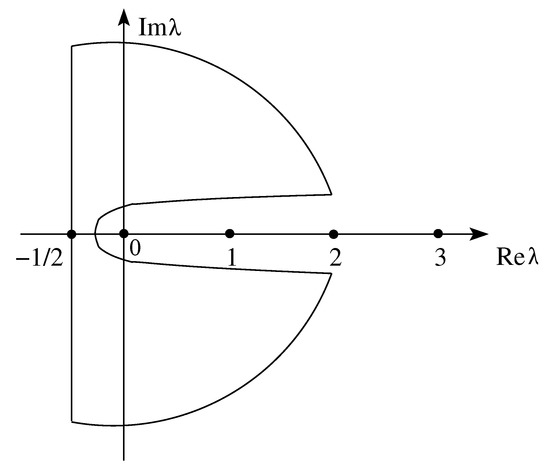
Exploiting the asymptotic behaviour of the Euler gamma function, integral (79) can be evaluated by the contour integration method along the path shown in Figure 4. Note that the poles of the gamma function $\Gamma (1/2-\mathrm{i}\nu )$ are located at $\nu =-\mathrm{i}(\ell +1/2)$, and allow us to pick up correctly the input data. In fact, we have: ${\left[\tilde{f}(-1/2+\mathrm{i}\nu )\right]}_{(\nu =-\mathrm{i}(\ell +1/2\left)\right)}=\tilde{f}(\ell )=f_{\ell }$. We obtain:

$$d_k=2\sqrt{\pi }\sum _{\ell =0}^{\infty }\frac{{(-1)}^{\ell }}{\ell !}{f}_{\ell }{\mathcal{P}}_k\left[-\mathrm{i}\left(\ell +\frac{1}{2}\right)\right].$$

(80)

Figure 4. Integration path used for evaluating integral (79) (see Lemma 1).

Next, we observe that:

$$\Gamma \left(\frac{1}{2}+\mathrm{i}\nu \right)={\int }_{-\infty }^{+\infty }{e}^{-\mathrm{i}\nu w}{e}^{{-e}^{-w}}{e}^{-w/2}\mathrm{d}w=\mathcal{F}\left\{e^{{-e}^{-w}}{e}^{-w/2}\right\},$$

(81)

where $\mathcal{F}$ denotes the Fourier integral operator. Let us note that the function $exp(-exp(-w\left)\right)exp(-w/2)$ belongs to the Schwartz space S of the $C^{\infty }\left(\mathbb{R}\right)$ functions that decrease with all their derivatives for $\left|w\right|$ tending to $+\infty$, faster than any negative power of $\left|w\right|$. Therefore we can write:

$${\psi }_k\left(\nu \right)=\frac{1}{\sqrt{\pi }}\mathcal{F}\left\{{\mathcal{P}}_k\left(-\mathrm{i}\frac{\mathrm{d}}{\mathrm{d}w}\right)\left[e^{{-e}^{-w}}{e}^{-w/2}\right]\right\}.$$

(82)

Inserting representation (82) of the Pollaczek functions into expansion (78), we obtain:

$$\tilde{f}\left(-\frac{1}{2}+\mathrm{i}\nu \right)=\sum _{k=0}^{\infty }{d}_k\left\{\frac{1}{\sqrt{\pi }}\mathcal{F}\left[{\mathcal{P}}_k\left(-\mathrm{i}\frac{\mathrm{d}}{\mathrm{d}w}\right)\left[e^{{-e}^{-w}}{e}^{-w/2}\right]\right]\right\}.$$

(83)

Now, we apply the inverse operator ${\mathcal{F}}^{-1}$ to the r.h.s. of Formula (83) and exchange the integral operator ${\mathcal{F}}^{-1}$ with the sum, this operation being legitimate within the $L^2$-norm convergence. We obtain:

$$\begin{array}{cc}\hfill {\mathcal{F}}^{-1}& \sum _{k=0}^{\infty }{d}_k\left\{\frac{1}{\sqrt{\pi }}\mathcal{F}\left[{\mathcal{P}}_k\left(-\mathrm{i}\frac{\mathrm{d}}{\mathrm{d}w}\right)\left[e^{{-e}^{-w}}{e}^{-w/2}\right]\right]\right\}\hfill \\ & =\sum _{k=0}^{\infty }{d}_k\left\{\frac{1}{\sqrt{\pi }}{\mathcal{F}}^{-1}\mathcal{F}\left[{\mathcal{P}}_k\left(-\mathrm{i}\frac{\mathrm{d}}{\mathrm{d}w}\right)\left[e^{{-e}^{-w}}{e}^{-w/2}\right]\right]\right\}.\hfill \end{array}$$

(84)

Finally, recalling Formula (74), we obtain the following expansion for the function $\widehat{F}\left(w\right)exp(w/2)$:

$$\widehat{F}\left(w\right)e^{w/2}=\frac{1}{\sqrt{\pi }}\sum _{k=0}^{\infty }{d}_k{\mathcal{P}}_k\left(-\mathrm{i}\frac{\mathrm{d}}{\mathrm{d}w}\right)\left[e^{{-e}^{-w}}{e}^{-w/2}\right],$$

(85)

the convergence being in the $L^2$-norm. It can be easily verified that:

$$\sqrt{2}{\mathcal{P}}_k\left(-\mathrm{i}\frac{\mathrm{d}}{\mathrm{d}w}\right)\left[e^{{-e}^{-w}}{e}^{-w/2}\right]={\mathrm{i}}^k\sqrt{2}{L}_k\left(2e^{-w}\right)e^{{-e}^{-w}}{e}^{-w/2},$$

(86)

where $L_k$ denotes the Laguerre polynomials [19].

It can be readily checked that the polynomials ${\mathcal{L}}_k\left(w\right)\doteq {\mathrm{i}}^k\sqrt{2}{L}_k\left(2e^{-w}\right)$ are a set of polynomials orthonormal on the real line with weight function $W\left(w\right)=exp(-w)exp(-2exp(-w\left)\right)$. Consequently, the set of functions ${\Phi }_k\left(w\right)$, defined by (73), represents an orthonormal basis in $L^2(-\infty ,+\infty )$.

Finally, from Formula (85) we obtain:

$$\widehat{F}\left(w\right)e^{w/2}=\sum _{k=0}^{\infty }{c}_k\left[{\mathrm{i}}^k\sqrt{2}{L}_k\left(2e^{-w}\right)e^{{-e}^{-w}}{e}^{-w/2}\right]=\sum _{k=0}^{\infty }{c}_k{\Phi }_k\left(w\right)(w\in {\mathbb{R}}^{+}),$$

(87)

where $c_k=d_k/\sqrt{2\pi }$, and the functions ${\Phi }_k\left(w\right)$ are given by (73). □

The successive step of the inversion procedure consists in inverting the Abel transform. Consider Formula (A42) and put: $coshv=y$, $coshw=x$. The Abel transform can be written as a convolution product of the following form:

$$\left(\mathcal{A}F\right)\left(x\right)=\sqrt{2}{\int }_1^x\frac{\underline{F}\left(y\right)}{\sqrt{(x-y)}}\mathrm{d}y\doteq \sqrt{2}(\underline{F}*{\chi }_1)\left(x\right).$$

(88)

From (53), we analogously obtain:

$$\underline{F}\left(y\right)=\frac{1}{\pi \sqrt{2}}\frac{\mathrm{d}}{\mathrm{d}y}{\int }_1^y\frac{\left(\mathcal{A}F\right)\left(x\right)}{\sqrt{(y-x)}}\mathrm{d}x\doteq \frac{1}{\pi \sqrt{2}}(\mathcal{A}F*{\chi }_1)\left(y\right).$$

(89)

We can now prove the following Lemma (see also [8]).

Lemma 2.

If the sequence $a_{\ell }={(\ell +1)}^p{f}_{\ell }$$(\ell \in {\mathbb{N}}_0)$ satisfies the Hausdorff condition (5) with $p⩾2$, then the following limit holds:

$$\underset{m\to \infty }{lim}⟨(\underline{F}-{\psi }_m),\varphi ⟩=0,$$

(90)

where

$${\psi }_m\left(y\right)=\frac{1}{\pi \sqrt{2}}\frac{\mathrm{d}}{\mathrm{d}y}\left[\left(\sum _{k=0}^m{c}_k{\Phi }_k\right)*{\chi }_1\right],$$

(91)

and $\varphi \in S_{\infty }\left(\mathbb{R}\right)$ ($S_{\infty }\left(\mathbb{R}\right)$ is the Schwartz space of the $C^{\infty }\left(\mathbb{R}\right)$ functions $\varphi \left(x\right)$ that, along with all their derivatives, decrease for $\left|x\right|\to \infty$ faster than any negative power of $\left|x\right|$), and $⟨f,\varphi ⟩$ denotes the Lebesgue integral ${\int }_{-\infty }^{\infty }\overline{f}\varphi \mathrm{d}x$.

Proof. 

From (89) and (91) we have:

$$\begin{array}{cc}\hfill ⟨(\underline{F}-{\psi }_m),\varphi ⟩& =\frac{1}{\pi \sqrt{2}}⟨\frac{\mathrm{d}}{\mathrm{d}y}\left[\left(\mathcal{A}F-\sum _{k=0}^m{c}_k{\Phi }_k\right)*{\chi }_1\right],\varphi ⟩\hfill \\ & =-\frac{1}{\pi \sqrt{2}}⟨\left(\mathcal{A}F-\sum _{k=0}^m{c}_k{\Phi }_k\right)*{\chi }_1,{\varphi }^{\prime }⟩(\varphi \in S_{\infty }\left(\mathbb{R}\right)).\hfill \end{array}$$

(92)

From inequality (28) and Formula (A42) it follows that $\mathcal{A}F$ has a power-like behaviour in x. Next, for the Fubini theorem, we have:

$$⟨\left(\mathcal{A}F-\sum _{k=0}^m{c}_k{\Phi }_k\right)*{\chi }_1,{\varphi }^{\prime }⟩=⟨\mathcal{A}F-\sum _{k=0}^m{c}_k{\Phi }_k,{\varphi }^{\prime }*{\chi }^{\infty }⟩,$$

(93)

where

$$({\varphi }^{\prime }*{\chi }^{\infty })\left(x\right)\doteq {\int }_x^{+\infty }\frac{{\varphi }^{\prime }\left(y\right)}{\sqrt{(y-x)}}\mathrm{d}y<\infty .$$

(94)

Next, from Schwarz’s inequality it follows:

$$⟨\mathcal{A}F-\sum _{k=0}^m{c}_k{\Phi }_k,{\varphi }^{\prime }*{\chi }^{\infty }⟩⩽{∥\mathcal{A}F-\sum _{k=0}^m{c}_k{\Phi }_k∥}_{L^2[0,+\infty )}·{∥{\varphi }^{\prime }*{\chi }^{\infty }∥}_{L^2[0,+\infty )}.$$

(95)

Now, since ${lim}_{m\to \infty }{∥\mathcal{A}F-{\sum }_{k=0}^m{c}_k{\Phi }_k∥}_{L^2[0,+\infty )}=0$ (see Lemma 1) and ${∥{\varphi }^{\prime }*{\chi }^{\infty }∥}_{L^2[0,+\infty )}<\infty$, statement (90) follows. □

Remarks 1.

(i) As mentioned at the end of Section 3, if only a subset of partial-waves ${\left\{f_l\right\}}_{{\ell }_0}^{\infty }$ satisfy condition (49), then $\tilde{f}\left(\lambda \right)$ is analytic only in the half-plane $\mathrm{Re}\lambda >{\ell }_0-\frac{1}{2}$. However, even in this case, the above inversion procedure can be applied with only minor technical modifications.

(ii) So far, we have assumed that all the partial-waves $f_{\ell }$ are known and, in addition, that are noiseless. A much more realistic analysis accounts that only a finite number of partial-waves ${\left\{f_{\ell }\right\}}_{\ell ={\ell }_0}^{{\ell }_1}$ can actually be known and that they are inevitably affected by noise. In this case, the reconstruction of $\widehat{F}\left(w\right)$ from this set of noisy data meets the difficulties related to the ill-posedness of the inverse problems. See Ref. [5] for a more detailed discussion of the algorithm of reconstruction from a finite set of noisy input data.

6. Born Approximation as a Laplace–Abel Transformation

Let us now consider the Born approximation. The partial-waves $f_{\ell }$, at the first-order Born approximation, are given (suitablly normalized) by

$$f_{\ell }\left(k\right)={\int }_0^{+\infty }{j}_{\ell }^2\left(kr\right)V_{{\mu }_0}\left(r\right)r^{2}dr,$$

(96)

where $j_{\ell }\left(kr\right)$ are the spherical Bessel functions of order ℓ. Then, exploiting the following formula:

$${\int }_0^{+\infty }{e}^{-\mu r}{J}_{\ell }^2\left(kr\right)dr=\frac{1}{\pi k}{Q}_{\ell -1/2}\left(1+\frac{{\mu }^2}{2k^2}\right),$$

(97)

recalling that $j_{\ell }\left(kr\right)=\sqrt{\pi /2kr}{J}_{\ell +1/2}\left(kr\right)$ and observing that $V_{{\mu }_0}\left(r\right)$ belongs to the Yukawian class (see representation (2)), we obtain:

$$f_{\ell }\left(k\right)=\frac{1}{2k^2}{\int }_{{\mu }_0}^{+\infty }{Q}_{\ell }\left(1+\frac{{\mu }^2}{2k^2}\right)\sigma \left(\mu \right)d\mu .$$

(98)

We put $\mu =\sqrt{t}=k{\left[2(coshv-1)\right]}^{1/2}$ and since on the cut we have $\theta$ equals $iv$, then Formula (98) can be rewritten as

$$f_{\ell }=\frac{1}{2}{\int }_{1+{\mu }_0^2/2k^2}^{+\infty }{Q}_{\ell }(coshv)\frac{\sigma \left(\mu \right)}{\mu }\mathrm{d}(coshv)({\mu }_0=k{\left[2(cosh{v}_0-1)\right]}^{1/2}).$$

(99)

Therefore, we can see that the restriction of $\tilde{f}\left(\lambda \right)$ to $\ell \in {\mathbb{N}}_0$ coincides with the first-order Born approximation of the partial-waves, after the following identification (see also [2]):

$$\frac{\sigma \left(\mu \right)}{\mu }=2\underline{F}\left(1+\frac{{\mu }^2}{2k^2}\right).$$

(100)

Formula (100) allows us to recover the spectral density $\sigma \left(\mu \right)$ from the jump function $\underline{F}$, but only in the domain ${\mu }_0^2<t<4{\mu }_0^2$, that is, where $\underline{F}$ coincides with the jump function associated with the first-order Born approximation (see [2]). In fact, we can write an equation of the Lippman–Schwinger-type for the discontinuities $\Delta f\doteq \mathrm{i}{lim}_{\stackrel{ϵ\to 0}{ϵ>0}}[f(\mathrm{i}v+ϵ)-f(\mathrm{i}v-ϵ)]$:

$$\Delta f={(\Delta f)}_0+\Delta f\diamond {(\Delta f)}_0,$$

(101)

where ${(\Delta f)}_0$ represents the discontinuity function associated with the first-order Born approximation. The convolution product ${}^{\prime }{\diamond }^{\prime }$ has as cycle of integration the compact one-shaped region determined by the support properties of the involved jump function [20]. Equation (101) has been investigated by many authors (see, e.g., [2] and the references quoted therein). Here, we limit ourselves to consider the results which are worth in our case. Equation (101) can be formally solved through the following Neumann–Born series:

$$\Delta f=\sum _{k=0}^{\infty }{\left(\Delta f\right)}_0^{\diamond k},$$

(102)

where ${(\Delta f)}_0^{\diamond 0}={(\Delta f)}_0$, (${(\Delta f)}_0=\Delta f$ in the domain ${\mu }_0^2<t<4{\mu }_0^2$), and ${(\Delta f)}_0^{\diamond k}={(\Delta f)}_0^{k-1}\diamond {(\Delta f)}_0$. These convolution products form an algebra, named Volterra algebra, which has found particular relevance in the study of the Bethe–Salpeter equation (see [4,20]). The domains on which $\Delta f$ and ${(\Delta f)}_0$ are defined permit us to implement an iterative procedure that, in principle, can reconstruct the spectral density $\sigma \left(\mu \right)$ completely (see [2]). In fact, if the support of ${(\Delta f)}_0$ is given by the values $t>{\mu }_0^2$, then the support of ${(\Delta f)}_0\diamond {(\Delta f)}_0$ will be $t>4{\mu }_0^2$. Therefore, within the interval $4{\mu }_0^2<t<9{\mu }_0^2$, the spectral density $\sigma \left(\mu \right)$ is

$$\frac{1}{2}\frac{\sigma \left(\mu \right)}{\mu }=\Delta f-{(\Delta f)}_0\diamond {(\Delta f)}_0(4{\mu }_0^2<t<9{\mu }_0^2).$$

(103)

This procedure can be iterated: for instance, for values of t in $9{\mu }_0^2<t<16{\mu }_0^2$ it involves a double convolution product. We have earlier shown that $\Delta f$ and ${(\Delta f)}_0$ enjoy a power-like behavior in $\mu$, but the entire iterative procedure is not guaranteed to maintain this type of behavior. Therefore, the existence of $V_{{\mu }_0}\left(r\right)$ cannot be proved rigorously. In other words, the behavior in $\mu$ of each multiple convolution product can be controlled, but when the amplitudes are restricted to be on the energy-shell, all the possible combination of the factors must be taken into consideration. This leads to an alternating series, whose global $\mu$-behavior cannot be controlled.

Summarizing, we can prove the existence of a spectral density $\sigma \left(\mu \right)$ which possesses a good local behavior and, in addition, we can reconstruct this function from the amplitudes by using an iterative procedure. Unfortunately, to date we are not able to keep under control the global $\mu$-behavior of the entire iterative procedure so to have guaranteed the convergence of integral (2) and, consequently, the existence of the potential $V_{{\mu }_0}\left(r\right)$.

7. Conclusions

We have shown that if the partial-waves $f_{\ell }$ of the Fourier–Legendre expansion of the scattering amplitude satisfy a suitable Hausdorff condition and are exponentially bounded, then this expansion converges to an analytic function $f\left(\theta \right)$, which can be holomorphically extended to a slit domain in the $cos\theta$-plane. The geometrical tool adopted to reach this result consists essentially in connecting the analysis on the complex $cos\theta$-plane with that on a complex hyperboloid $X^{\left(c\right)}$, which contains as submanifolds the support of the $SO(3,\mathbb{R})$ harmonic analysis and the support of the cut. Through a suitable fibration, obtained by a Radon-type transformation, we can limit ourselves to study the harmonic analysis on a one dimensional complex hyperbola, thus allowing us to regard the Fourier–Legendre series as a trigonometrical series. The holomorphic extension of the latter can then be translated back to the slit $cos\theta$-plane by inverting the Radon-type transform. The jump function describing the discontinuity on the cut is found to be related to the Laplace–Radon tranform of the analytic function interpolating uniquely the partial-waves $f_{\ell }$. The inversion of this transformation finally yields the spectral density $\sigma \left(\mu \right)$ and, under some additional restrictions, the potential $V_{{\mu }_0}\left(r\right)$. The key ingredient to achieve this result is the Haudorff condition (5) we imposed on the partial-waves. Such a condition, which firstly emerged in the theory of moments, calls for the analysis of the broader class of completely monotonic potentials which, in turn, find application in various problems, e.g., of extremal geometry. These issues will be the object of future investigations.

References

- Chadan, K.; Sabatier, P.C. Inverse Problems in Quantum Scattering Theory; Springer: New York, NY, USA, 1977. [Google Scholar]
- Martin, A.; Targonski, G.Y. On the Uniqueness of a Potential Fitting a Scattering Amplitude at a Given Energy. Nuovo Cimento 1961, 20, 1182–1190. [Google Scholar] [CrossRef][Green Version]
- Walsh, J.L. Approximation by Polynomials in the Complex Domain; Memorial des Sciences Matematique, Gauthier-Villars: Paris, France, 1935. [Google Scholar]
- Fioravanti, R.; Viano, G.A. On the Solution of the Inverse Scattering Problem, at Fixed Energy, for the Class of Yukawian Potentials. J. Math. Phys. 1995, 36, 5310–5339. [Google Scholar] [CrossRef]
- De Micheli, E.; Viano, G.A. Hausdorff Moments, Hardy Spaces and Power Series. J. Math. Anal. Appl. 1999, 234, 265–286. [Google Scholar] [CrossRef][Green Version]
- Widder, D.V. The Laplace Transform; Princeton Univ. Press: Princeton, NJ, USA, 1972. [Google Scholar]
- Boas, R.P. Entire Functions; Academic Press: New York, NY, USA, 1954. [Google Scholar]
- De Micheli, E.; Viano, G.A. Holomorphic Extension Associated with Fourier-Legendre Expansions. J. Geom. Anal. 2002, 12, 355–374. [Google Scholar] [CrossRef][Green Version]
- Watanabe, T. A Probabilistic Method in Hausdorff Moment Problem and Laplace-Stieltjes Transform. J. Math. Soc. Jpn. 1960, 12, 192–206. [Google Scholar] [CrossRef]
- Hunt, G.A. Markoff Processes and Potentials I. Illinois J. Math. 1957, 1, 44–93. [Google Scholar]
- Hunt, G.A. Markoff Processes and Potentials II. Illinois J. Math. 1957, 1, 316–369. [Google Scholar] [CrossRef]
- De Micheli, E. On the Connection between Spherical Laplace Transform and Non-Euclidean Fourier Analysis. Mathematics 2020, 8, 287. [Google Scholar] [CrossRef]
- Watson, G.N. The Diffraction of Electric Waves by the Earth. Proc. R. Soc. Lond. 1918, 95, 83–103. [Google Scholar]
- Bros, J.; Viano, G.A. Connection between the Harmonic Analysis on the Sphere and the Harmonic Analysis on the One-sheeted Hyperboloid: An Analytic Continuation Viewpoint II. Forum Math. 1996, 8, 659–722. [Google Scholar]
- Bros, J.; Viano, G.A. Connection between the Harmonic Analysis on the Sphere and the Harmonic Analysis on the One-sheeted Hyperboloid: An Analytic Continuation Viewpoint I. Forum Math. 1996, 8, 621–658. [Google Scholar]
- Erdélyi, A. (Ed.) Higher Trascendental Functions. In Bateman Manuscript Project; McGraw-Hill: New York, NY, USA, 1953; Volume 2. [Google Scholar]
- Szegö, G. Orthogonal Polynomials; American Mathematical Society: Providence, RI, USA, 1959. [Google Scholar]
- Itzykson, C. Group Representation in a Continuous Basis: An Example. J. Math. Phys. 1969, 10, 767–769. [Google Scholar] [CrossRef]
- Koornwinder, T.H. Meixner-Pollaczek Polynomials and the Heisenberg Algebra. J. Math. Phys. 1989, 30, 767–769. [Google Scholar] [CrossRef]
- Faraut, J.; Viano, G.A. Volterra Algebra and the Bethe-Salpeter Equation. J. Math. Phys. 1986, 27, 840–848. [Google Scholar] [CrossRef]
Publisher’s Note: MDPI stays neutral with regard to jurisdictional claims in published maps and institutional affiliations. |
© 2021 by the author. Licensee MDPI, Basel, Switzerland. This article is an open access article distributed under the terms and conditions of the Creative Commons Attribution (CC BY) license (https://creativecommons.org/licenses/by/4.0/).