A General Optimal Iterative Scheme with Arbitrary Order of Convergence

Abstract

A general optimal iterative method, for approximating the solution of nonlinear equations, of $(n+1)$ steps with $2^{n+1}$ order of convergence is presented. Cases $n=0$ and $n=1$ correspond to Newton’s and Ostrowski’s schemes, respectively. The basins of attraction of the proposed schemes on different test functions are analyzed and compared with the corresponding to other known methods. The dynamical planes showing the different symmetries of the basins of attraction of new and known methods are presented. The performance of different methods on some test functions is shown.

1. Introduction

Nonlinear equations and systems appear in many problems in computer science and other disciplines when they are modeled mathematically. In general, these equations have no analytical solution and we must resort to iterative processes to approximate their solutions.

In the literature, methods or families of iterative schemes, designed from different procedures, have proliferated in recent years to approximate the simple or multiple roots $\alpha$ of a nonlinear equation $f(x)=0$, where $f:D\subseteq \mathbb{R}\to \mathbb{R}$ is a real function defined on an open interval D. In the books [1,2], we can find many of the iterative schemes published in recent years and classified from different points of view. With them, we can have an overview of the state of the art in the research area of iterative processes for solving nonlinear equations. Of course, each scheme has a different behavior. This behavior is characterized with efficiency and stability criteria provided by the tools of complex dynamics.

The efficiency of these schemes has been widely considered, usually based on the efficiency index presented by Ostrowski [3]. The expression of this index, $I=p^{1/d}$, involves the order of convergence of the method p and the number of functional evaluations in each iteration, d. The methods with higher convergence order are not necessarily the most efficient, as the complexity of the iterative expression also plays an important role. In [4], Kung and Traub established that the order of convergence of an iterative method without memory, which used n functional evaluations per iteration, is less than or equal to $2^{n-1}$. When an iterative scheme reaches this upper bound, it is said to be an optimal method. Many optimal schemes have been designed in the last years with different order of convergence (see, e.g., [5,6,7,8,9,10] and the references therein).

One of the more used iterative schemes is Newton’s method, thanks to its efficiency and simplicity,

$$x_{k+1}=x_k-\frac{f(x_k)}{f^{\prime }(x_k)},k=0,1,2,\dots$$

(1)

Under certain conditions, this method has quadratic convergence and it is optimal.

It is known that Newton’s method can be combined with itself an arbitrary times $n+1$, obtaining a new scheme of order $2^{n+1}$, $n=1,2,3,\dots$ (see [11]).

$$\left\{\begin{array}{c}{y}_1=x_k-\frac{f(x_k)}{f^{\prime }(x_k)},\hfill \\ y_2=y_1-\frac{f(y_1)}{f^{\prime }(y_1)},\hfill \\ ⋮\hfill \\ y_{j+1}=y_j-\frac{f(y_j)}{f^{\prime }(y_j)},j=2,\dots ,n-2\hfill \\ ⋮\hfill \\ y_n=y_{n-1}-\frac{f(y_{n-1})}{f^{\prime }(y_{n-1})},\hfill \\ x_{k+1}=y_n-\frac{f(y_n)}{f^{\prime }(y_n)},\hfill \end{array}\right.$$

(2)

for $k=0,1,2,\dots$. This method is not optimal following the Kung–Traub conjecture [4]. We modify expression (2) to obtain an optimal iterative scheme of order $2^{n+1}$. To do this, we approximate the derivatives appearing in (2) after the first step by polynomials satisfying certain conditions.

In the remainder of this paper, we discuss the following points. In Section 2, the iterative expression of the proposed schemes is obtained, while its order of convergence is proven in Section 3. Section 4 is devoted to analyzing the dynamical planes of the proposed methods and other known ones when they are applied to different nonlinear equations. The numerical results are described in Section 5. With some conclusions and the references used in this manuscript, we finish the paper.

2. Design of the Class of Iterative Procedures

Now, we design the proposed family and prove its converge. From expression (2) and approximating the derivative after the first step, we obtain the following iterative expression:

$$\left\{\begin{array}{c}{y}_1=x_k-\frac{f(x_k)}{f^{\prime }(x_k)},\hfill \\ y_2=y_1-\frac{f(y_1)}{P_2^{\prime }(y_1)},\hfill \\ ⋮\hfill \\ y_{n-1}=y_{n-2}-\frac{f(y_{n-2})}{P_{n-1}^{\prime }(y_{n-2})},\hfill \\ y_n=y_{n-1}-\frac{f(y_{n-1})}{P_n^{\prime }(y_{n-1})},\hfill \\ x_{k+1}=y_n-\frac{f(y_n)}{P_{n+1}^{\prime }(y_n)},\hfill \end{array}\right.$$

(3)

where $y_0=x_k$ and $P_j(x)={\displaystyle {\displaystyle \sum _{i=0}^j}}{a}_i{(x-y_{j-1})}^i$, for $j=2,\dots ,n+1$, and polynomials $P_j(x)$ satisfy

• $P_j(y_i)=f(y_i)$ for $i=0,\dots ,j-1$.
• $P_j^{\prime }(y_0)=f^{\prime }(y_0)$.

Now, we obtain an explicit expression for $P_j^{\prime }(y_{j-1})$, $j=2,3,\dots ,n+1$, which we use in each step. To simplify the expression, we take $j=n+1$. Thus,

$$P_{n+1}(x)=a_{n+1}{(x-y_n)}^{n+1}+a_{n-1}{(x-y_n)}^{n-1}+\dots +a_1(x-y_n)+a_0.$$

From the conditions that polynomial must be satisfied, it is easy to observe that $P_{n+1}(y_n)=a_0=f(y_n)$ and that we need the expression of $a_1$ since $P_{n+1}^{\prime }(y_n)=a_1$. Thus, we need to solve

$$\left(\begin{array}{ccccc}{(y_{n-1}-y_n)}^{n+1}& {(y_{n-1}-y_n)}^n& \dots & (y_{n-1}-y_n)& 1\\ {(y_{n-2}-y_n)}^{n+1}& {(y_{n-2}-y_n)}^n& \dots & (y_{n-2}-y_n)& 1\\ ⋮& ⋮& & ⋮& ⋮\\ {(y_0-y_n)}^{n+1}& {(y_0-y_n)}^n& \dots & (y_0-y_n)& 1\\ (n+1){(y_0-y_n)}^n& n{(y_0-y_n)}^{n-1}& \dots & 1& 0\end{array}\right)\left(\begin{array}{c}{a}_{n+1}\\ a_n\\ ⋮\\ a_2\\ a_1\\ a_0\end{array}\right)=\left(\begin{array}{c}f(y_{n-1})\\ f(y_{n-2})\\ ⋮\\ f(y_0)\\ f^{\prime }(y_0)\end{array}\right),$$

which is equivalent to

$$\left(\begin{array}{ccccc}{(y_{n-1}-y_n)}^n& {(y_{n-1}-y_n)}^{n-1}& \dots & (y_{n-1}-y_n)& 1\\ {(y_{n-2}-y_n)}^n& {(y_{n-2}-y_n)}^{n-1}& \dots & (y_{n-2}-y_n)& 1\\ ⋮& ⋮& & ⋮& ⋮\\ {(y_0-y_n)}^n& {(y_0-y_n)}^{n-1}& \dots & (y_0-y_n)& 1\\ (n+1){(y_0-y_n)}^n& n{(y_0-y_n)}^{n-1}& \dots & 2(y_0-y_n)& 1\end{array}\right)\left(\begin{array}{c}{a}_{n+1}\\ a_n\\ ⋮\\ a_2\\ a_1\end{array}\right)=\left(\begin{array}{c}f[y_{n-1},y_n]\\ f[y_{n-2},y_n]\\ ⋮\\ f[y_0,y_n]\\ f^{\prime }(y_0)\end{array}\right),$$

where $f[y_j,y_n]$ are the divided differences of $y_j$ and $y_n$ in f, that is, $f[y_j,y_n]=\frac{f(y_j)-f(y_n)}{y_j-y_n}$.

By using algebraic operations between the two last rows, we obtain

$$\left(\begin{array}{ccccc}{(y_{n-1}-y_n)}^n& {(y_{n-1}-y_n)}^{n-1}& \dots & (y_{n-1}-y_n)& 1\\ {(y_{n-2}-y_n)}^n& {(y_{n-2}-y_n)}^{n-1}& \dots & (y_{n-2}-y_n)& 1\\ ⋮& ⋮& & ⋮& ⋮\\ {(y_0-y_n)}^n& {(y_0-y_n)}^{n-1}& \dots & (y_0-y_n)& 1\\ n{(y_0-y_n)}^{n-1}& (n-1){(y_0-y_n)}^{n-2}& \dots & 1& 0\end{array}\right)\left(\begin{array}{c}{a}_{n+1}\\ a_n\\ ⋮\\ a_2\\ a_1\end{array}\right)=\left(\begin{array}{c}f[y_{n-1},y_n]\\ f[y_{n-2},y_n]\\ ⋮\\ f[y_0,y_n]\\ \frac{f^{\prime }(y_0)-f[y_0,y_n]}{(y_0-y_n)}\end{array}\right).$$

Then, the coefficient matrix of the system is a Vandermonde confluent matrix; thus, it is invertible, and the system can be solved.

Let us see how a system with Vandermonde confluent matrix is solved, which can be found in more detail in [12,13]. For solving the previous system, we denote by $b_i=y_i-y_n$, $i=0,1,\dots ,n-1$, define $P(x)={(x-b_0)}^2(x-b_1)\dots (x-b_{n-1})$ and the Vandermonde confluent matrix

$$V=\left(\begin{array}{ccccc}1& 0& 1& \dots & 1\\ b_0& 1& b_1& \dots & b_{n-1}\\ b_0^2& 2b_0& b_1^2& \dots & b_{n-1}^2\\ ⋮& ⋮& ⋮& & ⋮\\ b_0^n& n{b}_0^{n-1}& b_1^n& \dots & b_{n-1}^n\end{array}\right).$$

Let $P_j(x)=\frac{P(x)}{{(x-b_j)}^{m_j}}$ be a polynomial, where $m_j$ is the maximum exponent of $x-b_j$, that is,

$$P_0(x)=\frac{P(x)}{{(x-b_0)}^2}={\displaystyle \prod _{i=1}^{n-1}}(x-b_i),$$

$$P_j(x)=(x-b_0){\displaystyle \prod _{i=0,i\ne j}^{n-1}}(x-b_i),\forall j\ne 0.$$

We define $g_j(x)=\frac{1}{P_j(x)}$ and

$$L_{j,k_j}(x)=P_j(x){(x-b_j)}^{k_j}{\displaystyle \sum _{i=0}^{m_j-k_j-1}}\frac{1}{i!}{g}_j^{(i)}(b_j){(x-b_j)}^i,0\le k_j\le m_j-1.$$

Then, we have

$$V^{-1}=\left(\begin{array}{cccc}{L}_{0,0}(0)& L_{0,0}^{\prime }(0)& \dots & \frac{1}{(n-1)!}{L}_{0,0}^{(n-1)}(0)\\ L_{0,1}(0)& L_{0,1}^{\prime }(0)& \dots & \frac{1}{(n-1)!}{L}_{0,1}^{(n-1)}(0)\\ L_{1,0}(0)& L_{1,0}^{\prime }(0)& \dots & \frac{1}{(n-1)!}{L}_{1,0}^{(n-1)}(0)\\ ⋮& ⋮& & ⋮\\ L_{n-1,0}(0)& L_{n-1,0}^{\prime }(0)& \dots & \frac{1}{(n-1)!}{L}_{n-1,0}^{(n-1)}(0)\end{array}\right).$$

Since $V^T$ is involved in our system, we use the transpose of $V^{-1}$ to obtain the values of parameters $a_i$.

Thus, in our case, we need the first component of the following matrix product:

$$\left(\begin{array}{ccccc}{L}_{0,0}(0)& L_{0,1}(0)& L_{1,0}(0)& \dots & L_{n-1,0}(0)\\ L_{0,0}^{\prime }(0)& L_{0,1}^{\prime }(0)& L_{1,0}^{\prime }(0)& \dots & L_{n-1,0}^{\prime }(0)\\ ⋮& ⋮& ⋮& & ⋮\\ \frac{1}{(n-1)!}{L}_{0,0}^{(n-1)}(0)& \frac{1}{(n-1)!}{L}_{0,1}^{(n-1)}(0)& \frac{1}{(n-1)!}{L}_{1,0}^{(n-1)}(0)& \dots & \frac{1}{(n-1)!}{L}_{n-1,0}^{(n-1)}(0)\end{array}\right)\left(\begin{array}{c}f[y_0,y_n]\\ \frac{f^{\prime }(y_0)-f[y_0,y_n]}{(y_0-y_n)}\\ f[y_1,y_n]\\ ⋮\\ f[y_{n-1},y_n]\end{array}\right).$$

It follows that

$$a_1=L_{0,1}(0)\frac{f^{\prime }(y_0)-f[y_0,y_n]}{(y_0-y_n)}+{\displaystyle \sum _{j=0}^{n-1}}{L}_{j,0}(0)f[y_j,y_n].$$

We now determine $L_{0,1}(0)$ and $L_{j,0}(0)$ for $j=0,\dots ,n-1$. We have,

$$g_0(x)=\frac{1}{{\prod }_{i=1}^{n-1}(x-b_i)},$$

$$g_0^{\prime }(x)=-\frac{1}{{\prod }_{i=1}^{n-1}(x-b_i)}{\displaystyle \sum _{i=1}^{n-1}}\frac{1}{(x-b_i)},$$

$$g_j(x)=\frac{1}{(x-b_0){\prod }_{i=0,i\ne j}^{n-1}(x-b_i)}.$$

Therefore, the expressions of $L_{0,0}(0)$, $L_{0,1}(x)$ and $L_{j,0}$ when $j\ne 0$, are

$$L_{0,0}(0)={(-1)}^{n-1}{\displaystyle \prod _{i=1}^{n-1}}\frac{b_i}{b_0-b_i}\left(1+b_0{\displaystyle \sum _{i=1}^{n-1}}\frac{1}{(b_0-b_i)}\right),$$

$$L_{0,1}(0)={(-1)}^n{b}_0{\displaystyle \prod _{i=1}^{n-1}}\frac{b_i}{(b_0-b_i)},$$

$$L_{j,0}(0)={(-1)}^n\frac{b_0}{(b_j-b_0)}{\displaystyle \prod _{i=0,i\ne j}^{n-1}}\frac{(b_i)}{(b_j-b_i)}.$$

Thus, by grouping the terms properly, we get that $a_1$ has the form

$$\begin{array}{cc}\hfill a_1=& {(-1)}^n{\displaystyle \prod _{i=1}^{n-1}}\frac{b_i}{b_0-b_i}\left(f^{\prime }(y_0)-\left(2+{\displaystyle \sum _{i=1}^{n-1}}\frac{b_0}{b_0-b_i}\right)f[y_0,y_n]\right)\hfill \\ \hfill & +{(-1)}^n{\displaystyle \sum _{j=1}^{n-1}}\frac{b_0}{b_j-b_0}{\displaystyle \prod _{i=0,i\ne j}^{n-1}}\frac{b_i}{b_j-b_i}f[y_j,y_n].\hfill \end{array}$$

Thus, we get the form of the term $a_1$ in each step.

Some of the members of this class are as follows.

The two-step method has the iterative expression

$$\left\{\begin{array}{c}{y}_1=x_k-\frac{f(x_k)}{f^{\prime }(x_k)},\hfill \\ x_{k+1}=y_1-\frac{f(y_1)}{2f[x_0,x_1]-f^{\prime }(x_0)},\hfill \end{array}\right.$$

(4)

This is the Ostrowski’s method, with order of convergence four. We denote by $M4$ scheme (4).

Let us now look at the three-step method:

$$\left\{\begin{array}{c}{y}_1=x_k-\frac{f(x_k)}{f^{\prime }(x_k)},\hfill \\ y_2=y_1-\frac{f(y_1)}{2f[x_0,x_1]-f^{\prime }(x_0)},\hfill \\ x_{k+1}=y_2-\frac{f(y_2)}{a_1},\hfill \end{array}\right.$$

(5)

where

$$a_1=\frac{f[y_1,y_2]{(x_k-y_2)}^2+(y_1-y_2)(f^{\prime }(x_k)(x_k-y_1)+f[x_k,y_2](-3x_k+2y_1+y_2))}{{(x_k-y_1)}^2},$$

whose order of convergence is 8. We denote method (5) by $M8$.

Let us remark that the extension of this family for solving nonlinear systems is not straightforward, except in the first step, as it involves vectorial interpolation polynomials.

3. Convergence Analysis

Let $f:D\subset \mathbb{R}\to \mathbb{R}$ be a sufficiently differentiable function in an open interval D that contains a zero $\alpha$ of f. We consider the divided difference operator

$$f[x+h,x]={\int }_0^1{f}^{\prime }(x+th)dt,$$

(6)

as defined by Genochi-Hermite [14]. By using Taylor’s expression of $f^{\prime }(x+th)$ around x, we obtain

$$f[x+h,x]=f^{\prime }(x)+\frac{1}{2}{f}^{\prime \prime }(x)h+\frac{1}{6}{f}^{\prime \prime \prime }(x)h^2+O(h^3),$$

(7)

which we employ to prove the following theorem, where the order of convergence of the method defined in (3) is established.

Theorem 1.

Let $f:D\subset \mathbb{R}⟶\mathbb{R}$ be a sufficiently differentiable function in a neighbourhood D of α, such that $f(\alpha )=0$ and $f^{\prime }(\alpha )\ne 0$. Then, choosing an initial estimation $x_0$ close to α, sequence $\left\{x_k\right\}$ generated by the $(n+1)$-step method (3) converge to α with order of convergence $2^{n+1}$.

Proof. 

We prove this result by induction on the number of steps. The one-step method defined in (3) is the Newton’s scheme, so we know that the one-step method has order of convergence 2. Now, we assume that the i-step method has order of convergence $2^i$ where $i\le j$. Thus, we prove that the $j+1$-step method has order $2^{j+1}$.

We denote that $y_0=x_0$ and $y_i$ is defined in (3). First, we calculate the expression of the polynomial $P_{j+1}$.

$$P_{j+1}(x)=P_j(x)+(f(y_j)-P_j(y_j))\left({\displaystyle \prod _{i=0}^{j-1}}\frac{x-y_i}{y_j-y_i}\right)\frac{x-x_0}{y_j-x_0}.$$

Moreover,

$$f(x)-P_{j+1}(x)=\frac{f^{(j+2)}(ϵ)}{(j+2)!}(x-y_j)\cdots (x-y_1){(x-x_0)}^2,$$

where $ϵ$ is a point in the interpolation interval. Thus, we know that

$$f^{\prime }(x)-P_{j+1}^{\prime }(x)=\frac{f^{(j+2)}(ϵ)}{(j+2)!}\left((x-x_0)\left({\displaystyle \sum _{r=0}^j}{\displaystyle \prod _{i=0,i\ne r}^j}(x-y_i)\right)+2{\displaystyle \prod _{i=0}^j}(x-y_i)\right).$$

Evaluating the last expression in $y_j$, we have

$$f^{\prime }(y_j)-P_{j+1}^{\prime }(y_j)=\frac{f^{(j+2)}(\alpha )}{(j+2)!}(y_j-x_0){\displaystyle \prod _{i=0}^{j-1}}(y_j-y_i).$$

Defining $C_i=\frac{1}{i!}\frac{f^{(i)}(\alpha )}{f^{\prime }(\alpha )}$, we obtain

$$P_{j+1}^{\prime }(y_j)=f^{\prime }(y_j)-C_{j+2}{f}^{\prime }(\alpha )(y_j-x_0){\displaystyle \prod _{i=0}^{j-1}}(y_j-y_i).$$

Using the Taylor’s expression of $f(y_i)$ around $\alpha$:

$$f(y_i)=f^{\prime }(\alpha )\left(y_i-\alpha +C_2{(y_i-\alpha )}^2+O({(y_i-\alpha )}^3)\right).$$

(8)

Then, $f^{\prime }(y_i)$ around $\alpha$ has the following expression:

$$\begin{array}{cc}\hfill f^{\prime }(y_i)& =f^{\prime }(\alpha )\left(1+2C_2(y_i-\alpha )\right)+O({(y_i-\alpha )}^2).\hfill \end{array}$$

(9)

Using the last part of the expression of $P_{j+1}$, we deduce that

$$P_{j+1}^{\prime }(y_j)=f^{\prime }(\alpha )\left(1+2C_2(y_j-\alpha )\right)+O({(y_j-\alpha )}^2)-C_{j+2}{f}^{\prime }(\alpha )(y_j-x_0){\displaystyle \prod _{i=0}^{j-1}}(y_j-y_i).$$

We assume that the i-step method has order of convergence $2^i$ for $i\le j$, that is, $y_i-\alpha =M_i{(x_0-\alpha )}^{2^i}+O({(x_0-\alpha )}^{2^i+1})$. Taking $e=x_0-\alpha$, we obtain

$$y_i-\alpha =M_i{e}^{2^i}+O(e^{2^i+1}).$$

Now, we calculate ${\displaystyle \prod _{i=0}^{j-1}}(y_j-y_i)$. We have that

$$y_j-y_i=(y_j-\alpha )-(y_i-\alpha )=M_j{e}^{2^j}-M_i{e}^{2^i}+O(e^{2^i+1})=-M_i{e}^{2^i}+O(e^{2^i+1}).$$

From the above expression, we obtain

$$\begin{array}{cc}\hfill {\displaystyle \prod _{i=0}^{j-1}}(y_j-y_i)& ={\displaystyle \prod _{i=0}^{j-1}}(-M_i{e}^{2^i}+O(e^{2^i+1}))\hfill \end{array}$$

(10)

$$\begin{array}{cc}& =({\displaystyle \prod _{i=0}^{j-1}}-M_i)e^{{\displaystyle \sum _{i=0}^{j-1}}{2}^i}+O(e^{{\displaystyle \sum _{i=0}^{j-1}}{2}^i+1}))\hfill \end{array}$$

(11)

$$\begin{array}{cc}& ={(-1)}^j{e}^{2^j-1}{\displaystyle \prod _{i=0}^{j-1}}{M}_i+O(e^{2^j})).\hfill \end{array}$$

(12)

Then,

$$\begin{array}{cc}\hfill P_{j+1}^{\prime }(y_j)=& f^{\prime }(\alpha )\left(1+2C_2(y_j-\alpha )\right)+O({(y_j-\alpha )}^2)\hfill \\ & -C_{j+2}{f}^{\prime }(\alpha )(y_j-x_0)({(-1)}^j{e}^{2^j-1}{\displaystyle \prod _{i=0}^{j-1}}{M}_i+O(e^{2^j})).\hfill \end{array}$$

As $y_j-x_0=-e+O(e^2)$ and $y_j-\alpha =M_j{e}^{2^j}+O(e^{2^j+1})$ is satisfied,

$$\begin{array}{cc}\hfill P_{j+1}^{\prime }(y_j)& =f^{\prime }(\alpha )\left(1+2C_2{M}_j{e}^{2^j}\right)-C_{j+2}{f}^{\prime }(\alpha )({(-1)}^{j+1}{e}^{2^j}{\displaystyle \prod _{i=0}^{j-1}}{M}_i)+O(e^{2^j+1})\hfill \end{array}$$

(13)

$$\begin{array}{c}=f^{\prime }(\alpha )\left(1+e^{2^j}(2C_2{M}_j+C_{j+2}{(-1)}^j{\displaystyle \prod _{i=0}^{j-1}}{M}_i)\right)+O(e^{2^j+1}).\hfill \end{array}$$

(14)

We need to calculate now the expression of $\frac{f(y_j)}{P_{j+1}^{\prime }(y_j)}$.

$$\begin{array}{cc}\hfill \frac{f(y_j)}{P_{j+1}^{\prime }(y_j)}& =\frac{\left(y_j-\alpha +C_2{(y_j-\alpha )}^2+O({(y_j-\alpha )}^3)\right)}{\left(1+e^{2^j}(2C_2{M}_j+C_{j+2}{(-1)}^j{\displaystyle {\displaystyle \prod _{i=0}^{j-1}}}{M}_i)\right)+O(e^{2^j+1})}\hfill \end{array}$$

(15)

$$\begin{array}{c}=\frac{(y_j-\alpha )+C_2{M}_j^2{e}^{2^{j+1}}+O(e^{2^{j+1}+1})}{1+e^{2^j}(2C_2{M}_j+C_{j+2}{(-1)}^j{\displaystyle {\displaystyle \prod _{i=0}^{j-1}}}{M}_i)+O(e^{2^j+1})}.\hfill \end{array}$$

(16)

Thus,

$$\begin{array}{cc}\hfill y_{j+1}-\alpha & =y_j-\alpha -\frac{f(y_j)}{P_{j+1}^{\prime }(y_j)}\hfill \\ & =y_j-\alpha -\frac{(y_j-\alpha )+C_2{M}_j^2{e}^{2^{j+1}}+O(e^{2^{j+1}+1})}{1+e^{2^j}(2C_2{M}_j+C_{j+2}{(-1)}^j{\displaystyle {\displaystyle \prod _{i=0}^{j-1}}}{M}_i)+O(e^{2^j+1})}\hfill \\ & =\frac{(y_j-\alpha )\left(e^{2^j}(2C_2{M}_j+C_{j+2}{(-1)}^j{\displaystyle {\displaystyle \prod _{i=0}^{j-1}}}{M}_i)+O(e^{2^j+1})\right)-C_2{M}_j^2{e}^{2^{j+1}}+O(e^{2^{j+1}+1})}{1+e^{2^j}(2C_2{M}_j+C_{j+2}{(-1)}^j{\displaystyle {\displaystyle \prod _{i=0}^{j-1}}}{M}_i)+O(e^{2^j+1})}\hfill \\ & =\frac{\left(e^{2^{j+1}}(2C_2{M}_j^2+C_{j+2}{(-1)}^j{\displaystyle {\displaystyle \prod _{i=0}^j}}{M}_i)\right)-C_2{M}_j^2{e}^{2^{j+1}}+O(e^{2^{j+1}+1})}{1+e^{2^j}(2C_2{M}_j+C_{j+2}{(-1)}^j{\displaystyle {\displaystyle \prod _{i=0}^{j-1}}}{M}_i)+O(e^{2^j+1})}\hfill \\ & =\frac{e^{2^{j+1}}(C_2{M}_j^2+C_{j+2}{(-1)}^j{\displaystyle {\displaystyle \prod _{i=0}^j}}{M}_i)+O(e^{2^{j+1}+1})}{1+e^{2^j}(2C_2{M}_j+C_{j+2}{(-1)}^j{\displaystyle {\displaystyle \prod _{i=0}^{j-1}}}{M}_i)+O(e^{2^j+1})}.\hfill \end{array}$$

From the last expression, we obtain

$$y_{j+1}-\alpha =e^{2^{j+1}}(C_2{M}_j^2+C_{j+2}{(-1)}^j{\displaystyle {\displaystyle \prod _{i=0}^j}}{M}_i)+O(e^{2^{j+1}+1}).$$

Thus, we prove that the $j+1$-step method (3) has order of convergence $2^{j+1}$; thus, by induction, the $n+1$-step method has order of convergence $2^{n+1}$. □

In this case, our $n+1$-step method carries out $n+2$ evaluations, since we carry out the derivative of f in $x_0$ and also the image of f in the approximations $x_0,y_1,\dots ,y_n$. For this reason, we have that the proposed family of methods (3) is optimal according to the conjecture of Kung and Traub, because $2^{n+1}=2^{n+2-1}$.

4. Complex Dynamics

The order of convergence is not the only criterion that must be analyzed in an iterative scheme. The relevance of the method also depends on how it behaves according to the initial estimations, so it is necessary to analyze the dynamics of the method, that is, the dynamics of the rational operator obtained when the scheme is applied on polynomials with low degree.

The dynamical study of a family of iterative methods allows classifying them, based on their behavior with respect to the initial approximations taken, into stable methods and chaotic ones. This analysis also provides important information on the reliability of the methods [15,16,17,18,19].

In this section, we focus on studying the complex dynamics of the methods M4, defined in (4), and M8, defined in (5), members of the proposed family (3). Now, we remember some concepts of complex dynamics. These contents can be enlarged by viewing different classical books (see, e.g., [20]).

Given a rational function $R:\widehat{\mathbb{C}}\to \widehat{\mathbb{C}}$, where $\widehat{\mathbb{C}}$ is the Riemann sphere, the orbit of a point $z_0\in \widehat{\mathbb{C}}$ is defined as:

$$\{z_0,R\left(z_0\right),R^2\left(z_0\right),...,R^n\left(z_0\right),...\}.$$

A $z_0\in \widehat{\mathbb{C}}$ is called a fixed point if $R\left(z_0\right)=z_0$. For the proposed methods, the roots of the polynomial are fixed points, but there may be other fixed points, different from the roots, which we call strange fixed points. A critical point $z_0$ is a point such that $R^{\prime }\left(z_0\right)=0$, and it is called free critical point when it is different from the roots of $f(x)$. The stability of a fixed point $z_0$ depends on the value of the derivative $R^{\prime }$ in it. In fact, it is called attractor if $|R^{\prime }(z_0)|<1$, superattractor if $|R^{\prime }(z_0)|=0$, repulsor if $|R^{\prime }(z_0)|>1$ and parabolic if $|R^{\prime }(z_0)|=1$.

The basin of attraction of an attractor $\alpha$ is defined as the set of points whose orbit tends to $\alpha$:

$$\mathcal{A}\left(\alpha \right)=\{z_0\in \widehat{\mathbb{C}}:R^n\left(z_0\right)\to \alpha ,n\to \infty \}.$$

Theorem 2.

(Cayley Quadratic Test (CQT)).

Let $Op(z)$ be the rational operator obtained from a general iteration formula applied to the quadratic polynomial $q(z)=(z-{\alpha }_1)(z-{\alpha }_2)$, with ${\alpha }_1\ne {\alpha }_2$. Suppose that $Op(z)$ is conjugate to the operator $z\to z^p$, by the Möbius transformation $M(z)=\frac{z-{\alpha }_1}{z-{\alpha }_2}$. Then, p is the order of the iterative method associated to $Op(z)$. Moreover, the corresponding Julia set $J(Op(z))$ is the circumference of center zero and radius 1.

Methods $M4$ and $M8$ verify the Cayley quadratic test, that is, the associated operator to each of them can be transformed by Möbius transformation into the operator $z^p$, being p the order of the method, so it follows that they are stable methods, where the only superattractors fixed points are the roots of the quadratic polynomial, the strange fixed points are repulsors and there are no free critical points.

In addition, when the Cayley quadratic test is satisfied, the Julia set of these methods on a quadratic polynomial is the circumference of center zero and unit radius.

Now, we construct the dynamical planes of methods $M4$ and $M8$ on other equations, and we compare them with those obtained with other known schemes of order 4 and 8. We compare the proposed schemes with Newton’s method, since we generate our methods from it. The two methods of order 4 used in the comparison are Jarratt’s scheme, which can be found in [21], whose iterative expression is

$$\left\{\begin{array}{c}{y}_1=x_k-\frac{2}{3}\frac{f(x_k)}{f^{\prime }(x_k)},\hfill \\ x_{k+1}=y_1-\frac{1}{2}\frac{f(x_k)}{f^{\prime }(x_k)}\frac{3f^{\prime }(y_1)+f^{\prime }(x_k)}{3f^{\prime }(y_1)-f^{\prime }(x_k)},\hfill \end{array}\right.$$

(17)

and the King’s family method, with $\beta =1$, which can be found in [22],

$$\left\{\begin{array}{c}{y}_1=x_k-\frac{f(x_k)}{f^{\prime }(x_k)},\hfill \\ x_{k+1}=y_1-\frac{f(y_1)}{f^{\prime }(x_k)}\frac{f(x_k)+f(y_1)}{f(x_k)-f(y_1)},\hfill \end{array}\right.$$

(18)

Method (17) is denoted by $J4$ and method (18) by $K4$.

On the other hand, methods of order 8 used in the comparison are the method denoted by $J8$, defined in [23], whose expression is

$$\left\{\begin{array}{c}{y}_1=x_k-\frac{f(x_k)}{f^{\prime }(x_k)},\hfill \\ \eta =x_k-\frac{1}{8}\frac{f(x_k)}{f^{\prime }(x_k)}-\frac{3}{8}\frac{f(x_k)}{f^{\prime }(y_1)},\hfill \\ y_2=x_k-6\frac{f(x_k)}{f^{\prime }(x_k)+f^{\prime }(y_1)+4f^{\prime }(\eta )},\hfill \\ x_{k+1}=y_2-\frac{f(y_2)}{f^{\prime }(x_k)}\frac{f^{\prime }(x_k)+f^{\prime }(y_1)-f^{\prime }(\eta )}{2f^{\prime }(y_1)-f^{\prime }(\eta )},\hfill \end{array}\right.$$

(19)

and the method denoted by $K8$, defined in [24], which is defined as

$$\left\{\begin{array}{c}{y}_1=x_k-\frac{f(x_k)}{f^{\prime }(x_k)},\hfill \\ y_2=y_1-\frac{f(y_1)}{f^{\prime }(x_k)}\frac{f(x_k)+f(y_1)}{f(x_k)-f(y_1)},\hfill \\ x_{k+1}=y_2-\frac{H_3(y_2)}{f^{\prime }(y_2)},\hfill \end{array}\right.$$

(20)

where

$$\begin{array}{cc}\hfill H_3(y_2)=& f(x_k)+f^{\prime }(x_k)\frac{{(y_2-y_1)}^2(y_2-x_k)}{(y_1-x_k)(x_k+2y_1-3y_2)}+f^{\prime }(y_2)\frac{(y_2-y_1)(x_k-y_2)}{(x_k+2y_1-3y_2)}\hfill \\ \hfill & -f[x_k,y_1]\frac{{(y_2-x_k)}^3}{(y_1-x_k)(x_k+2y_1-3y_2)},\hfill \end{array}$$

which, as we can see in [24], is obtained from King’s family schemes.

We apply all these methods on the following equations, which are also the equations that we use in the numerical experiments.

• $cos(x)-x=0$;
• ${(x-1)}^6-1=0$;
• $arctan(x)=0$; and
• $arctan(x)-\frac{2x}{x^2+1}=0$.

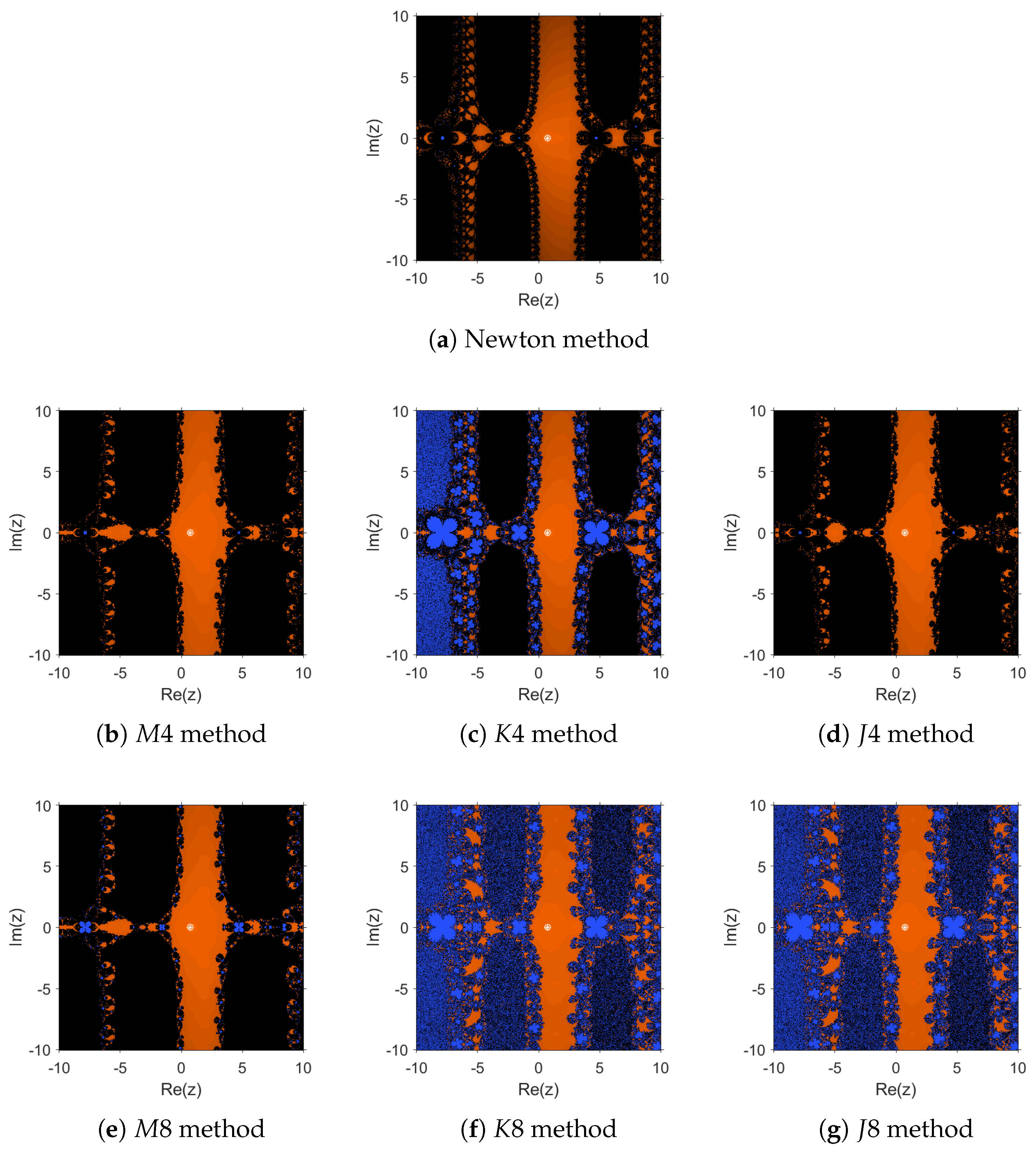
We select a region of the complex plane and establish a mesh. Each point of the mesh is considered as an initial approximation for the iterative method and painted in a certain color depending on where it converges to. For the dynamic planes, we choose a mesh of $400\times 400$ points and a maximum number of 40 iterations per point. Fixed points are represented by white circles while superattractors are represented by stars. All dynamical planes show different kinds of symmetries, with independence of the number of attracting fixed points of the related operator.

We can examine the dynamic planes associated with the different methods mentioned above for the equation $cos(x)-x=0$ in Figure 1. In this case, the points of the plane that converge to the approximate solution 0.73908513 are colored orange; the points that tend to infinity are colored blue, which we determine as the points whose value of the iteration in absolute value is greater than 800; and the points that do not converge are colored black. The dynamic planes that have a more complex structure are those associated with the $K4$ and $K8$ methods, in Figure 1c,f, while those corresponding to the rest of the methods present fewer intersections between the different basins.

Figure 1. Dynamical planes of $cos(x)-x=0$ for the new and known methods: (a) Newton, (b) M4 (4), (c) K4 (18), (d) J4 (18), (e) M8 (5), (f) K8 (20) and (g) J8 (19).

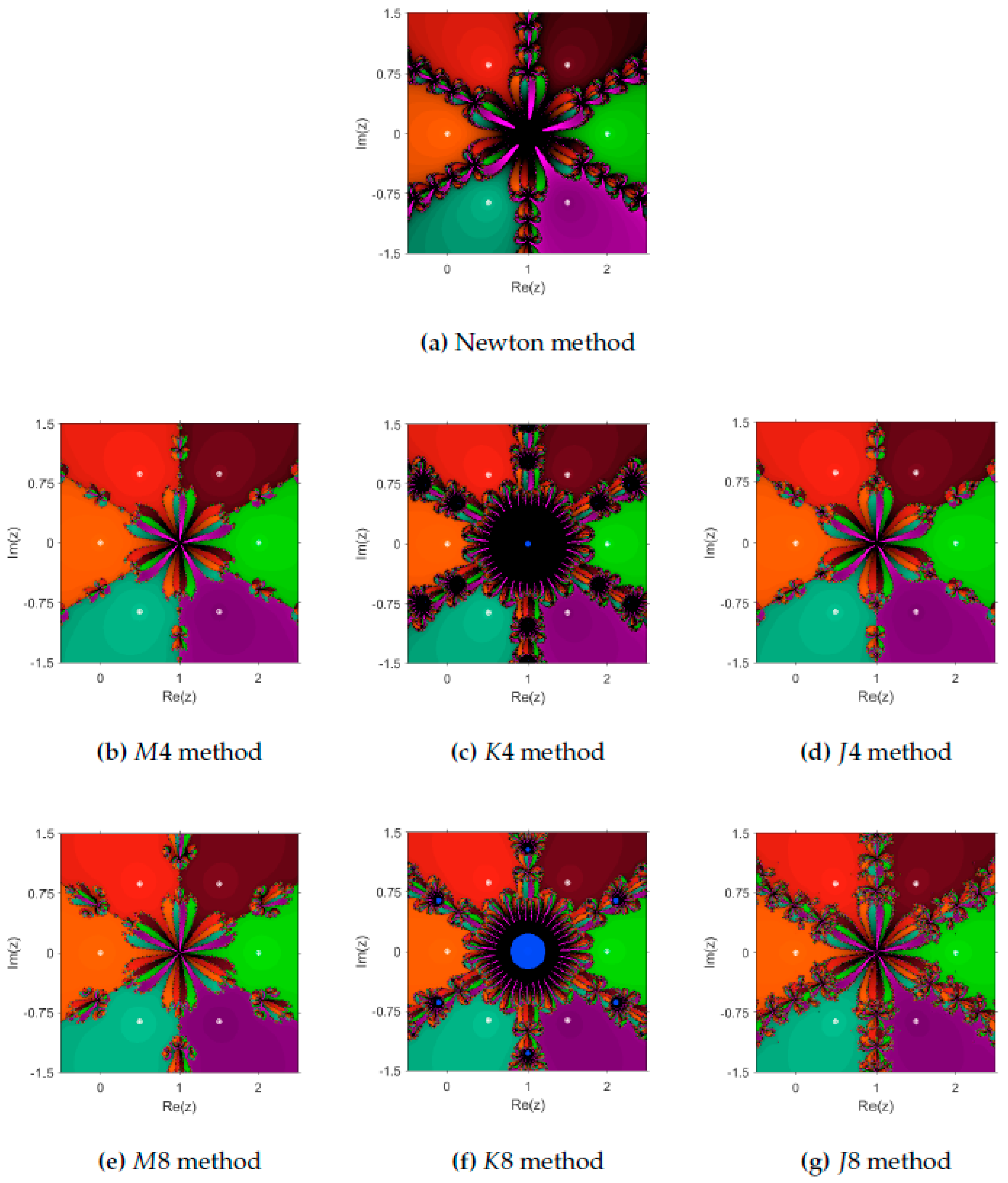
Let us now see what happens in the case of the equation ${(x-1)}^6-1=0$, whose dynamical planes are shown in Figure 2. In this case, there are more noticeable changes between the different dynamic planes, although in all cases we have the same superattractor fixed points, to which we associate each of the colors represented in the planes, except for black, which is associated with the initial points that do not converge to any superattractor fixed point, and blue, which is associated with the initial estimates whose iterations, in absolute value, are greater than 800.

Figure 2. Dynamical planes of ${(x-1)}^6-1=0$ for the new and known methods: (a) Newton, (b) M4 (4), (c) K4 (18), (d) J4 (18), (e) M8 (5), (f) K8 (20) and (g) J8 (19).

In this case, it can be seen that the planes that stand out most for their non-convergence zones in the center are those associated to the methods $K4$ and $K8$, as shown in Figure 2c,f; for this reason, these methods would not be recommended for initial estimations that are in that zone. On the other hand, we can see that Newton’s method has a larger black area than the Jarratt type methods or the methods proposed in the paper. If we analyze the dynamic planes associated to $M4$ and $J4$, we can see that it is a little simpler in the case of $M4$ method, but, if we compare the $M8$ and $J8$ methods, the dynamic plane is considerably simpler in the case of $M8$ scheme. For this equation, we do not study the strange fixed points, since we need to solve polynomials of high degree. As a conclusion, from these figures, it is highlighted that the most stable method for this example is $M8$ scheme.

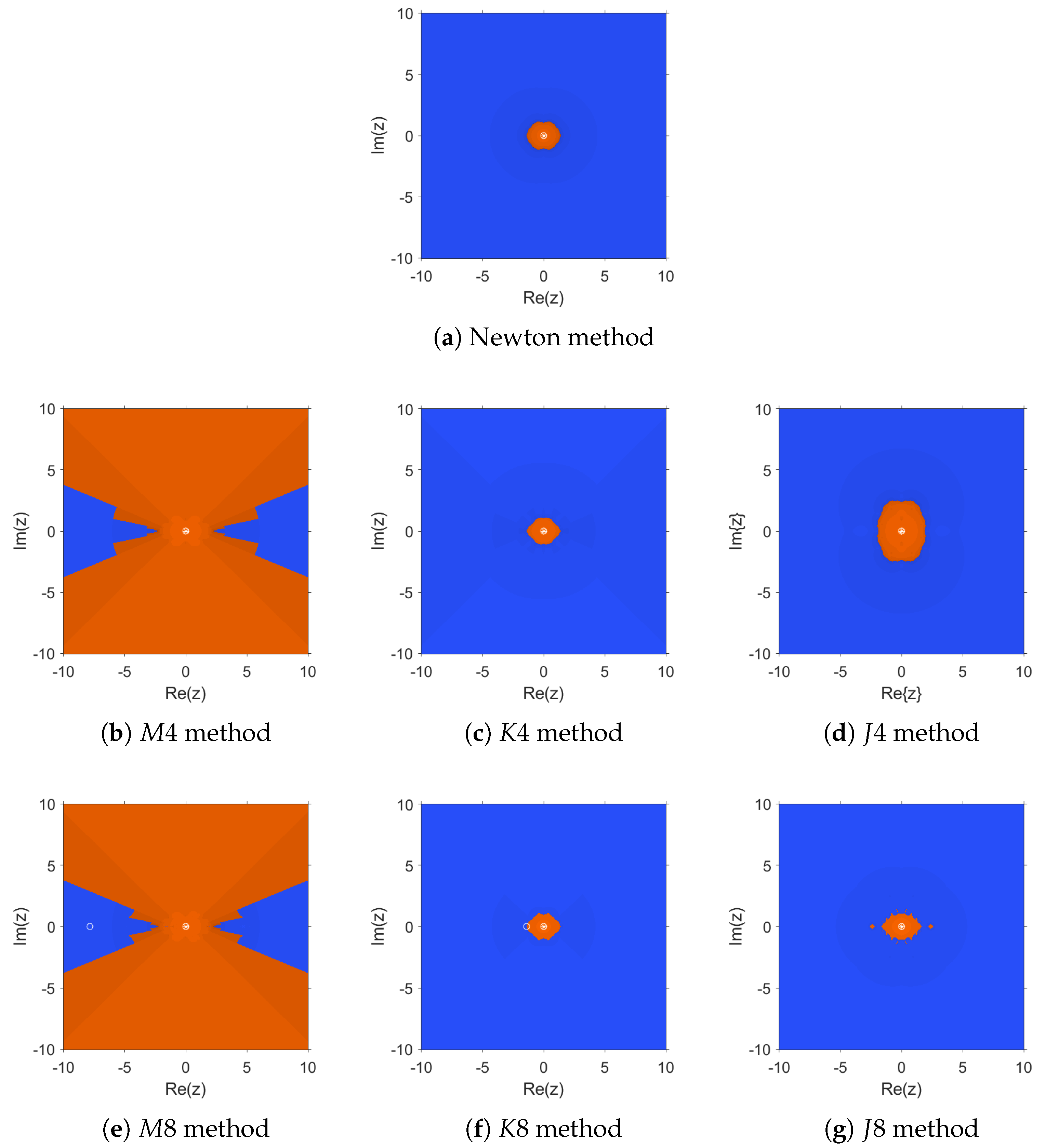
Let us now analyze the dynamical planes associated with the equation $arctanx=0$, which is shown in Figure 3. In this case, the initial estimations converging to the solution 0 are in orange and those converging to ∞ are in blue, which are determined as the initial estimates whose iterations, in absolute value, are greater than 800. We note that most of the planes are similar, except those associated with methods $M4$ and $M8$, since they have a basin of attraction for the 0 point much larger than in the rest of the cases, being a little greater that of method $M4$; for this reason, it is more convenient in this case to take one of these two methods since we have a greater number of initial estimations that converge to the solution that we are looking for.

Figure 3. Dynamical planes of $arctan(x)=0$ for the new and known methods: (a) Newton, (b) M4 (4), (c) K4 (18), (d) J4 (18), (e) M8 (5), (f) K8 (20) and (g) J8 (19).

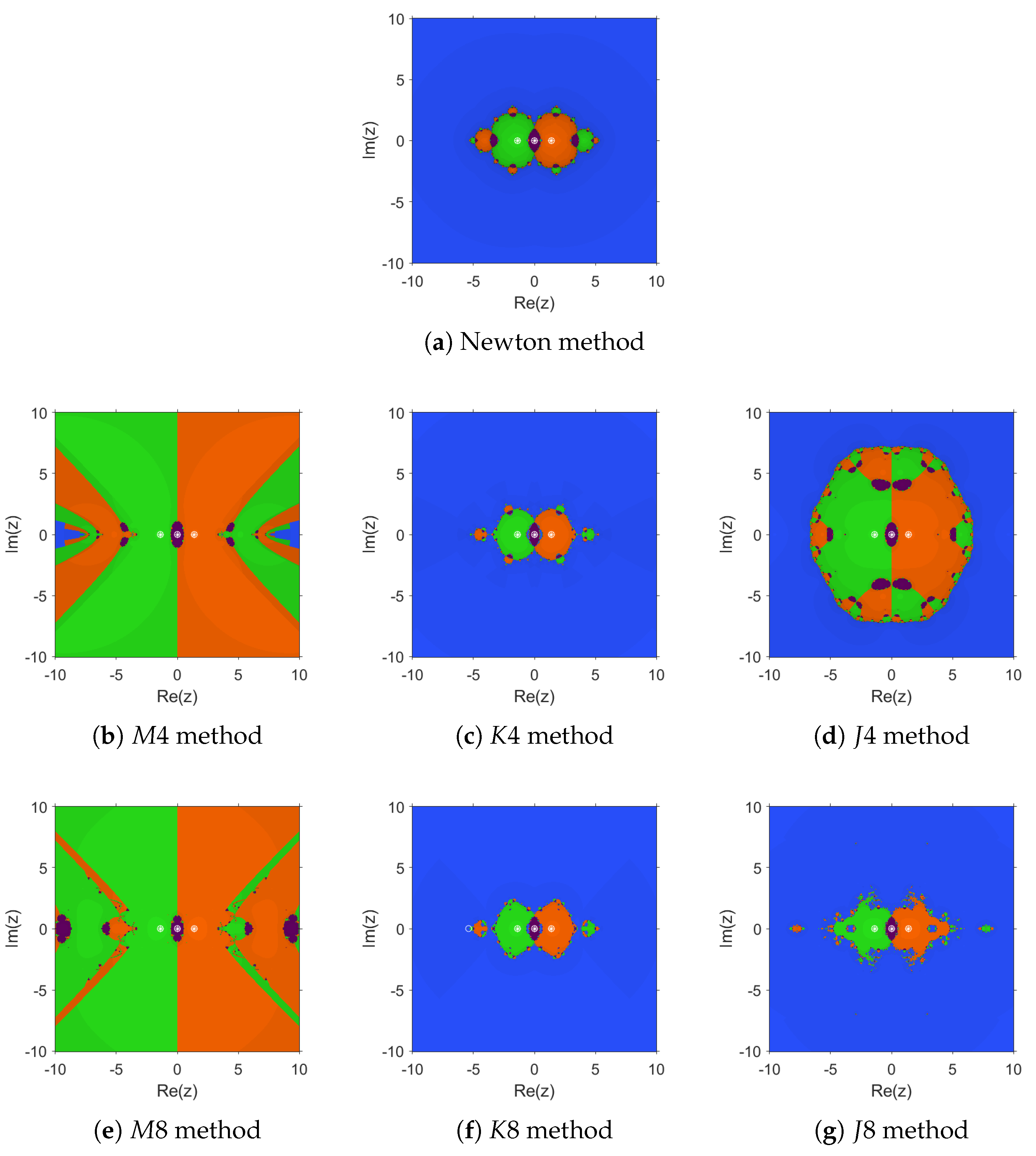
Let us now look at the dynamic planes associated with the equation $arctan(x)-\frac{2x}{x^2+1}=0$ in Figure 4. In this case, we illustrate in purple the initial estimates that converge to the solution $x=0$, in green the initial estimates that converge to the solution $x\approx -1.3917$, in orange those that converge to the solution $x\approx 1.3917$ and in blue the initial estimates that converge to $x\approx 1.3917$, which are determined as the initial estimates whose iteration in absolute value is greater than 800.

Figure 4. Dynamical planes of $arctan(x)-\frac{2x}{x^2+1}=0$ for the new and known methods: (a) Newton, (b) M4 (4), (c) K4 (18), (d) J4 (18), (e) M8 (5), (f) K8 (20) and (g) J8 (19).

In this example, we observe that most of the planes are similar, except for those associated with methods $M4$, $J4$ and $M8$, but among these three we can see that the one with the largest convergence area to ∞ is method $J4$, so it would be less convenient to use this method. If we look at the dynamic planes associated with the $M4$ and $M8$ methods, we can see that they are similar, although we emphasize the $M8$ method a little more as it has a smaller blue region.

After commenting on the dynamic planes of these cases, what we see is that, in general, for these examples, the methods that have given good results and have been the most convenient are the $M4$ and $M8$ methods, since they have a larger basin of attraction in the cases we are interested in, they do not generate other basins of attraction from strange fixed points and their dynamic planes are not as complex as the others in general.

5. Numerical Experiments

In this section, we solve some nonlinear equations to compare our proposed methods with other schemes of the same order of convergence to confirm the information obtained in the previous section.

For the computational calculations, we used Matlab R2020b, with arithmetic precision variable of 1000 digits, iterating from an initial estimate $x_0$ and with the stopping criterium $|f(x_{k+1})|<{10}^{-100}$ and $|x_{k+1}-x_k|<{10}^{-100}$.

In the different tables we show, for each test function and iterative scheme, the approximation of the root, the value of the function in the last iteration, the number of iterations required, the distance between the last two iterations, the computational time in seconds and the approximate computational convergence order (ACOC), defined in [25], the expression of which is

$$p\approx ACOC=\frac{ln(|x_{k+1}-x_k|/|x_k-x_{k-1}|)}{ln(|x_k-x_{k-1}|/|x_{k-1}-x_{k-2}|)}.$$

We work with the same methods used in the previous section and with equations:

• Equation $cos(x)-x=0$, which has an approximate solution at $x\approx 0.73908513$, and we take as the initial estimate for all methods $x_0=1$.
• Equation ${(x-1)}^6-1=0$, which has a solution at $x=2$, and we take as the initial estimate for all methods $x_0=1.5$.
• Equation $arctan(x)=0$, which has a solution at $x=0$, and we take as the initial estimate for all methods $x_0=1.5$.
• Equation $arctan(x)-\frac{2x}{x^2+1}=0$, which has a solution at $x=0$, and we take as the initial estimate for all methods $x_0=0.4$.

In Table 1, we show the results obtained for equation $cos(x)-x=0$. In this case, all methods converge to the solution, although there are differences between them. As expected, Newton’s method performs more iterations than the rest and thus also has a longer time. It also has the longest distance between the last two iterations.

Table 1. Results for the equation $cos(x)-x=0$.

Method	$\parallel \mathit{f}({\mathit{x}}_{\mathit{k}}){\parallel }_2$	$\parallel {\mathit{x}}_{\mathit{k}+1}-{\mathit{x}}_{\mathit{k}}{\parallel }_2$	Iteration	ACOC	Time
Newton	7.11815 $\times {10}^{-167}$	1.8724 $\times {10}^{-333}$	8	2	0.2856
$M4$	4.21403 $\times {10}^{-296}$	1.41767 $\times {10}^{-1008}$	5	4	0.1984
$K4$	1.90125 $\times {10}^{-279}$	1.41767 $\times {10}^{-1008}$	5	4	0.1922
$J4$	1.6318 $\times {10}^{-299}$	1.41767 $\times {10}^{-1008}$	5	4	0.1906
$M8$	5.27514 $\times {10}^{-640}$	1.41767 $\times {10}^{-1008}$	4	8	0.1875
$K8$	9.74433 $\times {10}^{-270}$	9.91668 $\times {10}^{-1008}$	4	6	0.1944
$J8$	6.51848 $\times {10}^{-608}$	1.41767 $\times {10}^{-1008}$	4	8	0.2031

Among the fourth-order methods, we can see that all the results are similar in terms of the number of iterations, the computational time and the value of the function at the last iteration.

If we now look at the results of the methods of order 8, we can see that they perform the same number of iterations, but in this case the $M8$ method has less computational time, followed by the $J8$ method, as happens in the case of the norm of the equation evaluated in the last iteration, i.e., in this case the $M8$ method gives us better results than the $J8$ method, and the latter better than the $K8$ method.

The conclusion of this numerical experiment is that all methods obtain similar results, although it would be advisable in this case to use the $M8$ method as it is the one that takes the least computational time, one of the fewest iterations and obtains the highest order, and it is by far the method that obtains the closest approximation to the solution, as can be seen in Columns 2 and 3 of Table 1.

The results obtained for the equation ${(x-1)}^6-1=0$ are shown in Table 2. In this case, not all the methods converge to the solution, since the methods $K4$ and $K8$ do not converge taking as initial estimate $x_0=1.5$, as can be seen in the dynamic planes associated with these methods for the equation ${(x-1)}^6-1=0$. This fact is denoted in the table as n.c.

Table 2. Results for the equation ${(x-1)}^6-1=0$.

Method	$\parallel \mathit{f}({\mathit{x}}_{\mathit{k}}){\parallel }_2$	$\parallel {\mathit{x}}_{\mathit{k}+1}-{\mathit{x}}_{\mathit{k}}{\parallel }_2$	Iteration	ACOC	Time
Newton	2.72448 $\times {10}^{-119}$	1.11342 $\times {10}^{-166}$	19	2	0.5164
$M4$	2.83553 $\times {10}^{-271}$	0	9	4	0.3250
$K4$	n.c.	n.c.	n.c.	n.c.	n.c.
$J4$	2.02789 $\times {10}^{-263}$	0	9	4	0.3328
$M8$	3.7096 $\times {10}^{-468}$	0	7	8	0.3281
$K8$	n.c.	n.c.	n.c.	n.c.	n.c.
$J8$	3.10018 $\times {10}^{-130}$	0	7	7.9992	0.3641

Let us now comment on the methods that do converge. In the previous case, Newton’s method was different from the rest of the methods, and in this case it is the same, although the difference between them is more notable since the number of iterations has grown considerably, as has the computational time. This is also the method that converges with the greatest distance between the last two iterations. Among the fourth-order methods, we can see that the results are similar in terms of number of iterations, computational time and the value of the function in the last iteration. If we now look at the eighth-order methods, we can see that the same number of iterations is performed, but in this case the $M8$ method has less computational time, although what stands out most from this table is that the norm of the equation evaluated in the last iteration of the $M8$ method is smaller than in the rest of the methods, and it is considerably smaller than in the case of the $J8$ method. As a conclusion of this numerical experiment, we obtain that among the converging methods we have similar results in most cases, although the $M8$ method stands out since it is one of those that makes fewer iterations and obtains a higher order, and it is by far the method that obtains a closer approximation to the solution, as can be seen in Column 2 and 3 of Table 2.

The results obtained for the equation $arctan(x)=0$ are presented in Table 3. In this case, not all the methods converge to the solution, since the Newton, $K4$ and $K8$ methods do not converge taking as initial estimation $x_0=1.5$, as can be seen in the dynamic planes associated to these methods for the equation $arctan(x)=0$. Let us discuss the methods that do converge. Among the fourth-order methods, we can see that the results of number of iterations, computational time and the value of the equation in the last iteration are similar. If we now look at the eighth-order methods, we can observe that the $M8$ method performs fewer iterations and also has the shortest computational time, although what stands out most in this table is the value of the ACOC of the $M8$ method, which in this case increases to 11 instead of 8, although it is true that the $J8$ method also increases to 9 and has the smallest value of the norm of the equation evaluated in the last iteration, although, by performing one more iteration than the $M8$ method, it is logical for this to happen.

Table 3. Results for the equation $arctan(x)=0$.

Method	$\parallel \mathit{f}({\mathit{x}}_{\mathit{k}}){\parallel }_2$	$\parallel {\mathit{x}}_{\mathit{k}+1}-{\mathit{x}}_{\mathit{k}}{\parallel }_2$	Iteration	ACOC	Time
Newton	n.c.	n.c.	n.c.	n.c.	n.c.
$M4$	2.55693 $\times {10}^{-252}$	2.42873 $\times {10}^{-1259}$	6	5	0.2250
$K4$	n.c.	n.c.	n.c.	n.c.	n.c.
$J4$	7.27099 $\times {10}^{-263}$	1.80085 $\times {10}^{-1270}$	6	5	0.2594
$M8$	5.654 $\times {10}^{-126}$	1.11859 $\times {10}^{-1379}$	4	10.9979	0.1891
$K8$	n.c.	n.c.	n.c.	n.c.	n.c.
$J8$	1.98863 $\times {10}^{-777}$	0	5	9	0.2672

As a conclusion of this numerical experiment, we obtain similar results among the converging methods, although the $M4$ and $M8$ methods stand out due to their dynamic planes, but especially the $M8$ method since it is the one that makes fewer iterations and obtains the highest order, besides being the one that takes the least time.

We show the results obtained for the equation $arctan(x)-\frac{2x}{x^2+1}=0$ in Table 4. In this case, all methods converge to the solution, as can be seen in the dynamic planes associated with these methods for the equation $arctan(x)-\frac{2x}{x^2+1}=0$.

Table 4. Results for the function $arctan(x)-\frac{2x}{x^2+1}$.

Method	$|\mathit{f}({\mathit{x}}^{(\mathit{k})})|$	$|{\mathit{x}}^{(\mathit{k}+1)}-{\mathit{x}}^{(\mathit{k})}|$	Iteration	ACOC	Time
Newton	2.63224 $\times {10}^{-843}$	9.24306 $\times {10}^{-282}$	14	3	0.5891
M4	1.67544 $\times {10}^{-2131}$	4.96455 $\times {10}^{-427}$	6	5	0.3359
K4	4.84918 $\times {10}^{-2200}$	9.73169 $\times {10}^{-441}$	11	5	0.6359
J4	2.27536 $\times {10}^{445}$	9.05734 $\times {10}^{-438}$	6	5	0.4297
M8	6.46592 $\times {10}^{-2102}$	1.33304 $\times {10}^{-219}$	4	11	0.2797
K8	3.25561 $\times {10}^{-1343}$	2.25726 $\times {10}^{-269}$	7	9	0.5328
J8	5.74708 $\times {10}^{-1218}$	4.84986 $\times {10}^{-136}$	4	9.00019	0.3141

Let us comment the methods as they appear in the table. As we can see, Newton’s method is the one that performs more iterations to reach the same tolerance, although it is true that for this example the ACOC increases by one unit.

If we look at the methods of order 4, we can see that in all of them the value of the ACOC is 5, when the expected value is 4. Among these methods, the one that performs the most iterations is the $K4$ method, and therefore the one that takes the longest. If we look at the $M4$ and $J4$ methods, the results are similar, although the $M4$ method gives a better approximation in this case with the same number of iterations, and also takes less time; thus, for this example, the most convenient method of order 4 would be the $M4$ method.

Regarding methods of order 8, we can see that $K8$ method performs more iterations than the rest of the schemes, as well as being one of the methods that uses the most computational time. We also observe that $M8$ method has the shortest computational time, although what stands out most in this table is the value of the ACOC of the $M8$ method, since in this case it increases to 11 instead of 8, although it is true that the $J8$ and $K8$ methods also increase to 9. In addition, $M8$ method obtains a more accurate approximation than the rest of the order 8 methods.

As a conclusion of this numerical experiment, we obtain that there are notable differences among the methods, highlighting as less convenient in this case the Newton and King type methods, and as more convenient methods we highlight for their results and dynamic planes the $M4$ and $M8$ methods, but especially the $M4$ method for its dynamic planes and the $M8$ method since it is the one that performs fewer iterations and obtains greater order, besides being the one that takes less time.

After performing these experiments, we can conclude that in these cases the most recommendable methods are $M4$ and $M8$ because they are the only methods, together with $J4$, that converge to the solution in all cases, and because they are the methods that stand out for their numerical results in all examples, although the one that stands out most from these two methods that we propose is the $M8$ method.

6. Conclusions

In this manuscript, we design a family of optimal iterative methods with $n+1$ steps and order of convergence $2^{n+1}$, for $n=0,1,2,\dots$.

From this class, we can select an optimal iterative scheme with the desired order of convergence. Some classical methods are members of this class.

We work, from the dynamic and numerical point of view, with the elements of this family of orders 4 and 8, comparing the results obtained with those of other known methods. The results provided by the two elements of the family are very satisfactory, both numerical (number of iterations, error bounds, etc.) and stability related (amplitude of the convergence basins, existence of strange fixed points, etc.).