Mixed Sensitivity-Based Robust H_∞ Control Method for Real-Time Hybrid Simulation

Abstract

Real-time hybrid simulation (RTHS), dividing the emulated structure into numerical substructures (NS) and physical substructures (PS), is a powerful technique to obtain responses and then to assess the seismic performance of civil engineering structures. A transfer system, a servo-hydraulic actuator or shaking table, is used to apply boundary conditions between the two substructures. However, the servo-hydraulic actuator is inherently a complex system with nonlinearities and may introduce time delays into the RTHS, which will decrease the accuracy and stability of the RTHS. Moreover, there are various uncertainties in RTHS. An accurate and robust actuator control strategy is necessary to guarantee reliable simulation results. Therefore, a mixed sensitivity-based H_∞ control method was proposed for RTHS. In H_∞ control, the dynamics and robustness of the closed-loop transfer system are realized by performance weighting functions. A form of weighting function was given considering the requirement in RTHS. The influence of the weighting functions on the dynamics was investigated. Numerical simulations and actual RTHSs were carried out under symmetric and asymmetric dynamic loads, namely sinusoidal and earthquake excitation, respectively. Results indicated that the H_∞ control method used for RTHS is feasible, and it exhibits an excellent tracking performance and robustness.

1. Introduction

Real-time hybrid simulation (RTHS) [1], or the real-time substructure pseudo-dynamic test, is a cost-effective and versatile experimental technique to evaluate structural performance under dynamic excitations. It originated from the pseudo-dynamic test [2] first proposed by a Japanese researcher in the 1970s, which is known as hybrid simulation (HS) nowadays. HS takes advantage of numerical analysis and physical experiments, in which the emulated structure is divided into several substructures: the part that cannot be simulated exactly is experimentally tested in the laboratory, which is denoted as the physical substructure (PS), and the rest is simulated by a computer program, which is denoted as the numerical substructure (NS) [3,4]. In RTHS, boundary conditions between the two substructures are imposed on the PS by a transfer system, a servo-hydraulic actuator or shaking table, in a real-time manner. This allows RTHS the ability to test rate-dependent components, such as TMD, AMD, and MR dampers. In recent decades, much progress has been achieved [5,6,7,8].

However, due to the inherent nonlinear dynamics of the actuator–specimen system, the desired displacement cannot be realized at the end of the time integration step. This is often called the time delay, which will decrease the accuracy and may lead to RTHS instabilities [9]. Therefore, to carry out a successful RTHS, the detrimental effect of time delay must be mitigated. Horiuchi et al. [9] assumed a constant time delay and proposed a polynomial extrapolation method. Subsequently, more accurate strategies have been investigated to consider the variation in time delay [10,11,12,13].

Modern control theory was also used to deal with time delay, where the control plant includes the servo-hydraulic and the specimen. The inverse control technique was introduced by Chen and Ricles [14], where the servo-hydraulic actuator is modeled by a first-order transfer function. Carrion and Spencer [15] proposed a model-based control approach, where a low-pass filter is combined with the inverted actuator system plant. In this method, a higher-order control plant can be used. Ning et al. [16] proposed an adaptive feedforward control method, where the Kalman filter is used to estimate the adjustable parameters. Xu et al. proposed a frequency evaluation index-based compensation for RTHS [17]. A two-stage delay compensation method, combining the feedforward and polynomial extrapolation, was proposed by Wang et al. [18]. A polynomial-based feedforward prediction algorithm was combined with a robust linear-quadratic-gaussian controller that was proposed by Zhou et al. [19] to deal with the adverse effects of time delay. Ning et al. [20] proposed an adaptive feedforward and feedback control method based on a discrete control plant, of which the model order is not restrained.

However, there are differences between the control plant model and the actuator–specimen system. Hence, preliminary discussions have been made on the robustness of the control strategy to model uncertainties [21,22,23]. In this study, a mixed sensitivity-based H_∞ control method was introduced to deal with the time delay and uncertainties in real-time hybrid simulation. The H_∞ control theory is overviewed in Section 2. The selection of a performance weighting function is presented in Section 3, where the influence of the weighting function on the system dynamics is discussed. Subsequently, the proposed method is validated through numerical simulations and actual RTHS in Section 4 and Section 5, respectively.

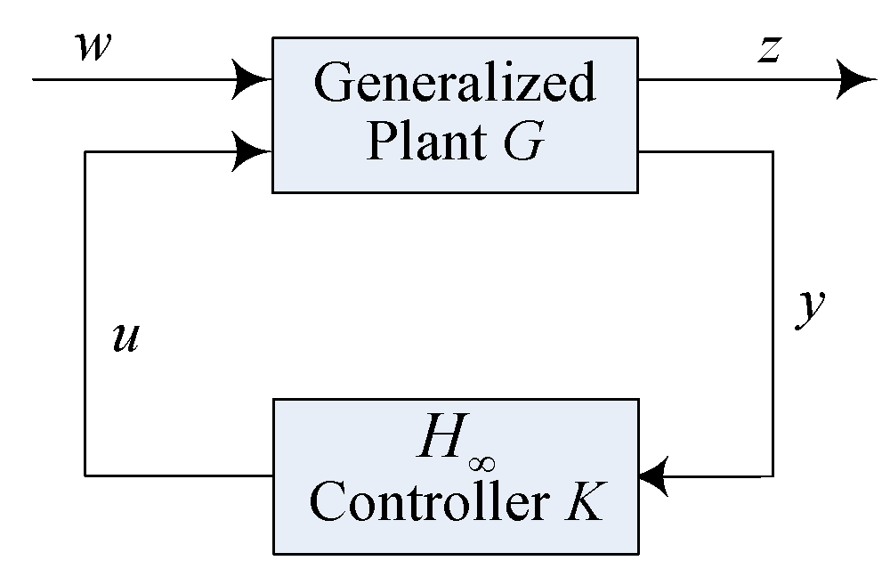
2. Overview of H_∞ Control Theory

The standard setup of H_∞ control is shown in Figure 1. In this figure, w, u, z, and y are vector-valued signals: w is the exogenous input, typically consisting of command signals, disturbances, and sensor noises; u is the control signal; z is the performance output that is to be minimized; y is the measured output. G is the generalized plant and K is the controller to be designed.

Figure 1. Block diagram of the standard H_∞ control.

In mixed sensitivity-based H_∞ control, the generalized control plant, or augment control plant, can be formulated from feedback control. For a typical feedback control diagram shown in Figure 2a, three functions: sensitivity function S, complementary sensitivity function T, and controller sensitivity R, are defined, and they are calculated by

$$S={\left(1+PK\right)}^{-1},T=I-S=PK{\left(1+PK\right)}^{-1},R=K{\left(1+PK\right)}^{-1}.$$

(1)

where P is the transfer function of the control plant, and K is the to-be-designed controller. The sensitivity function S is the transfer function between the reference input r and tracking error e, or between the disturbance and measurement output y. The complementary sensitivity function T is the transfer function between the reference input r and measurement output y. The controller sensitivity R reflects the control effort, which is the transfer function between the reference r and controller output u.

Figure 2. Formulation of the standard H_∞ problem. (a) Weighted feedback control system; (b) equivalent standard H_∞ problem.

In RTHS, it is expected that the loading system can accurately reproduce the command signal and is less sensitive to external disturbances, i.e., S→0 and T→1 are demanded. To meet this requirement and consider the robustness index of additive and multiplicative uncertainties [24], performance weighting functions, namely W_S, W_R, and W_T, are introduced to the feedback control loop, as shown in Figure 2a. Thus, the equivalent standard H_∞ block diagram can be reached, which is shown in Figure 2b. Hence, the generalized plant G, from (w, u) to (z, y), is given as follows:

$$\mathbf{G}\left(s\right)=\left[\begin{array}{l}{G}_{11}{G}_{12}\\ G_{21}{G}_{22}\end{array}\right]=\left[\begin{array}{cc}{W}_{\mathrm{S}}& -P{W}_s\\ 0& W_{\mathrm{R}}\\ 0& P{W}_T\\ 1& -P\end{array}\right].$$

(2)

In H_∞ control theory [24], the controller is synthesized by optimizing the H_∞-norm of the cost-function, a transfer function from the exogenous input w to the performance output z, which is calculated by

$${\mathbf{T}}_{wz}={\mathbf{G}}_{11}+{\mathbf{G}}_{12}\mathbf{K}{\left(\mathbf{I}-{\mathbf{G}}_{22}\mathbf{K}\right)}^{-1}{\mathbf{G}}_{21}=\left[\begin{array}{l}{W}_S\left(s\right)S\left(s\right)\\ W_R\left(s\right)R\left(s\right)\\ W_T\left(s\right)T\left(s\right)\end{array}\right],$$

(3)

Thus, the H_∞ control problem can be formulated as follows: find a controller K that makes the closed-loop system internally stable, and make the H_∞ norm of Equation (3) the least (optimal), or less than a given positive constant (suboptimal) [24]. However, it is often not necessary to design an optimal controller in practice, and it is usually much cheaper to obtain controllers that are very close in the norm sense to the optimal ones. Hence, the H_∞ suboptimal controller was used in this study, in which the cost-function satisfies

$${\Vert {\mathbf{T}}_{wz}\Vert }_{\infty }<\gamma ,$$

(4)

where γ is a positive number, and the minimum value is in relation to the generalized plant G [24].

Let a possible state-space realization for the generalized plant G be calculated by

$$\begin{array}{l}\dot{x}=Ax+B_{1}w+B_{2}u\\ z=C_{1}x+D_{11}w+D_{12}u\\ y=C_{2}x+D_{21}w+D_{22}u\end{array}$$

(5)

where x is the state vector, and the dimensions of w, u, z, and y are compatible with that of x.

Suppose G satisfies the following assumptions [24]:

• (A, B₂) is stabilizable and (C₂, A) is detectable;
• D₁₂ = [0; I]^T and D₂₁ = [0 I];
• $\left[\begin{array}{cc}A-j\omega I& B_2\\ C_1& D_{12}\end{array}\right]$ has full column rank for all ω;
• $\left[\begin{array}{cc}A-j\omega I& B_1\\ C_2& D_{21}\end{array}\right]$ has full row rank for all ω.

Then, a controller can be designed employing the DGKF method by solving two Riccati equations [24].

It should be noted that the internally stable controller K is not unique in the suboptimal problem, and the central controller is used in general.

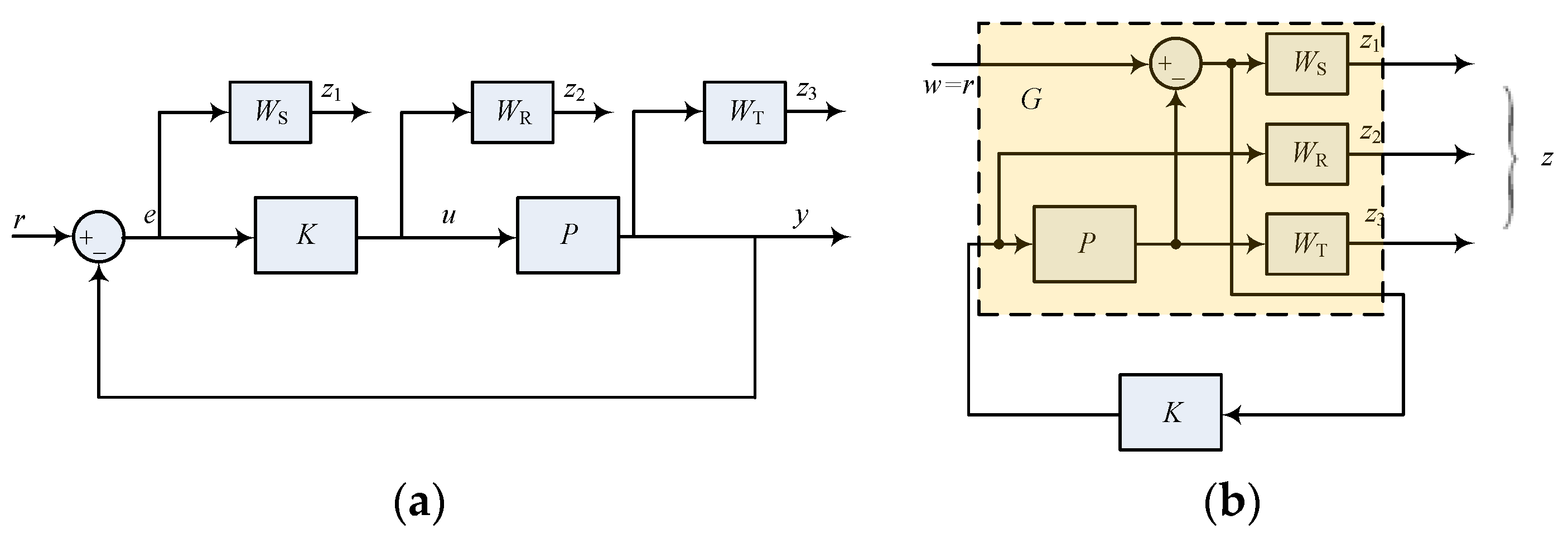
3. Weighting Function and Its Influence

Section 2 shows that the performance weighting function plays an important role in H_∞ controller design. In this section, the weighting function with adjustable parameters is proposed. Moreover, the influence of the parameters on the system dynamics is discussed.

3.1. Selection of Performance Weighting Function

3.1.1. Weighting W_S

W_S is the weighting function of the sensitivity function S. In the RTHS used for earthquake engineering, the frequency of the commanded signals and disturbances is generally very low. Hence, to track the reference signal with high accuracy and to suppress the external disturbances, the sensitivity function S should be small enough over the low-frequency range, while in the high-frequency band beyond the command signal, there are no additional restraints for the sensitivity function S. Therefore, the weighting function W_S should have a high gain over the low-frequency range. Hence, W_S can be selected as

$$W_S=\frac{as+b{\omega }_{\mathrm{d}}}{s+c}$$

(6)

where a, b, and c are adjustable parameters, and ω_d is the desired bandwidth of the system. The singular value of W_S⁻¹ is shown in Figure 3. It is seen from the figure that, if c is small enough, that the sensitivity function S will tend to zero when the frequency is not very high, which means that the controlled system can realize the command perfectly. Typically, –60 dB is small enough for the sensitivity function S when the frequency is low; hence, it is recommended that c is less than 0.01.

Figure 3. Singular value of W_S^−1.

3.1.2. Weighting W_T

W_T is the weighting function of the complementary sensitivity function T, which represents the characteristic of the multiplicative uncertainties [24]. Hence, the weighting W_T can be selected as

$$\sigma \left(\frac{G\left(j\omega \right)}{G_0\left(j\omega \right)}-1\right)<\sigma \left(W_T\left(j\omega \right)\right),\forall \omega$$

(7)

where G is the actual plant, G₀ is the nominal or analytical plant, and σ is the singular value. Once W_T is determined, it can remain unchanged, because it is related to the model of the control plant.

In RTHS, it is expected that T should be close to 1 to achieve the reference command, especially over the concerned frequency band. Afterward, T should be small enough to suppress the modeling errors over the high-frequency range, which will also diminish the effect of measurement noise. Furthermore, if the gain of W_T decreases quickly over the high-frequency range, the measurement noise will be suppressed effectively. Hence, for practical purposes, the recommended form of function W_T is given by

$$W_T=h{s}^2+ms+n$$

(8)

where h, m, and n are adjustable parameters. It should be noted that W_TP should be a rational function. If not, the form in Equation (8) should be modified. Examples can be found in the subsequent sections.

3.1.3. Weighting W_R

The weighting W_R is associated with the additive uncertainties [24]. Typically, the weighting W_R is introduced to satisfy the premises of the H_∞ control theory. While it is seen in Section 2, W_R is the weighting of the controller sensitivity R, which is related to the command sent to the servo valve in RTHS. A high controller gain will destabilize the system due to measurement noise. Hence, to suppress the maximum magnitude of the controller, the weighting W_R can be selected as a small constant. The weighting W_R can be eliminated.

3.2. Influence on the System Dynamics

In RTHS, it is expected that the servo-hydraulic actuator can realize the desired displacement command quickly and precisely. Hence, to give guidance on weighting function selection, the influence of the parameters in the weighting function on the dynamics, namely the settling time, overshoot, and steady-state error, were investigated in this subsection. The control plant, from the controller output u to measurement displacement y, was taken as

$$P=\frac{20.99}{s+1.418}.$$

(9)

By several trials, the weighting functions were selected as follows:

$$W_S=\frac{0.0475s+170.1}{s+0.001},W_T=\frac{2500(s+250\left)\right(s+14.14)}{{(s+1.571\times {10}^4)}^2},W_R=0.001.$$

(10)

It should be noted that as the control plant is a first-order transfer function, the form of the weighting function W_T is modified to guarantee that W_TP is a rational function. The step response was obtained and is shown in Figure 4. It is seen that the controlled system could respond to the reference command quickly, and there was no steady-state error, indicating a perfect tracking performance.

Figure 4. Step response of the H_∞-controlled system.

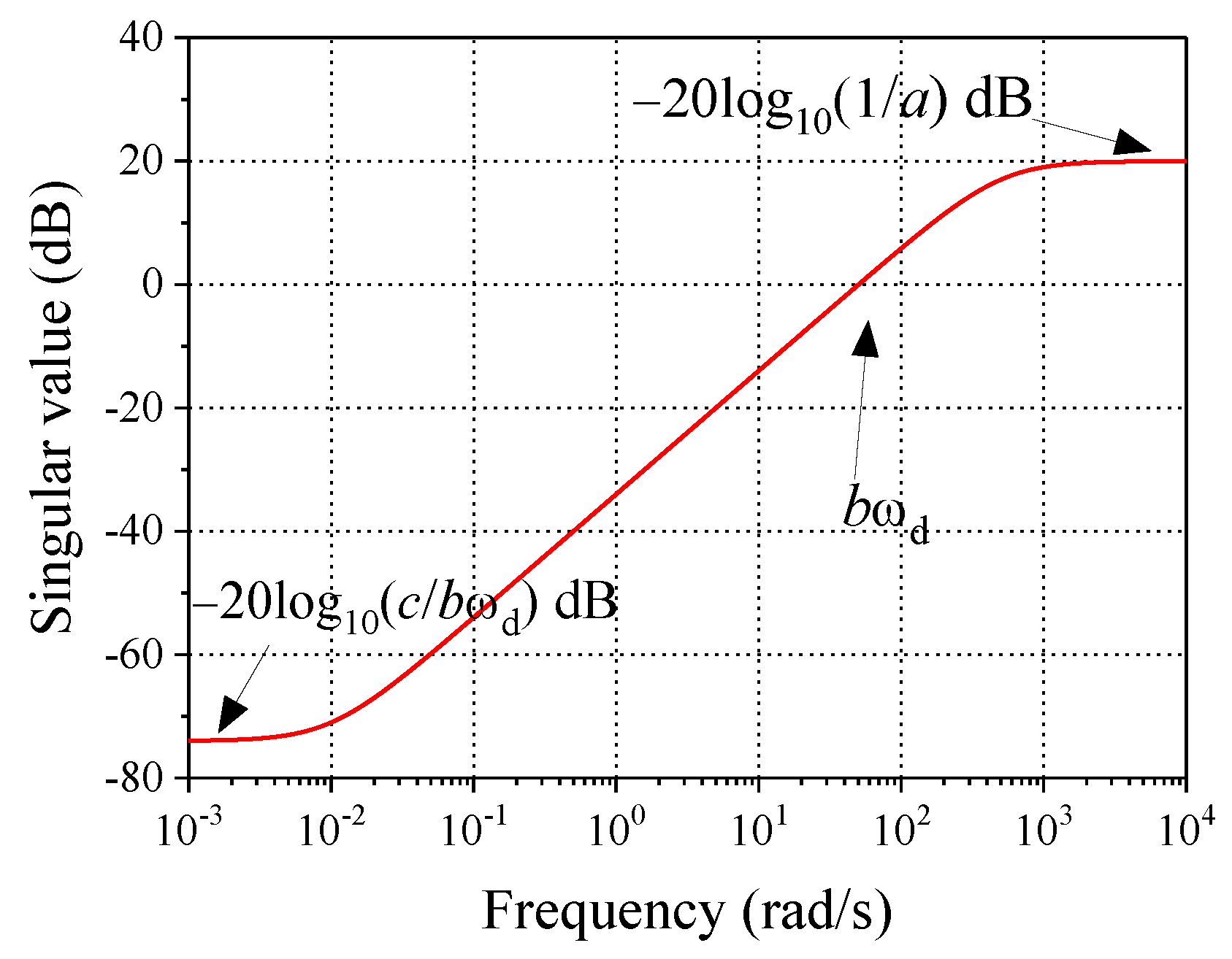
3.2.1. Influence of W_S

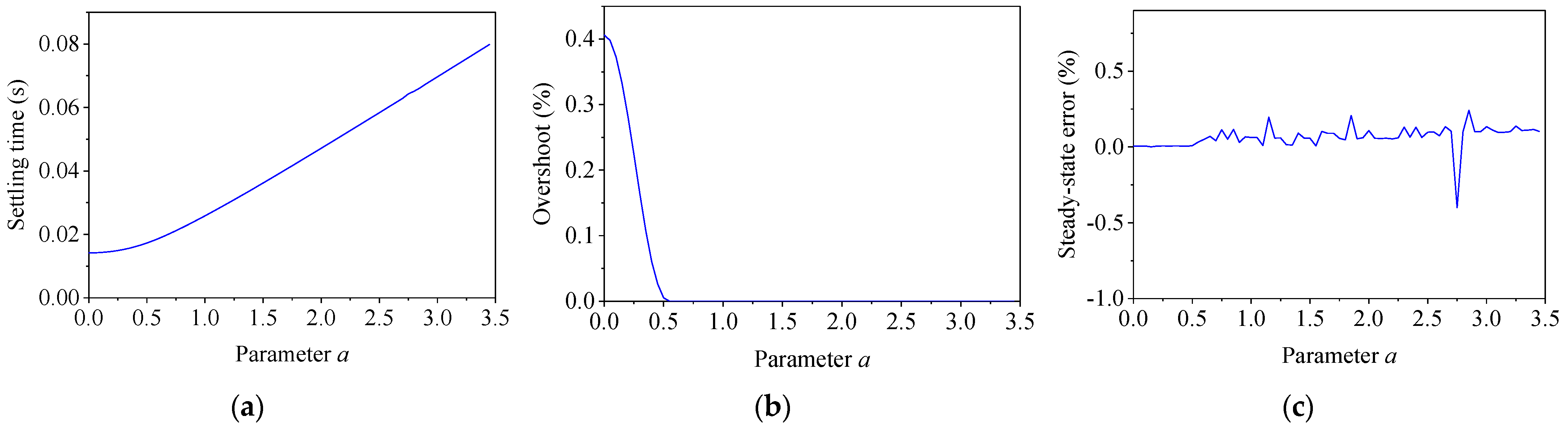
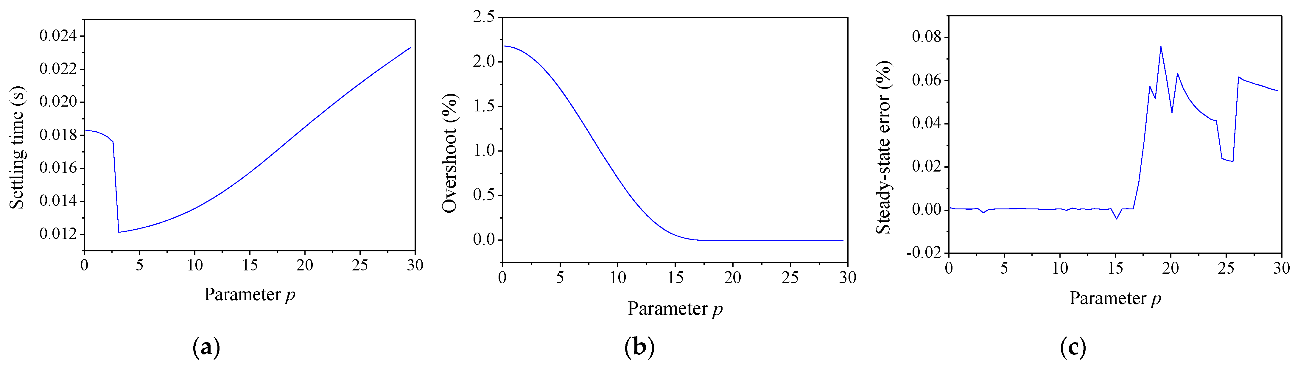
• Parameter a in W_S

To analyze the influence of the parameter a on weighting function W_S, the other parameters in the weightings were kept unchanged. By changing a from 0 to 3.5, the dynamics were calculated via the step response, which is shown in Figure 5. It is seen from the figure that with the increase in parameter a, the settling time grew rapidly, while the overshoot decreased quickly. The steady-state error almost remained the same. Hence, it is recommended that a small positive value should be used for parameter a.

Figure 5. Effect of parameter a on W_S. (a) Settling time; (b) overshoot; (c) steady-state error.

2.

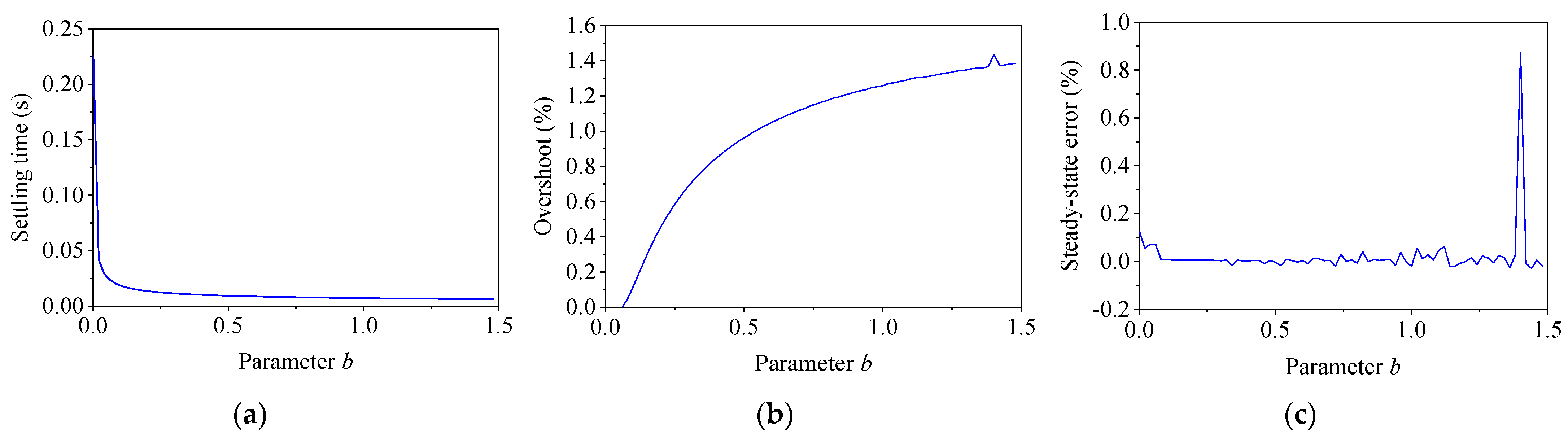
Parameter b in W_S

When designing the weightings in Equation (10), the desired system band was 20 Hz and b was 1.35. To analyze the influence of the parameter b on weighting function W_S, the other parameters in the weightings were kept unchanged. By changing b from 0 to 1.5, the dynamics were calculated by the step response, which is shown in Figure 6. It is seen in Figure 6 that when parameter b was less than 0.1, with the increase in parameter b, the settling time decreased rapidly, while the overshoot almost remained unchanged. When parameter b was larger than 0.1, with the increase in parameter b, the settling time decreased very slowly, while the overshoot increased quickly. The steady-state error almost remained unchanged. It is seen in Equation (6) and Figure 3 that with the increase in b, the system bandwidth widened, resulting in the response speed accelerating and the overshoot increasing. Hence, it is recommended that a larger b should be used if one expects a faster response speed.

Figure 6. Effect of parameter b on W_S. (a) Settling time; (b) overshoot; (c) steady-state error.

3.

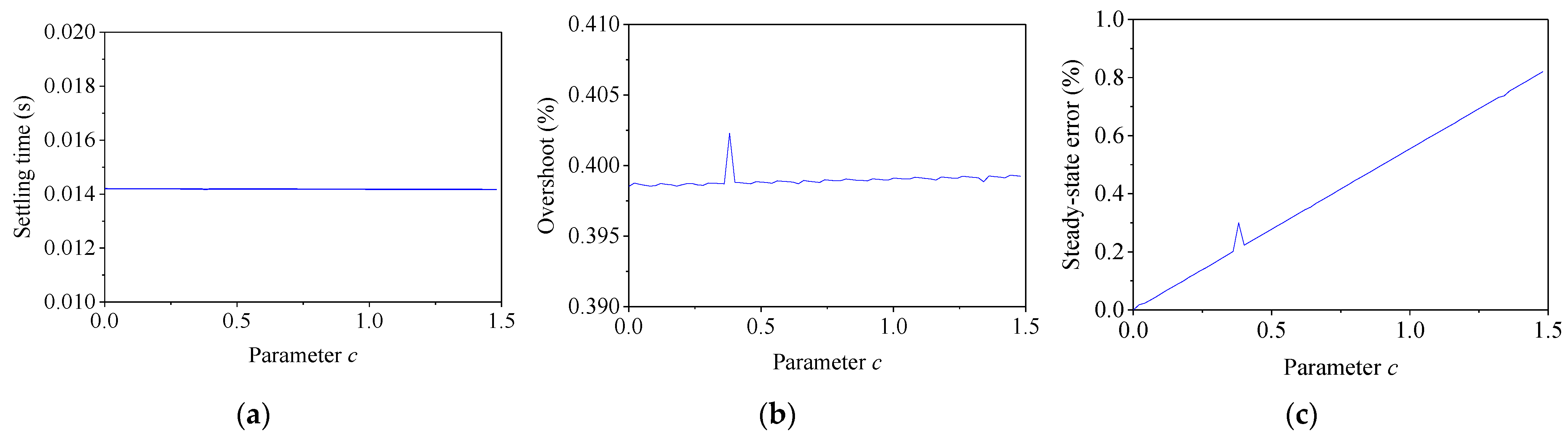
Parameter c in W_S

The parameter c was changed from 0 to 1.5 to investigate its influence, while the other parameters in the weightings were kept unchanged. The dynamics were calculated by the step response, which is shown in Figure 7. It is seen that with the increase in parameter c, the settling time and the overshoot almost remained unchanged, while the steady-state error increased. Hence, it is recommended that the parameter c should be small enough to eliminate the steady-state error, which is very important to RTHS.

Figure 7. Effect of parameter c on W_S. (a) Settling time; (b) overshoot; (c) steady-state error.

3.2.2. Influence of W_T

For convenience of analysis, the weighting function W_T in Equation (10) can be rewritten as

$$W_T=\frac{0.0225s^2+5.9431s+79.5216}{{\left(0.003s+47.1239\right)}^2}.$$

(11)

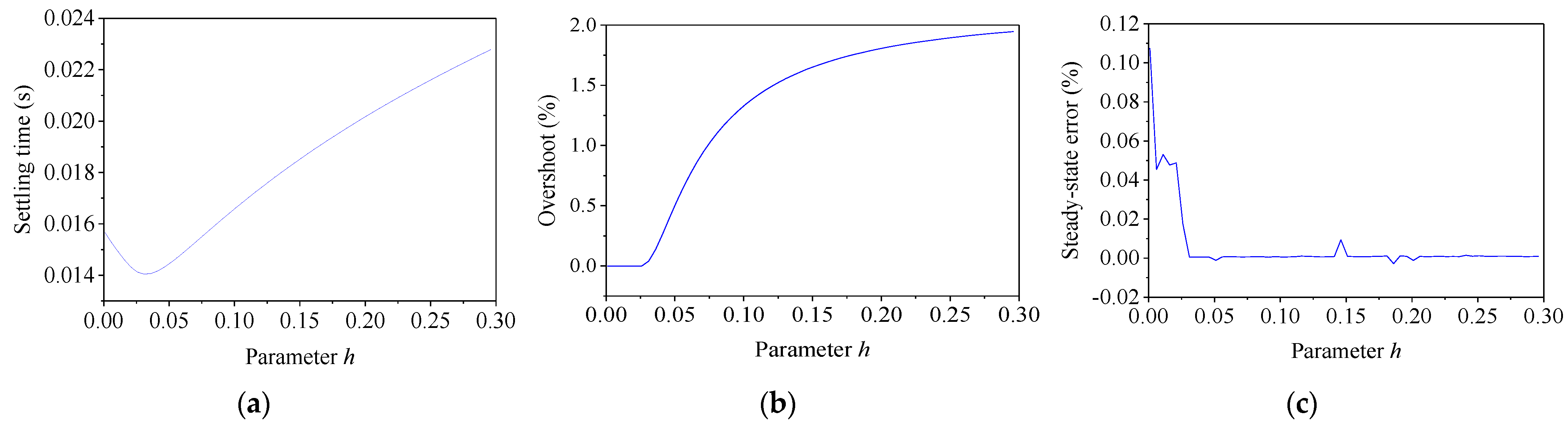
• Parameter h in W_T

Keeping the other parameters in the weightings unchanged, the parameter h was varied from 0 to 0.3 to examine its influence. The dynamics were calculated via the step response, which is shown in Figure 8. With the increase in parameter h, the settling time decreased first and then increased rapidly. The overshoot almost remained unchanged at the beginning and then increased quickly, while the steady-state error decreased quickly and then remained unchanged.

Figure 8. Effect of parameter h on W_T. (a) Settling time; (b) overshoot; (c) steady-state error.

2.

Parameter m in W_T

To analyze the influence of the parameter m on weighting function W_T, the other parameters in the weightings were kept unchanged. By changing m from 0 to 30, the dynamics were calculated by the step response, which is shown in Figure 9. With the increase in parameter m, the settling time almost remained unchanged first and then decreased quickly. Then, the settling time increased with the increase in parameter m. The overshoot decreased with the increase in parameter m, and then almost remained unchanged regardless of how the parameter m increased. Meanwhile, the steady-state error remained unchanged first and then fluctuated at a relatively high value.

Figure 9. Effect of parameter m on W_T. (a) Settling time; (b) overshoot; (c) steady-state error.

3.

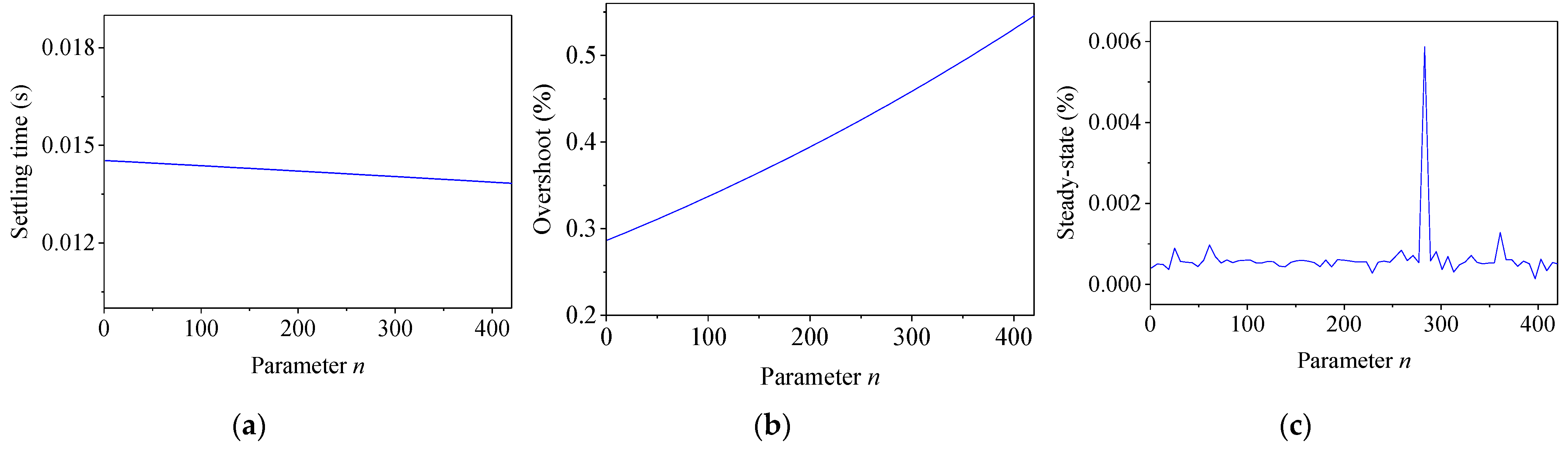
Parameter n in W_T

By varying the parameter n from 0 to 450, the dynamics were calculated via the step response correspondingly, which are shown in Figure 10. It is seen that with the increase in parameter n, the settling time and steady-state error varied in a very small range, which could be viewed as unchanged. Meanwhile, the overshoot increased with the parameter n.

Figure 10. Effect of parameter n on WT. (a) Settling time; (b) overshoot; (c) steady-state error.

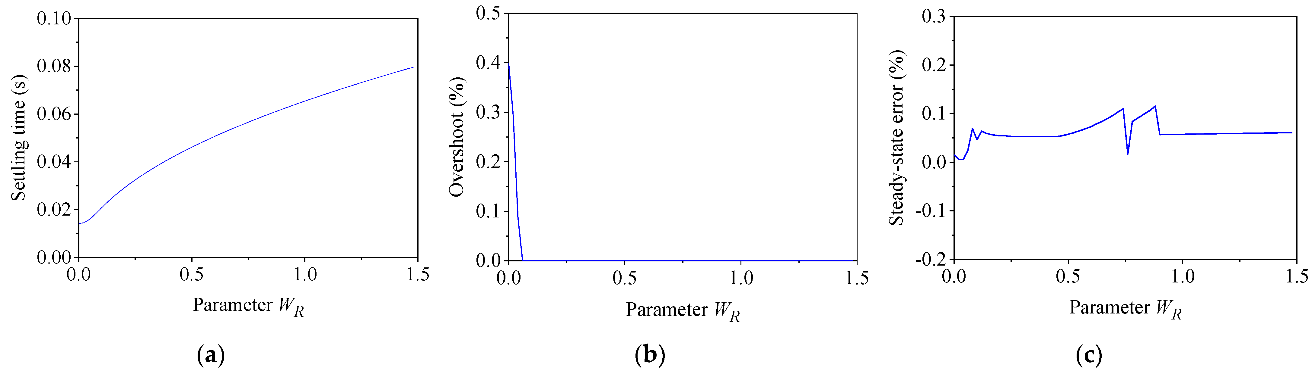
3.2.3. Influence of W_R

The weightings W_S and W_T were kept unchanged, and the weighting W_R was varied from 0 to 1.5. The dynamics were calculated via the step response, which is shown in Figure 11. With the increase in weighting W_R, the settling time increased. When the weighting W_R increased in a very small range near zero, the overshoot decreased quickly. Then, the overshoot almost remained at zero with the increase in W_R. The steady-state error fluctuated at a relatively small value. Hence, it is recommended that a small positive number is used for weighting W_R.

Figure 11. Effect of W_R. (a) Settling time; (b) overshoot; (c) steady-state error.

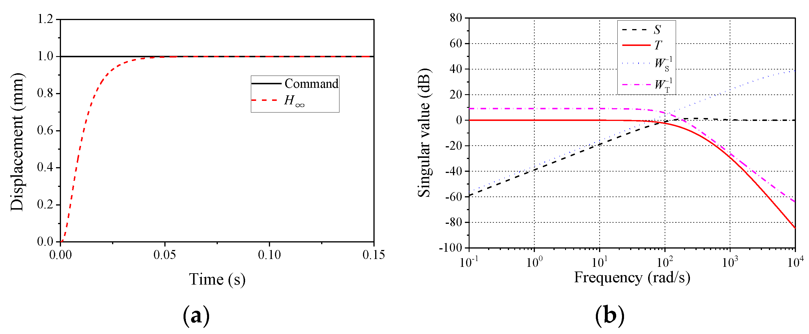
4. Numerical Validation

In this section, a nonlinear model of the servo-hydraulic actuator [25] was employed to validate the effectiveness of the proposed H_∞ control method used for RTHS.

Typically, the H_∞ controller is designed by employing a nominal analytical model of the physical testing system, in which the PS is included. Hence, a linear model of the servo-hydraulic actuator, or nominal plant, is obtained from the nonlinear model for design convenience, which is given by

$$P(s)=\frac{2\beta A_p{k}_0}{M_{E}V{s}^3+(C_{E}V+2\beta k{M}_E{k}_0)s^2+(K_{E}V+4\beta A_p^2+2p{A}_p^2+2k\beta C_E{k}_0)s+2k\beta K_E{k}_0}.$$

(12)

where the symbols and their values are listed in Table 1. The damping coefficient C_E is calculated by the damping ratio and natural frequency of the specimen. Then, the transfer function of the nominal model is

$$P\left(s\right)=\frac{7.748\times {10}^6}{s^3+165.7s^2+3.706\times {10}^{5}s+5.235\times {10}^5}.$$

(13)

Table 1. Values of system parameters for simulation [25].

Item	Parameter	Value	Parameter	Value
Servovalve	Natural frequency	816.81 rad/s	Damping ratio	0.7
	Servo-valve gain k0	1.0674 m2/s	Supply pressure p	19.995
Actuator	Piston area Ap	0.0248 m2	Volume V	0.0069 m3
	Effective bulk modulus of oil β	677.8 MPa	Pressure difference feedback gain k	0.0002
Specimen	Mass ME	56.289 kg	Damping ratio	0.05
	Stiffness KE	2276.3 kN/m

It should be noted that the units have been transformed into the international system of units.

4.1. Robustness Investigation

In a real application, there are differences between the nominal model and the physical testing system, and the characteristics of the PS will vary during RTHS. Hence, the robustness of the H_∞ controller was investigated numerically in this section.

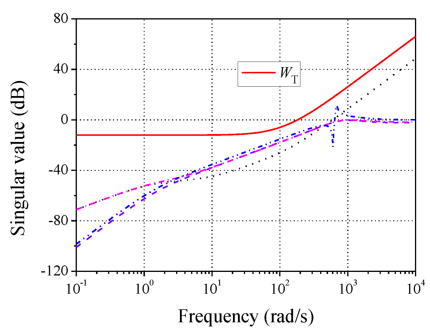
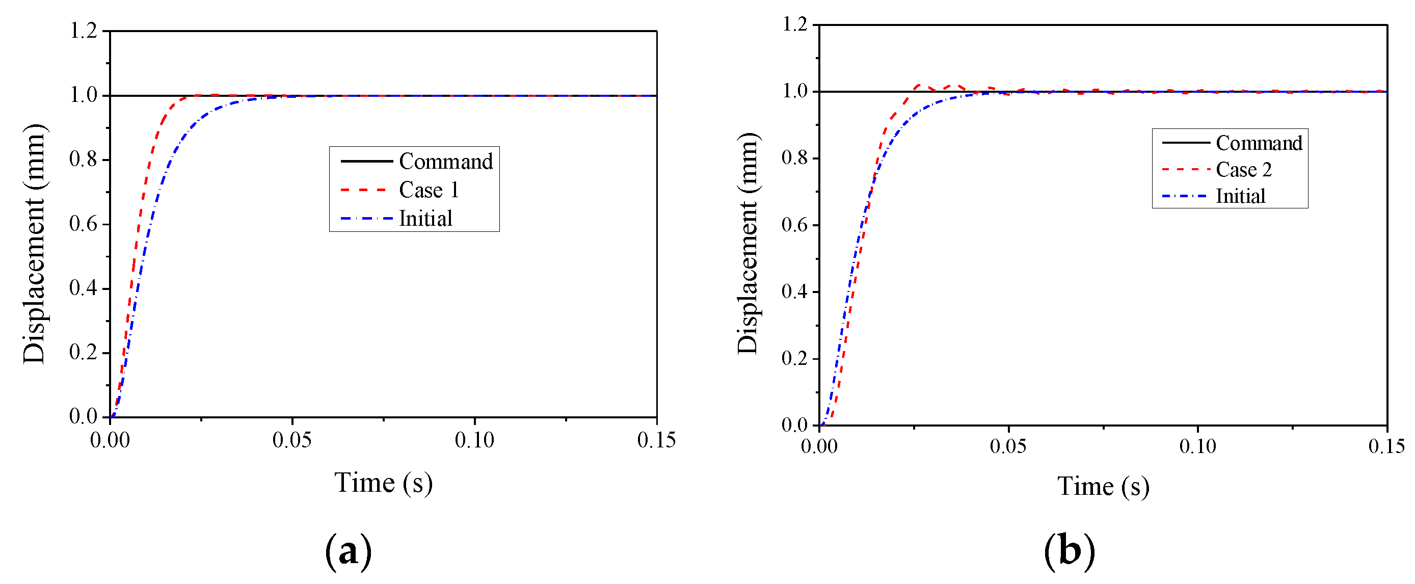
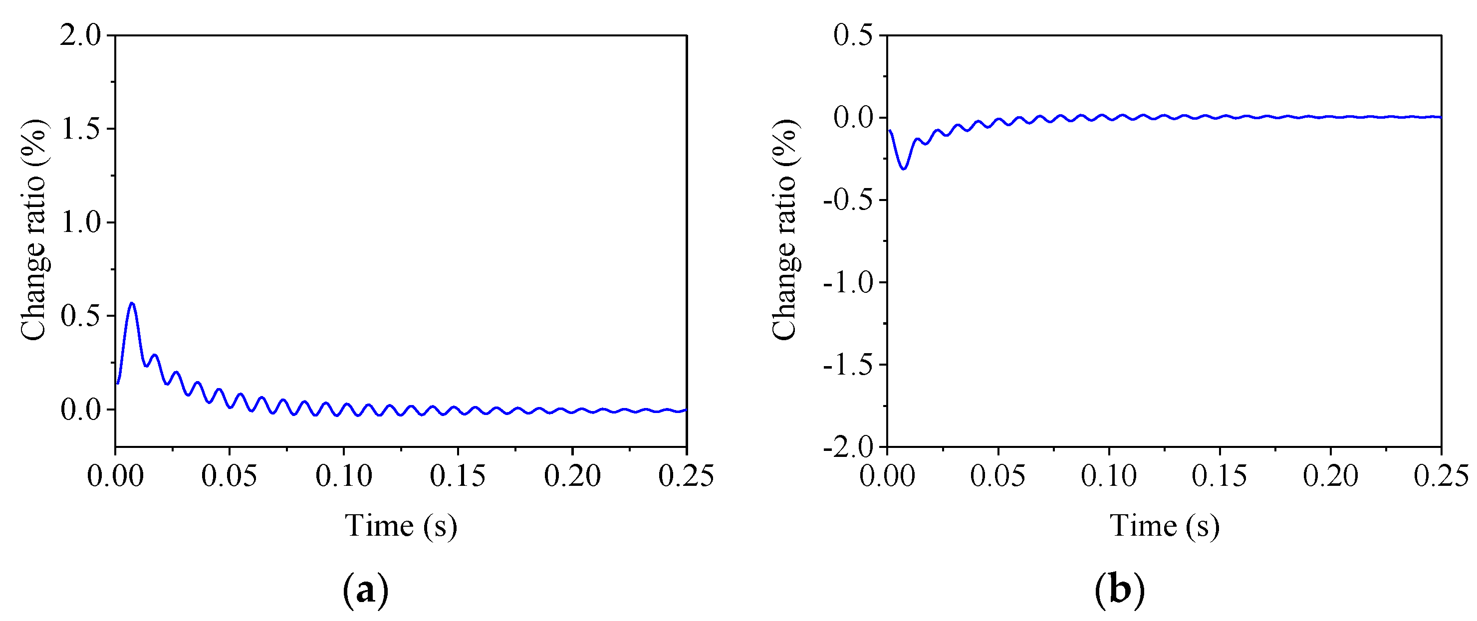
4.1.1. Modeling Uncertainties

• Controller design

When designing the H_∞ controller, the modeling uncertainties and measurement noise should be considered first, followed by the dynamics of the controlled system. Hence, it is recommended that the designed order of the weighting function is W_T, W_S, and W_R.

To determine the modeling uncertainties, a series of linear numerical models of the nonlinear model were calculated. Then, the uncertainties were obtained, whose singular values are shown in Figure 12. Later, the weighting W_T can be designed. It is seen in the figure that the modeling error was very small when the frequency was not very high; then, the modeling uncertainties increased with the frequency. Hence, the weighting W_T should cover the uncertainties over all the frequency ranges. Through several trials, the expression for W_T was given by

$$W_T\left(s\right)=2\times {10}^{-5}{s}^2+0.005s+0.25$$

(14)

Figure 12. Modeling uncertainties and weighting function W_T.

Subsequently, the dynamics of the controlled system were considered. It is expected that the controlled system should respond to the command quickly and without a steady-state error. Hence, the other two weightings were determined after several trials, which were

$$W_S\left(s\right)=\frac{0.01s+63}{s+0.001},W_R=0.1$$

(15)

Eventually, a feasible solution was reached, and the H_∞ central controller was

$$K\left(s\right)=\frac{\mathrm{7,731,236.8628}(s+1.413)(s^2+164.3s+3.704\times {10}^5)}{(s+1.021\times {10}^6\left)\right(s+1171\left)\right(s+568.5\left)\right(s+0.001)}$$

(16)

Afterward, the performance of the controlled system was examined through performance curves and the step response, which are given in Figure 13. A fast response speed is observed in Figure 13a, and there is no steady-state error. It can also be seen from Figure 13b that the complementary sensitivity function T was almost identical to 1 when the frequency was less than 10 Hz, indicating that the controlled system could track the command very well. It is seen in the figure that the curves of the sensitivity function S and complementary sensitivity function T were below the weighting functions W_S⁻¹ and W_T⁻¹, respectively, indicating that the selected weighting function could meet the robust performance [24]. Moreover, over the concerned frequency, the sensitivity function S was far less than 1, indicating that the controlled system exhibited a strong robustness considering the disturbance.

Figure 13. Performance of the controlled system. (a) Step response; (b) performance curve.

• Modeling errors

To investigate the robustness of the H_∞ controller to modeling uncertainties, two cases were considered here. For the first case, the multiplicative uncertainties of 50% were considered, while for the second case, the controller designed employing a linear model was used for the nonlinear model. Step responses for the two cases are shown in Figure 14, and the response without any uncertainties is also given in the figure for convenience of comparison.

Figure 14. Step responses. (a) Case 1: multiplicative uncertainties; (b) case 2: nonlinear model.

It is seen in the figure that when the multiplicative uncertainties were considered, steady-state errors and overshoots were still not observed, while the settling time was less than the initial state. When the H_∞ controller was used for the nonlinear model, it was found that there were obvious fluctuations, and overshoot and steady-state errors occurred. However, the overshoot was very small (less than 0.5%), and the steady-state error tended to zero. Hence, the H_∞ controller exhibited strong robustness to modeling uncertainties.

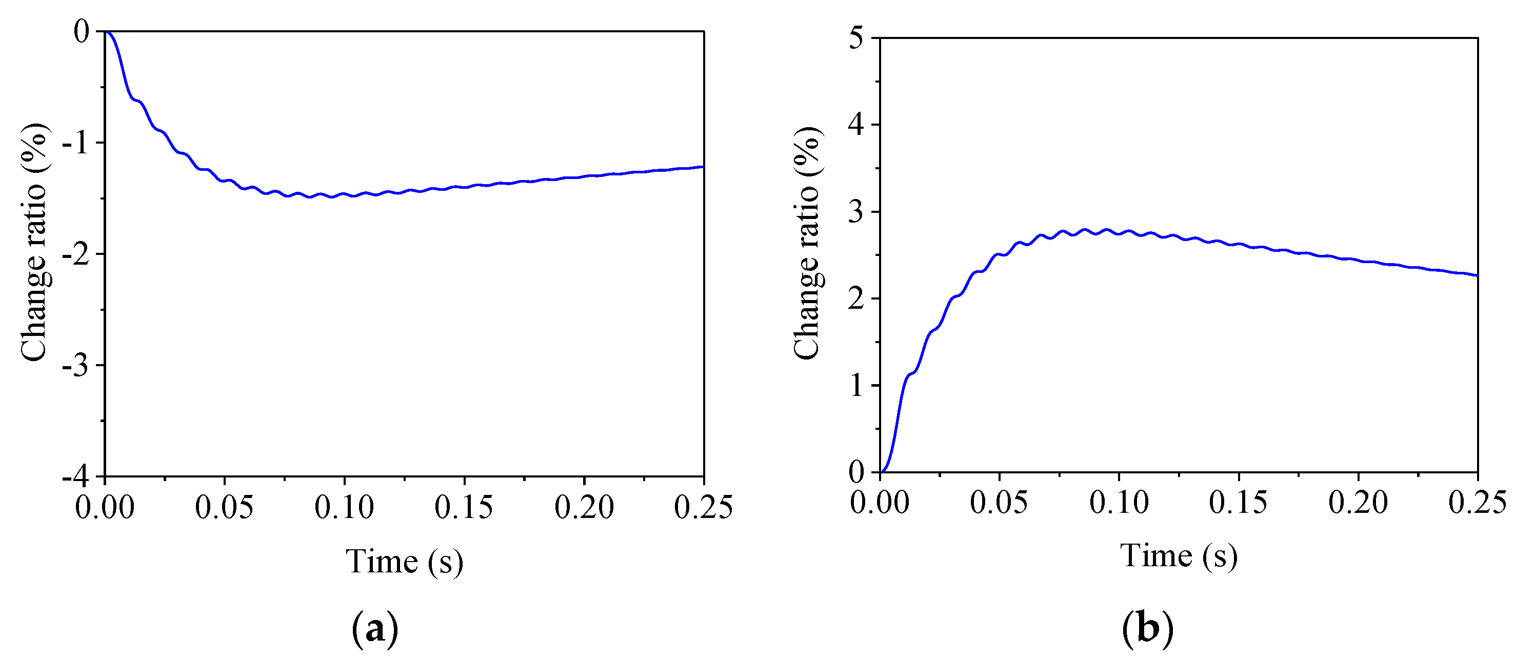
4.1.2. Variation of the Specimen

• Stiffness

Two different stiffness coefficients were considered for the PS, 1.5 and 0.1 times the initial one, respectively. The time histories of the change ratio under the step response are given in Figure 15. It is seen from the figure when the stiffness coefficient varied, the steady-state error occurred. The change ratio for the stiffness decrease was smaller than that for the stiffness increase, and they were within the acceptable range. Hence, the H_∞ controller was robust to the variation in stiffness.

Figure 15. Change ratio of step response for different stiffnesses. (a) K_E = 0.1K_E0; (b) k_E = 1.5K_E0.

• Damping

To assess the robustness of the H_∞ controller, two different damping ratios, 0.1 and 1.5 times the initial one, respectively, were considered for the PS. The time histories of the change ratio under the step response are given in Figure 16. It is found that the change ratios were negligible compared to those in Figure 15. With time, the change ratio tended to zero, which means that the steady-state error was zero. This indicates that the damping characteristics had limited influences on the step responses, and the H_∞ controller exhibited a strong robustness.

Figure 16. Change ratio of step response for different stiffnesses. (a) C_E = 0.1C_E0; (b) C_E = 1.5C_E0.

4.2. Virtual RTHS

In this section, virtual RTHSs were conducted on a single-degree-of-freedom (SDOF) structure. The mass was 1200.8 kg, the structural stiffness was 2276.3 kN/m, and the damping ratio was 5%. A nonlinear PS was employed, of which the mass and stiffness of the PS were 56.6384 kg and 2276.3 kN/m, respectively, the yield displacement was 7.6 mm, and the stiffness coefficient after yield was 0.12. The earthquake excitation was El Centro (NS, 1940), whose peak ground acceleration (PGA) was scaled to 0.16g. In the virtual hybrid simulation, the α method [26] was adopted to solve the equation of motion, and the time integral was 0.01 s. A pure dynamic analysis of the whole structure was performed to serve as an exact reference solution, where the stepwise integral method was CDM-RST [25], and the time step was 0.01 s. Due to the PS being changed, the controller was re-designed, and the controller was:

$$K=\frac{\mathrm{14,893,750.8909}(s+2.094\times {10}^4)(s+1.047\times {10}^4)(s+1.413)(s^2+164.3s+3.704\times {10}^5)}{(s+1.305\times {10}^6\left)\right(s+2.096\times {10}^4\left)\right(s+1.031\times {10}^4\left)\right(s+1196\left)\right(s+669.9\left)\right(s+0.001004)}$$

(17)

The time histories of displacement obtained by virtual RTHS were compared with those of the reference solution, which is shown in Figure 17. It is seen in the figure that a shifting was observed for the displacement due to the yielding of the structure. However, the responses were in good agreement with those of the reference solution under the earthquake excitation.

Figure 17. Displacement time histories for virtual RTHS.

5. Experimental Validation

5.1. Overview of the Test

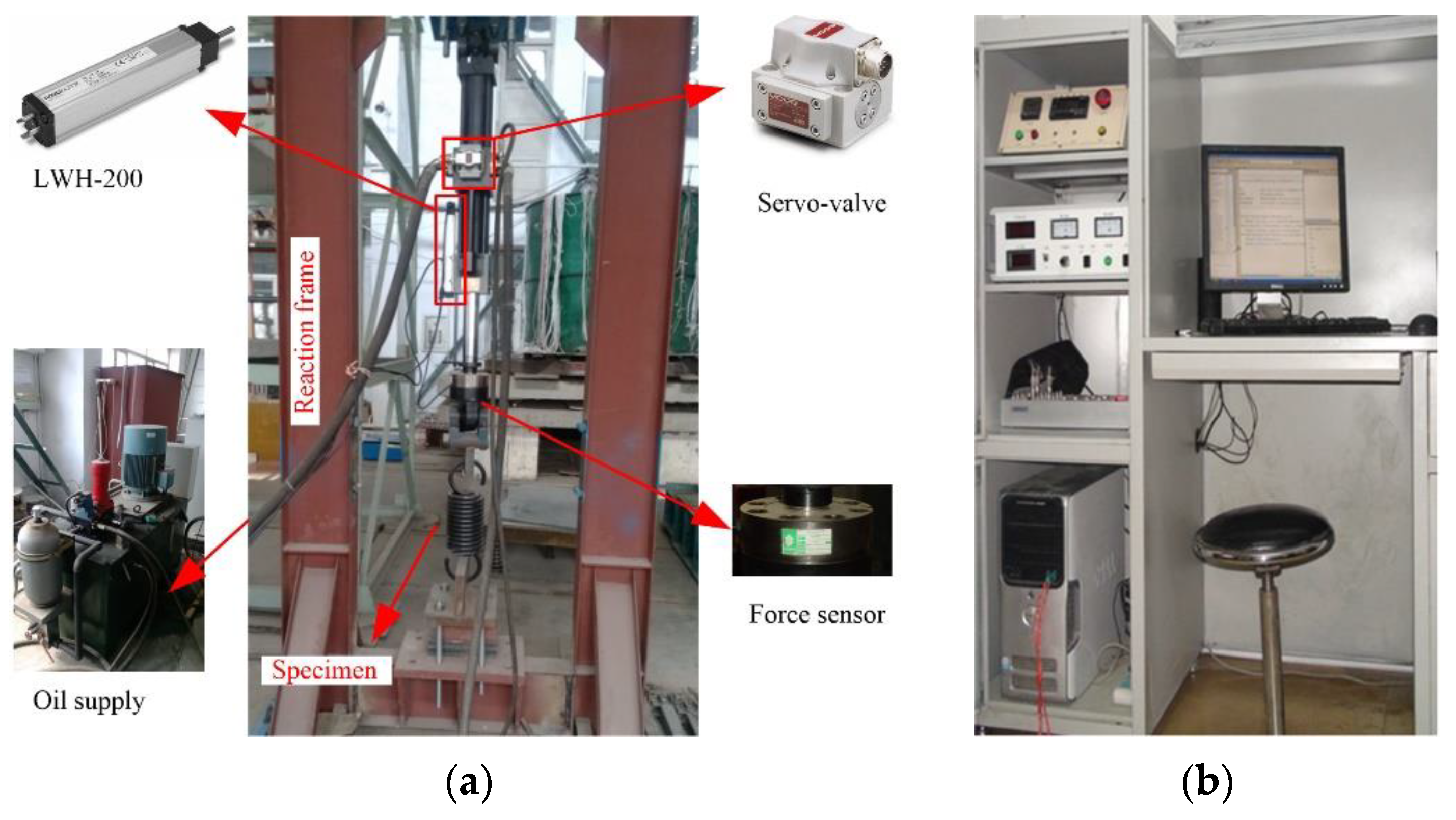
5.1.1. Experimental Setup

To validate the effectiveness of the proposed H_∞ control method, actual real-time hybrid simulations were conducted on an SDOF structure. The loading system at the Structural and Seismic Testing Center of Harbin Institute of Technology was employed, which consists of an FTS system and a dSPACE 1104 board. The FTS system comprises a servo-hydraulic actuator, displacement sensor, force sensor, and servovalve. The displacement sensor is an LWH-200 with a maximum stroke of 200 mm, which is produced by Novotechnik. The force sensor is PSD-5tSJTT with a capacity of 5 T, which is produced by Vishay. The servovalve is MOOG-761-3005, produced by Moog. The experimental setup is shown in Figure 18.

Figure 18. Loading system setup. (a) FTS system; (b) control hardware and system.

Considering the restraints of the loading system, a spring was taken as the specimen and was loaded in the axial direction. In RTHS, the central difference method was adopted to solve the equation of motion, and the time integral was 0.02 s. The equation of motion solved by the LSIM command in MATLAB served as the exact reference solution, where the time step was 0.02 s.

To diminish the effect of measurement noise, an elliptic filter was designed by the digital filter design module, with stop frequencies of 100 and 30 Hz for displacement and force, respectively. The sampling time for the filter was 1000 Hz.

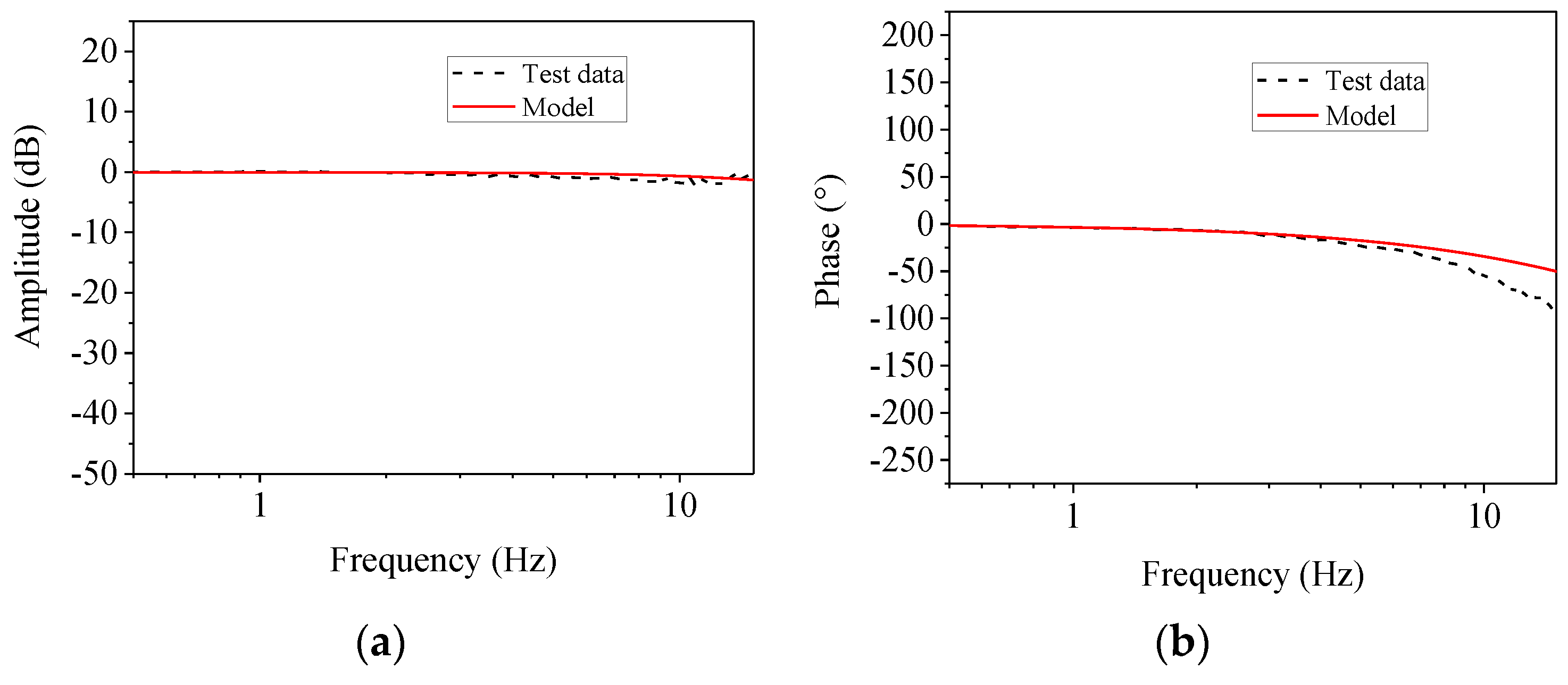
5.1.2. Controller Design

Similar to that used in Section 4, the analytical model was established theoretically using the technical index of the servo-hydraulic actuator, which is provided by the manufacturer. The transfer function from u to y is

$$P=\frac{4\beta k_0{A}_p}{\left(4\beta A_p^2+4p{A}_p^2+V{K}_e\right)s+4\beta k{k}_0{K}_E}$$

(18)

where the parameters are listed in Table 2. Hence, the numerical model is given by

$$P\left(s\right)=\frac{33.74}{s+0.5739}$$

(19)

Table 2. Values of system parameters.

Parameter	Value	Parameter	Value
Servo-valve gain k0	0.0512 m2/s	Supply pressure p	19.995
Piston area Ap	0.0015 m2	Volume V	0.0043 m3
Effective bulk modulus of oil β	677.8 MPa	Pressure difference feedback gain k	0.0002

The mathematical model in between the input and output in the frequency domain is shown in Figure 19. It is seen in Figure 19a that within the frequency range of interest, the model was in good agreement with the test data, while for the phase, differences were observed when the frequency became large. However, the analytical model can reflect the major dynamics of the actual testing system.

Figure 19. Model validation. (a) Magnitude; (b) phase.

The weighting functions were determined using the recommended method given in Section 3. After several trials, they were selected as

$$W_S=\frac{0.05s+62.83}{s+0.01},W_T=\frac{833.3333(s+805\left)\right(s+19.51)}{(s+2.09\times {10}^4\left)\right(s+1.05\times {10}^4)},W_R=1\times {10}^{-6}$$

(20)

Eventually, a feasible solution was achieved and the controller was

$$K\left(s\right)=\frac{7.6251\times {10}^8(s+2.094\times {10}^4\left)\right(s+1.047\times {10}^4\left)\right(s+0.5739)}{(s+2.812\times {10}^{10})(s+0.01048)(s^2+1892s+1.086\times {10}^2)}$$

(21)

It should be noted that the H_∞ controller was designed in the continuous-time domain, while the dSPACE is a digital sampling system. Hence, the H_∞ controller was converted to discrete form by the c2d command in MATLAB. The discrete method was Tustin, and the sampling time was identical to that in dSPACE, namely 1000 Hz.

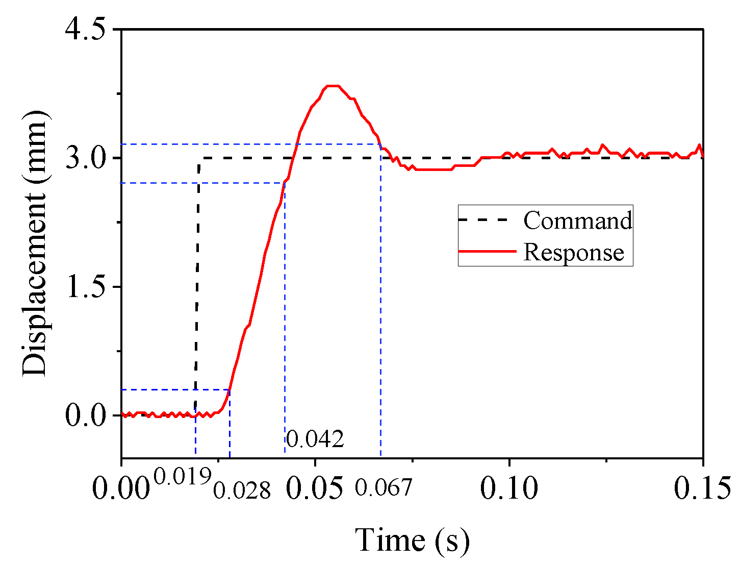
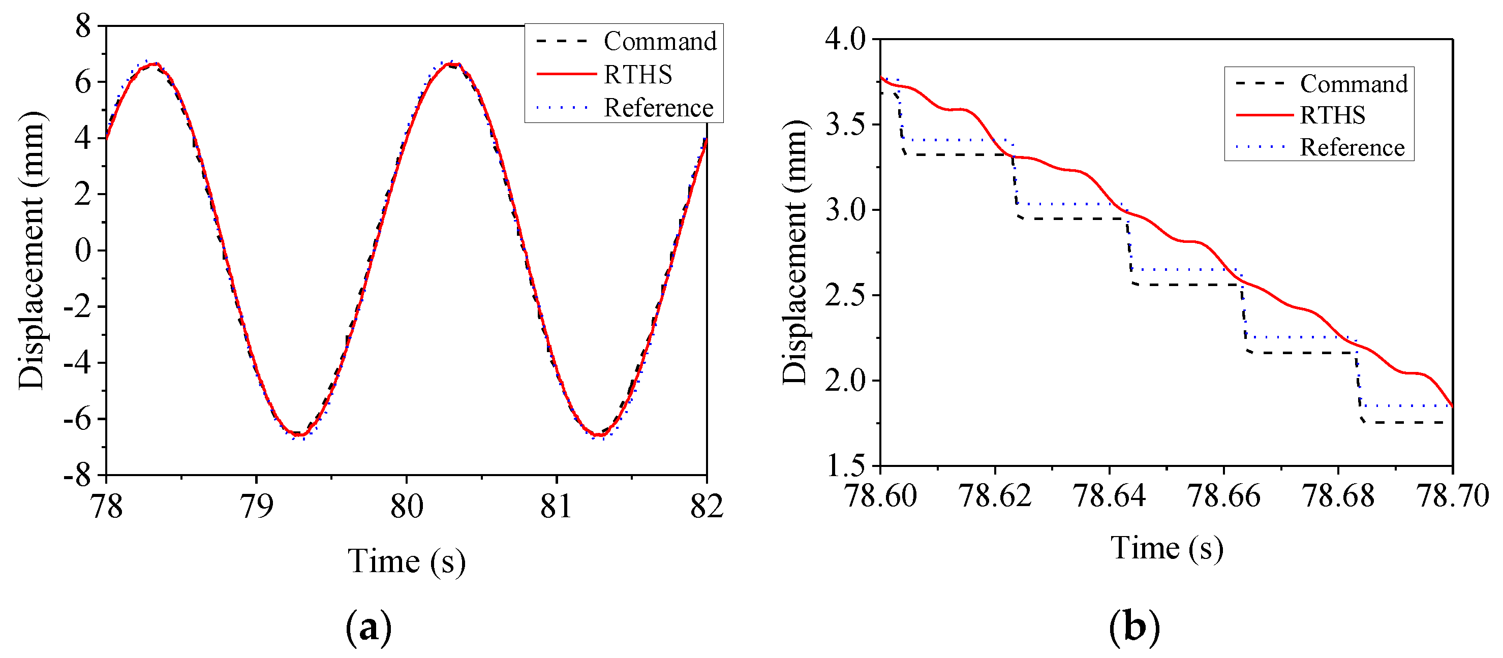
5.2. Loading System Verification

The feasibility of the designed H_∞ controller was verified first. The step response is given in Figure 20. It is seen in the figure that there was a pure delay in the system and no steady-state error. The rise and settling times were 0.018 and 0.048 s, respectively. The time of first achieving the command was 0.025 s. It seems that the H_∞ controller could not complete the RTHS. However, the step response is very rigorous, so the additional test was carried out to further verify the dynamic performance.

Figure 20. Step response with H_∞ controller.

A sinusoidal signal was discretized with a sampling time of 0.02 s, which was used as the command signal. The response is shown in Figure 21. It is seen in the figure that at the end of each step, the measurement displacements were in good agreement with the command, indicating that the H_∞ controller was suitable for RTHS.

Figure 21. Tracking performance under sinusoidal signal.

5.3. RTHS

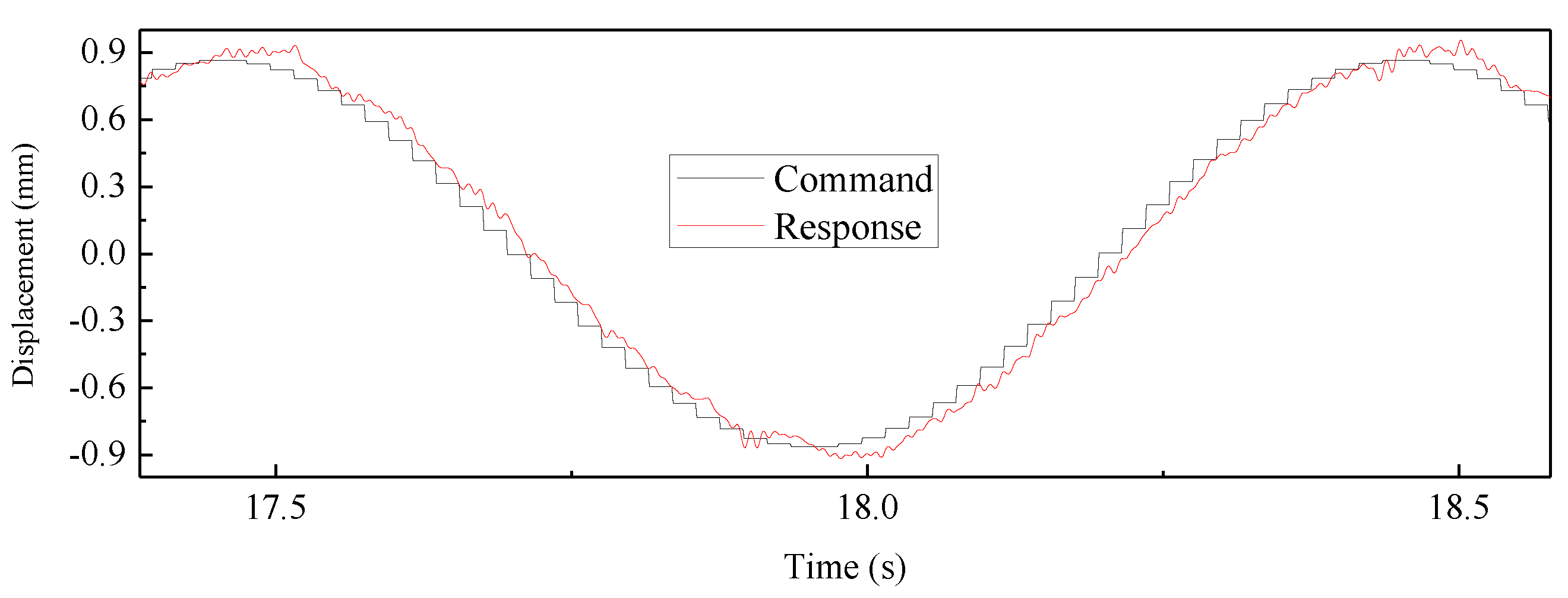
5.3.1. Sinusoidal Excitation

RTHS under sinusoidal excitation was first carried out by employing the H_∞ controller. The frequency of the excitation was 2 Hz, and the amplitude was increased slowly from 0 to 344.492 N. The period and damping ratios of the simulated structure were 1 s and 0.02, respectively. The stiffness of the NS was the same as that of the PS, which was 34 kN/m. The tracking performance of the actuator with the H_∞ controller was examined first, and the commanded and measured displacements are shown in Figure 22. It is seen in the figure that at the end of each time integration step, the displacement measurement was almost identical to that of the command. Moreover, the reference solution is also given in Figure 22. It is seen that the measured displacements were in good agreement with the reference ones.

Figure 22. Steady-state response under sinusoidal excitation. (a) Overall view; (b) enlarged view.

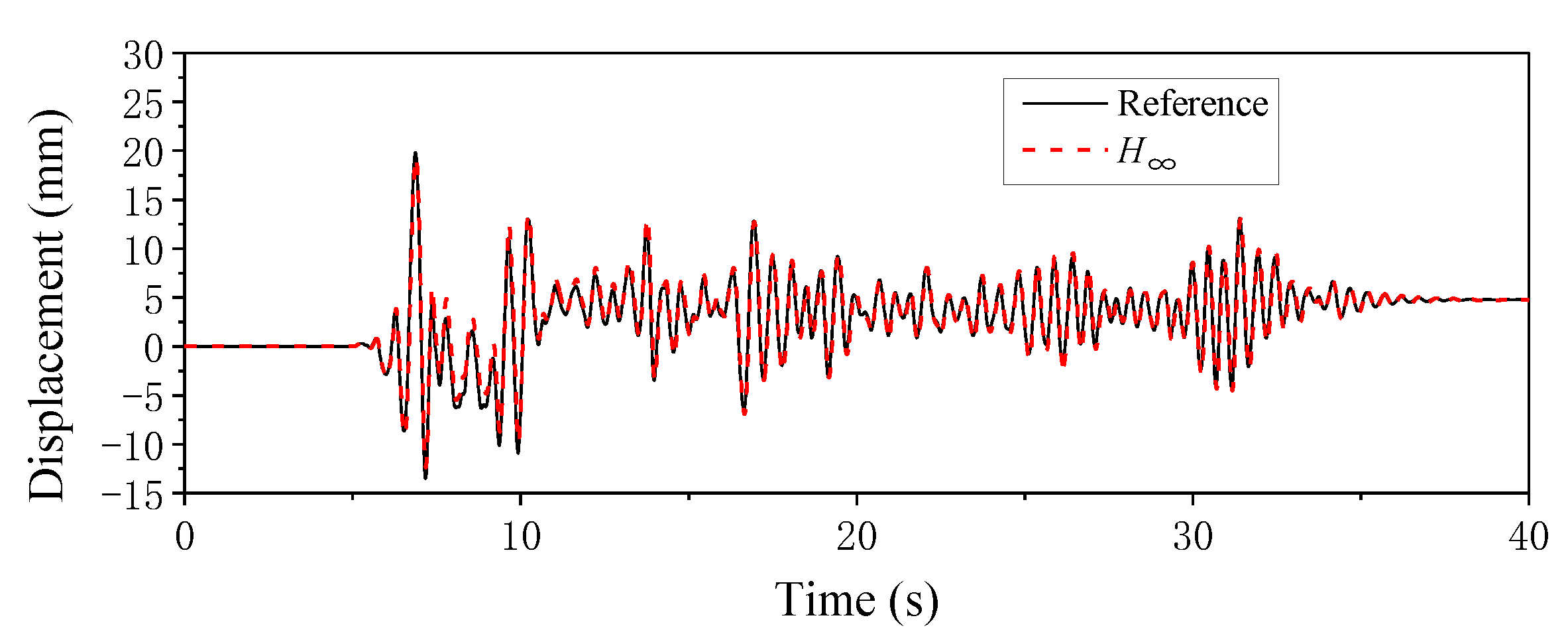
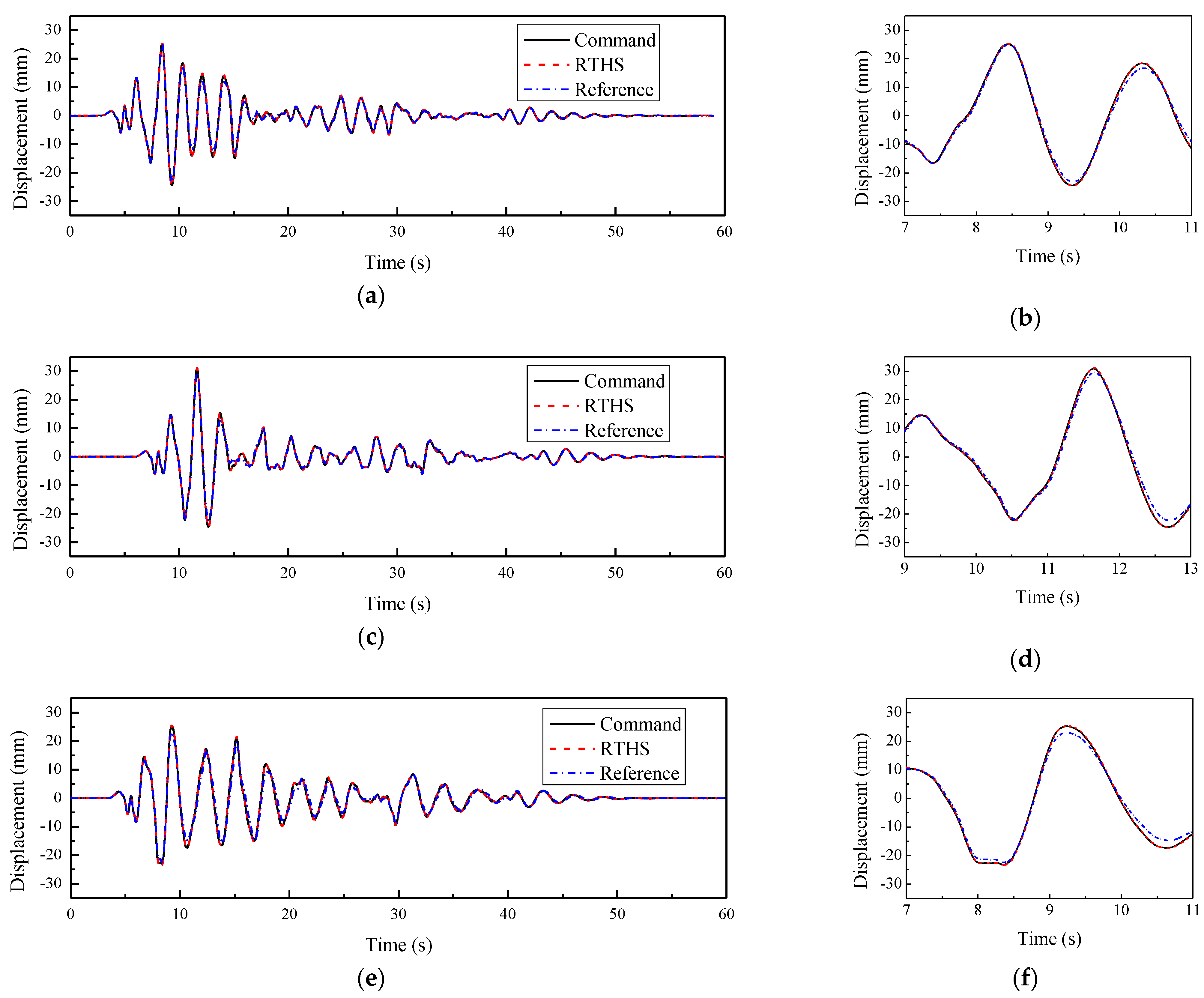
5.3.2. Earthquake

A series of RTHSs were conducted on a spring specimen with a stiffness of 35 kN/m. Three different numerical substructures, whose stiffnesses were 35, 17.5, and 0 kN/m, were considered. The damping ratio was 0.1. For the NS with a stiffness of 35 kN/m, the period was 2 s. The earthquake excitation was El Centro (NS, 1940), and the peak ground acceleration (PGA) was scaled to 50 gal. The displacement time histories, overall and enlarged view, are shown in Figure 23, together with the reference solution.

Figure 23. Displacement time histories under earthquake excitation. (a) Overall view for Case 1; (b) enlarged view for Case 1; (c) overall view for Case 2; (d) enlarged view for Case 2; (e) overall view for Case 3; (f) enlarged view for Case 3.

It is seen in the figure that the measured displacements were almost identical to the command for the three cases, indicating a perfect tracking performance of the H_∞-controlled system. They were further verified by the RMSE collected in Table 3.

Table 3. Stiffness of NS and RMS error of hybrid simulation.

Case	Stiffness of NS	RMSE (%)
		Tracking	RTHS
1	35 kN/m	2.77	12.47
2	17.5 kN/m	3.04	13.07
3	0 kN/m	2.31	17.96

If focusing on the displacement response and reference solution, one will find that the displacements of RTHS matched the reference well before the first displacement peak. Subsequently, differences emerged, especially at each positive or negative peak.

It is seen in the figure that the tracking performance was perfect, but the simulation results were barely satisfactory. The reason is that the measured force was not synchronized with the desired displacement. There were two different filters, which may introduce additional time delays differently.

6. Conclusions

Real-time hybrid simulation is a powerful technique to evaluate the structural performance under dynamic loads, especially for structures with velocity- or acceleration-dependent components. Due to the inherent nonlinearities of the servo-hydraulic actuator and the uncertainties in the systems, the boundary conditions between the two substructures could be realized completely. Hence, a mixed sensitivity-based H_∞ control method was proposed for RTHS. The main conclusions that could be reached are as follows.

• The principle of the H_∞ control theory was presented briefly. Theoretically, the H_∞ control strategy is an optimization problem. By introducing the performance weighting function to the feedback control system, the standard H_∞ control problem can be formulated.
• The weighting function selection method was proposed, and the influences of the weighting function on the system dynamics were discussed. Typically, W_S should be close to an integrator to eliminate the steady-state error, and a large numerator will generate a fast response speed. W_T should be determined by evaluating the model uncertainties in advance, and it should have a slope of approximately 40 dB/dec over the high-frequency range to suppress the unmodeled dynamics and measurement noise. A small positive constant value is usually used for W_R.
• The robustness of the H_∞ controller was investigated numerically. When considering the model uncertainties and characteristic variation in the specimen, the overshoot and steady-state error varied in an acceptable range, indicating the strong robustness of the H_∞ controller.
• The effectiveness and feasibility of the proposed method were validated via numerical simulations and actual RTSHs. When considering the nonlinear characteristics of the specimen, the actual modeling uncertainties, or the measurement noise, the H_∞-controlled system showed an excellent tracking performance, indicating that it is suitable to use the H_∞ controller for RTHS.

However, it should be noted that the proposed method was only validated via a linear elastic specimen, and a nonlinear physical substructure should be used to further validate the feasibility. Furthermore, as the H_∞ controller is still a feedback controller in essence, the time delay cannot be eliminated. Hence, it is necessary to combine the H_∞ controller with other strategies.

References

- Nakashima, M.; Kato, H.; Takaoka, E. Development of real-time pseudo dynamic testing. Earthq. Eng. Struct. Dyn. 1992, 21, 79–92. [Google Scholar] [CrossRef]
- Hakuno, M.; Shidawara, M.; Hara, T. Dynamic destructive test of a cantilever beam, controlled by an analog-computer. Pro. Jpn. Soc. Civ. Eng. 1969, 171, 1–9. [Google Scholar] [CrossRef]
- Nakashima, M.; Takai, H. Computer-actuator online testing using substructure and mixed integration techniques. In Proceedings of the 7th Symposium on the Use of Computers in Building Structures, Architectural Institute of Japan, Tokyo, Japan, 10–11 December 1985; pp. 205–210. [Google Scholar]
- Dermitzakis, S.N.; Mahin, S.A. Development of Substructuring Techniques for on-Line Computer Controlled Seismic Performance Testing; University of California: Berkeley, CA, USA, 1985. [Google Scholar]
- Wu, B.; Bao, H.; Ou, J.; Tian, S. Stability and accuracy analysis of the central difference method for real-time substructure testing. Earthq. Eng. Struct. Dyn. 2005, 34, 705–718. [Google Scholar] [CrossRef]
- Wu, B.; Xu, G.; Wang, Q.; Williams, M.S. Operator-splitting method for real-time substructure testing. Earthq. Eng. Struct. Dyn. 2006, 35, 293–314. [Google Scholar] [CrossRef]
- Chen, C.; Ricles, J.M. Analysis of implicit HHT-α integration algorithm for real-time hybrid simulation. Earthq. Eng. Struct. Dyn. 2012, 41, 1021–1041. [Google Scholar] [CrossRef]
- Huang, L.; Chen, C.; Guo, T.; Chen, M. Stability Analysis of Real-Time Hybrid Simulation for Time-Varying Actuator Delay Using the Lyapunov-Krasovskii Functional Approach. J. Eng. Mech. 2019, 145, 04018124. [Google Scholar] [CrossRef]
- Horiuchi, T.; Inoue, M.; Konno, T.; Namita, Y. Real-time hybrid experimental system with actuator delay compensation and its application to a piping system with energy absorber. Earthq. Eng. Struct. Dyn. 1999, 28, 1121–1141. [Google Scholar] [CrossRef]
- Darby, A.; Williams, M.; Blakeborough, A. Stability and delay compensation for real-time substructure testing. J. Eng. Mech. 2002, 128, 1276–1284. [Google Scholar] [CrossRef]
- Ahmadizadeh, M.; Mosqueda, G.; Reinhorn, A. Compensation of actuator delay and dynamics for real-time hybrid structural simulation. Earthq. Eng. Struct. Dyn. 2008, 37, 21–42. [Google Scholar] [CrossRef]
- Wu, B.; Wang, Z.; Bursi, O.S. Actuator dynamics compensation based on upper bound delay for real-time hybrid simulation. Earthq. Eng. Struct. Dyn. 2013, 42, 1749–1765. [Google Scholar] [CrossRef]
- Wang, Z.; Wu, B.; Bursi, O.S.; Xu, G.; Ding, Y. An effective online delay estimation method based on a simplified physical system model for real-time hybrid simulation. Smart Struct. Syst. 2014, 14, 1247–1267. [Google Scholar] [CrossRef]
- Chen, C.; Ricles, J.M. Improving the inverse compensation method for real-time hybrid simulation through a dual compensation scheme. Earthq. Eng. Struct. Dyn. 2009, 38, 1237–1255. [Google Scholar] [CrossRef]
- Carrion, J.E.; Spencer Jr, B.F. Model-Based Strategies for Real-Time Hybrid Testing; Newmark Structural Engineering Laboratory, University of Illinois at Urbana-Champaign: Urbana, IL, USA, 2007. [Google Scholar]
- Ning, X.; Wang, Z.; Wu, B. Kalman Filter-Based Adaptive Delay Compensation for Benchmark Problem in Real-Time Hybrid Simulation. Appl. Sci. 2020, 10, 7101. [Google Scholar] [CrossRef]
- Xu, W.; Chen, C.; Guo, T.; Chen, M. Evaluation of frequency evaluation index based compensation for benchmark study in real-time hybrid simulation. Mech. Syst. Signal Process. 2019, 130, 649–663. [Google Scholar] [CrossRef]
- Wang, Z.; Ning, X.; Xu, G.; Zhou, H.; Wu, B. High performance compensation using an adaptive strategy for real-time hybrid simulation. Mech. Syst. Signal Process. 2019, 133, 106262. [Google Scholar] [CrossRef]
- Zhou, H.; Xu, D.; Shao, X.; Ning, X.; Wang, T. A robust linear-quadratic-gaussian controller for the real-time hybrid simulation on a benchmark problem. Mech. Syst. Signal Process. 2019, 133, 106260. [Google Scholar] [CrossRef]
- Ning, X.; Wang, Z.; Wang, C.; Wu, B. Adaptive Feedforward and Feedback Compensation Method for Real-time Hybrid Simulation Based on a Discrete Physical Testing System Model. J. Earthquake Eng. 2020. [Google Scholar] [CrossRef]
- Ning, X.; Wang, Z.; Zhou, H.; Wu, B.; Ding, Y.; Xu, B. Robust actuator dynamics compensation method for real-time hybrid simulation. Mech. Syst. Signal Process. 2019, 131, 49–70. [Google Scholar] [CrossRef]
- Gao, X.; Castaneda, N.; Dyke, S.J. Real time hybrid simulation: From dynamic system, motion control to experimental error. Earthq. Eng. Struct. Dyn. 2013, 42, 815–832. [Google Scholar] [CrossRef]
- Ou, G.; Ozdagli, A.I.; Dyke, S.J.; Wu, B. Robust integrated actuator control: Experimental verification and real-time hybrid-simulation implementation. Earthq. Eng. Struct. Dyn. 2015, 44, 441–460. [Google Scholar] [CrossRef]
- Zhou, K.; Doyle, J.C.; Glover, K. Robust and Optimal Control; Prentice Hall: New Jersey, NJ, USA, 1996. [Google Scholar]
- Jung, R.Y.; Benson Shing, P.; Stauffer, E.; Thoen, B. Performance of a real-time pseudodynamic test system considering nonlinear structural response. Earthq. Eng. Struct. Dyn. 2007, 36, 1785–1809. [Google Scholar] [CrossRef]
- Jung, R.Y. Development of Real-Time Hybrid Test System; University of Colorado at Boulder: Boulder, CO, USA, 2005. [Google Scholar]