Article

Comparative Analysis of Hybrid Fuzzy MCGDM Methodologies for Optimal Robot Selection Process

1
Department of Mathematics, School of Sciences, University of Management and Technology, Lahore 54770, Pakistan
2
Department of Applied Mathematics and Statistics, Technical University of Cartagena, 30202 Cartagena, Spain
3
Nonlinear Analysis and Applied Mathematics (NAAM)-Research Group, Department of Mathematics, Faculty of Science, King Abdulaziz University, P.O. Box 80203, Jeddah 21589, Saudi Arabia
4
Grupo Primafrio, Paraje de Las Ramblillas, Autovía del Mediterraneo, Salida 596, 30840 Alhama, Spain
*
Author to whom correspondence should be addressed.
These authors contributed equally to this work.
Symmetry 2021, 13(5), 839; https://doi.org/10.3390/sym13050839
Submission received: 15 April 2021 / Revised: 4 May 2021 / Accepted: 7 May 2021 / Published: 10 May 2021

Abstract

:
The generalized interval-valued trapezoidal fuzzy best-worst method (GITrF-BWM) provides more reliable and more consistent criteria weights for multiple criteria group decision making (MCGDM) problems. In this study, GITrF-BWM is integrated with the extended TOPSIS (technique for order preference by similarity to the ideal solution) and extended VIKOR (visekriterijumska optimizacija i kompromisno resenje) methods for the selection of the optimal industrial robot using fuzzy information. For a criteria-based selection process, assigning weights play a vital role and significantly affect the decision. Assigning weights based on direct opinions of decision makers can be biased, so weight deriving models, such as GITrF-BWM, overcome this discrepancy. In previous studies, generalized interval-valued trapezoidal fuzzy weights were not derived by using any MCGDM method for the robot selection process. For this study, both subjective and objective criteria are considered. The preferences of decision makers are provided with the help of linguistic terms that are then converted into fuzzy information. The stability and reliability of the methods were tested by performing sensitivity analysis, which showed that the ranking results of both the methodologies are not symmetrical, and the integration of GITrF-BWM with the extended TOPSIS method provides stable and reliable results as compared to the integration of GITrF-BWM with the extended VIKOR method. Hence, the proposed methodology provides robust optimal industrial robot selection.

1. Introduction

Nowadays, the decision-making process includes subjective and uncertain criteria for the selection procedure. Industrial robots are used in all manufacturing industries with the aim of improving functionality and productivity. The market is full of industrial robots with various types of special features of industrial work, including many specifications and related skills. In such situations, industries require an expert team of decision makers in the selection process of robots that are suitable for a particular production and application. For multiple criteria group decision making (MCGDM) processes, decision makers/experts generally have different opinions about the same fact due to their knowledge structure, experience, and area of expertise.
In this paper, the generalized interval-valued trapezoidal fuzzy best-worst method (GITrF-BWM) is integrated with the generalized interval-valued trapezoidal fuzzy TOPSIS (GITrF-TOPSIS) and generalized interval-valued trapezoidal fuzzy VIKOR (GITrF-VIKOR) methods. Both methods are distance-based but not symmetrical. For weight calculations, decision makers provided their preferences using linguistic terms. They felt more comfortable giving opinions using linguistic terms; then, the more reliable and consistent generalized interval-valued trapezoidal fuzzy weights (GITrFWs) were calculated using GITrF-BWM. Similarly, experts provided their preferences about the alternatives with respect to each subjective criteria using linguistic terms that were then converted into the GITrFNs. The provided fuzzy information was aggregated and normalized, and then using GITrFWs, fuzzy information was converted to a weighted normalized form. The ranking was obtained using two different integrated methods: (1) GITrF-BWM integrated with the GITrF-TOPSIS method and (2) GITrF-BWM integrated with the GITrF-VIKOR method. Rankings of each decision maker and aggregated decision ranking were tabulated and pictured. Sensitivity analysis was performed with respect to criteria; the results showed that GITrF-TOPSIS was more sensitive with respect to c 2 and c 3 , and GITrF-VIKOR was more sensitive with respect to c 2 , c 3 , c 5 and c 6 . This implies that the GITrF-VIKOR method provides better rank reversal with respect to criteria as compared to the GITrF-TOPSIS method, which is more stable.
The rest of the paper is organized as follows, Section 3 provides the basic definitions, and Section 4 describes the steps for GITrF-BWM. In Section 5, the steps for ranking using GITrF-TOPSIS are explained, and in Section 6, the steps for ranking using GITrF-VIKOR are explained. Section 7 consists of the robot selection process, Section 8 provides a sensitivity analysis of the methodology and Section 10 provides the conclusion of the research.

2. Literature Review

In 1965, Zadeh invented an extension of the classical set called the fuzzy set [1]. Bellman and Zadeh discovered in 1970 that the decision-making process involves fuzzy information as all humans have different ways of thinking [2]. There is extensive use of trapezoidal fuzzy numbers in multi-criteria decision making (MCDM) due to applied and reliable results [3,4,5,6]. Wei and Chen [7] discovered generalized interval-valued trapezoidal fuzzy numbers (GITrFNs) that are an extension of the generalized trapezoidal fuzzy numbers discovered by Chen in 1985 [8]. The success of these extensions in MCDM problems is obtaining more fame. Similarity measures of the GITrFNs based on geometric distance and the center of gravity were proposed by Wei and Chen [9]. A similarity measure based on the geometric distance of GITrFNs was applied by Wei and Chen for a risk analysis MCDM problem [7]. Liu discovered and applied aggregation operators of GITrFNs for the MCGDM problem [10]. Liu and Jin proposed the weighted geometric aggregation operators for MCGDM problems using GITrFNs [11]. Generalized trapezoidal numbers reduce the computational cost for a transportation problem using GITrFNs, as proposed by Ebrahimnejad [12]. Mathematical modeling and solutions to the models are important and their importance can be seen in management, social, and engineering applications [13,14,15,16,17,18,19,20,21]. Rashid, Beg, and Husnine [22] proposed an extended technique for order preference by similarity to the ideal solution (TOPSIS), which uses GITrFNs for the selection of robots considering both objective and subjective criteria but lacks a weights deriving procedure. Ali, Rashid and Chu [23,24] provided a best-worst methodology and a hybrid best-worst EDAS methodology for industrial robot selection but they did not have considered fuzzy information for the aggregation process. It is useful and significant to investigate MCGDM methods using generalized fuzzy information like GITrFNs, as its particular cases involve generalized trapezoidal, trapezoidal, interval-valued triangular, triangular and interval fuzzy numbers, etc.
Opricovic [25] developed the visekriterijumska optimizacija i kompromisno resenje (VIKOR) method to solve discrete MCDM problems that have non-commensurable and conflicting criteria. For the majority, “maximum group utility” and for the opponent, “minimum of an individual regret” are the key factors to provide a compromise solution using the VIKOR method as it is a serviceable tool for MCDM problems. A robot selection problem solved by Athawale, Chatterjee, and Chakraborty [26] using the VIKOR method determines the applicability and advantages of the technique. Chatterjee, Athawale, and Chakraborty [27] make a relative performance comparison of a robot selection problem solved using the elimination et choice translating reality (ELECTRE) and VIKOR methods. The interval-valued trapezoidal fuzzy numbers are integrated with the VIKOR method in a systematic and logical approach for the industrial robot selection problem. An extension of the VIKOR method for a triangular intuitionistic fuzzy environment was proposed by Devi [28], in which alternatives are evaluated using triangular intuitionistic fuzzy numbers. Both quantitative and qualitative criteria were considered for a robot selection novel MCDM method by Rao, Patel, and Parnichkun [29]. Tansel, Yurdakul, and Dengiz [30] presented a robot selection process based on a fuzzy analytic hierarchy process (FAHP) and the ROBSEL two-phase method that is less dependent on the experts’ opinions for the selection process. Bairagi, Dey, Sarkar, and Sanyal [31] calculated weights using FAHP and utilize them to calculate ranking using the fuzzy VIKOR, fuzzy TOPSIS, and complex proportional assessment of alternatives with grey relations (COPRAS-G) methods. Liu et al. [32] solved a robot selection MCDM problem by using the TOPSIS method in which decision makers evaluated criteria using interval two-tuple linguistic fuzzy sets. Lanbaran et al. [33] evaluated investment opportunities proposing the fuzzy TOPSIS extension using an interval-valued fuzzy set. Parameshwaran, Kumar, and Saravanakumar [34] made criteria selection using the fuzzy delphi method for an educational robot selection; here, weights were calculated using the FAHP method, and alternative rankings were obtained using the fuzzy VIKOR and fuzzy TOPSIS methods. Bairagi, Dey, Sarkar, and Sanyal [35] solved a robot selection MCDM problem by presenting the technique of precise order preferences (TPOP) methodology. Samantra, Datta, and Mahapatra [36] proposed an extended VIKOR MCGDM method using GITrFNs for the selection of industrial robots but did not adopt a proper weight deriving procedure. Ghorabaee [37] utilized interval type-2 fuzzy numbers by extending the VIKOR method to a fuzzy environment for a robot selection problem for which he used the Spearman correlation coefficient to analyze the stability of the method. Jiang et al. [38] used the fuzzy DEMATEL MCDM method to identify the critical variables for sustainable manufacturing. Joshi and Kumar [39] extended the TOPSIS MCDM method by introducing a Choquet integral operator for an interval-valued intuitionistic hesitant fuzzy set for the alternative ranking purpose. BWM, TOPSIS, and VIKOR are very practical methods that have wide areas of application and success in decision processes [40,41,42,43,44,45,46].

3. Preliminaries

Zadeh invented the fuzzy set in 1965 by extending the classical set [1]. This theory is used to solve problems that have uncertain and vague environments. A fuzzy set in defined in the form of a pair ( U , μ ) where U represent a set of discourse and a function μ : U [ 0 , 1 ] that maps each element x U to the real number in the interval [ 0 , 1 ] , called a membership function:
Definition 1
([8]). Equation (1) represents a generalized trapezoidal fuzzy number (GTrFN):
G T ( g ) = h m g m l , for l < g m ; h , for m g n ; h g n u n , for n g < u ; 0 , for g l a n d g u
that is denoted by G = ( l , m , n , u ; h ) , where h [ 0 , 1 ] is the height of G, and   l , m , n , u R , l m n u .
Definition 2
([47]). Let G T L g i and G T U g i be two GTrFNs, h g i L and h g i U denote the heights of G T L g i and G T U g i , respectively, where l i L , m i L , n i L , u i L , l i U , m i U , n i U , u i U R . Let G = { g 1 , g 2 , g 3 , , g n } be a universe of discourse, and a generalized interval-valued trapezoidal fuzzy set G T r defined on G is represented by Equation (2):
G T r = g i , G T L g i , G T U g i | g i G = g i , l i L , m i L , n i L , u i L ; h g i L , l i U , m i U , n i U , u i U ; h g i U | g i G
where l i L m i L n i L u i L , l i U m i U n i U u i U , 0 h g i L h g i U 1 , l i U l i L , u i L u i U . Moreover, G T L g i = l i L , m i L , n i L , u i L ; h g i L , G T U g i = l i U , m i U , n i U , u i U ; h g i U .
A GITrFN G T r g = G T L g , G T U g consists of the two GTrFNs G T L g = ( l L , m L , n L , u L ; h g L ) and G T U g = l U , m U , n U , u U ; h g U , where G T L g is called the lower trapezoidal fuzzy number, and G T U g is called the upper trapezoidal fuzzy number. The normal interval-valued trapezoidal fuzzy number is obtained by having h g L = h g U = 1 in the GITrFN G T r ( g ) . If G T L g = G T U g , then G T r ( g ) becomes a GTrFN. The operational rules for the GITrFNs can be seen in Chen [47].
Definition 3.
The ranking of GITrFN G ˜ T r is represented by the graded mean integration representation (GMIR) R ( G T r ) [48,49,50].
The GMIR R ( G T r ) of GITrFN G T r ( g ) = [ ( l L , m L , n L , u L ; h L ) , ( l U , m U , n U , u U ; h U ) ] is calculated by Equation (3):
R ( G T r ) = l L + l U + 2 ( m L + m U ) + 2 ( n L + n U ) + u L + u U 12
Definition 4
([51]). Let G 1 T r = l 1 i L , m 1 i L , n 1 i L , u 1 i L ; h 1 i L , l 1 i U , m 1 i U , n 1 i U , u 1 i U ; h 1 i U and G 2 T r = [ ( l 2 i L , m 2 i L , n 2 i L , u 2 i L ; h 2 i L ) , ( l 2 i U , m 2 i U , n 2 i U , u 2 i U ; h 2 i U ) ] be two GITrFNs. Their distance d T is defined by Equation (4):
d T G 1 T r , G 2 T r = 1 8 ( h 1 i L × l 1 i L l 2 i L × h 2 i L + h 1 i L × m 1 i L m 2 i L × h 2 i L + h 1 i L × n 1 i L n 2 i L × h 2 i L + h 1 i L × u 1 i L u 2 i L × h 2 i L + h 1 i U × l 1 i U l 2 i U × h 2 i U + h 1 i U × m 1 i U m 2 i U × h 2 i U + h 1 i U × n 1 i U n 2 i U × h 2 i U + h 1 i U × u 1 i U u 2 i U × h 2 i U )
Definition 5
([36]). Let G 1 T r = l 1 i L , m 1 i L , n 1 i L , u 1 i L ; h 1 i L , l 1 i U , m 1 i U , n 1 i U , u 1 i U ; h 1 i U = G 1 L , G 1 U and G 2 T r = [ l 2 i L , m 2 i L , n 2 i L , u 2 i L ; h 2 i L , l 2 i U , m 2 i U , n 2 i U , u 2 i U ; h 2 i U ] = [ G 2 L , G 2 U ] be two GITrFNs. Their distance d V is defined by Equation (5):
d V G 1 T r , G 2 T r = 1 2 y G 1 L y G 2 L 2 + x G 1 L x G 2 L 2 + y G 1 U y G 2 U 2 + x G 1 U x G 2 U 2
where ( x G 1 L , y G 1 L ) , ( x G 1 U , y G 1 U ) , ( x G 2 L , y G 2 L ) , and ( x G 2 U , y G 2 U ) are the coordinates of center of gravity (CoG) points belonging to the GTrFNs G 1 L , G 1 U , G 2 L , and G 2 U , respectively. Computational steps for evaluation of CoG points can be seen in Wei and Chen [7].

4. GITrF-BW Method

The GITrF-BWM method proposed by Rashid and Ali [52] is a fuzzy extension of the classical best-worst method (BWM) that is more consistent and more reliable compared to the classical BWM due to its lower consistency ratio and that it provides unique results. The generalized interval-valued trapezoidal fuzzy pairwise comparisons for a research object that have n criteria are performed using the following decision makers’ linguistic terms: “Equally important (EI)”, “Weakly important (WI)”, “Fairly important (FI)”, “Very important (VI)’ and “Absolutely important (AI)”. Table 1 and Figure 1 represent the transformation rules of decision makers’ linguistic evaluation to the GITrFNs.
The pairwise comparison matrix using GITrFNs is represented by the Equation (6),
P ˜ = p ˜ 11 p ˜ 12 p ˜ 1 n p ˜ 21 p ˜ 22 p ˜ 2 n p ˜ n 1 p ˜ n 2 p ˜ n n
where p ˜ i j (a GITrFN) represents the relative generalized interval-valued trapezoidal fuzzy preference (GITrFP) of criterion i to criterion j; when i = j ,   p ˜ i j = { ( 1 , 1 , 1 , 1 ; 1 ) , ( 1 , 1 , 1 , 1 ; 1 ) } . The basic principle of BWM [53] is adopted to have the matrix P ˜ , the principle dictates that only fuzzy reference comparisons are sufficient instead of n pairwise comparisons.
Definition 6
([52]). A generalized interval-valued trapezoidal fuzzy reference comparison (GITrF-RC) is defined by p ˜ i j , only if i is the best element and/or j is the worst element.
By using GITrF-BWM, GITrFWs of criteria can be calculated. To determine GITrFWs of criteria/alternatives the following steps of GITrF-BWM are adopted.

4.1. Step 1. Selection of a Criteria Set

Decision makers determine a criteria set K = { k 1 , k 2 , k 3 , , k n } for the evaluation of alternatives. For example, a set can be {safety, quality, price, style, comfort} for a car selection problem.

4.2. Step 2. Selection of Most Favorable Criterion and Least Favorable Criterion

Decision makers make a selection of a most favorable criterion and a least favorable criterion among all the criteria and call them the best criterion “denoted by k B ” and worst criterion “denoted by k W ”, respectively. For a car selection, the price and style can be the best and worst criteria, respectively.

4.3. Step 3. GITrF-RC of the Best Criterion over All Other Criteria

The important part of the GITrF-BWM is the GITrF-RC. Definition 6 determines that the GITrF-RC has two parts; one is the pairwise comparison p ˜ i j where i is the best element ( k i = s B ), and the other is the pairwise comparison p ˜ i j where j is the worst element ( k j = s W ). Using the rules of transformation of linguistic terms to GITrFNs defined in Table 1 and Figure 1, the performed GITrFPs of the best criterion to all other criteria in the form of linguistic terms are converted to GITrFNs. In this way, the generalized interval-valued trapezoidal fuzzy vector for best to other criteria is obtained and is denoted by Equation (7):
P ˜ B = p ˜ B 1 , p ˜ B 2 , p ˜ B 3 , , p ˜ B n
where P ˜ B is the generalized interval-valued trapezoidal fuzzy best to another vector; p ˜ B j represents the GITrFP of the best criterion k B over criteria k j , j = 1 , 2 , 3 , , n .

4.4. Step 4. GITrF-RC of All of the Other Criteria over the Worst Criterion

Using rules of transformation of linguistic terms to GITrFNs defined in Table 1 and Figure 1, the performed GITrFP of all of the other criteria over the worst criteria in the form of linguistic terms are converted to GITrFNs. In this way, a generalized interval-valued trapezoidal fuzzy vector from all other criteria to the worst criterion is obtained and is denoted by Equation (8):
P ˜ W = p ˜ 1 W , p ˜ 2 W , p ˜ 3 W , , p ˜ n W
where P ˜ W is the generalized interval-valued trapezoidal fuzzy other to worst vector; and p ˜ i W represents the GITrFP of all other criteria k i over the worst criterion k W , i = 1 , 2 , 3 , , n .

4.5. Step 5. Determine the GITrFWs of Criteria

We can have optimal GITrFWs for each of the criteria for t w ˜ B / t w ˜ j = p ˜ B j and t w ˜ j / t w ˜ W = p ˜ j W , for each generalized interval-valued trapezoidal fuzzy pair t w ˜ B / t w ˜ j and t w ˜ j / t w ˜ W , but it cannot be always true. Thus, the maximum absolute gaps t w ˜ B / t w ˜ j p ˜ B j and t w ˜ j / t w ˜ W p ˜ j W are minimized, which satisfies these conditions for all j. Here t w ˜ B , t w ˜ j and t w ˜ W are GITrFNs, which are very different from those in BWM. We used the GMIR method to transform the GITrFWs of criteria to crisp weights. Thus, to determine the GITrFWs ( t w ˜ 1 * , t w ˜ 2 * , t w ˜ 3 * , , t w ˜ n * ) , we can have the constrained optimization model (9):
min max j t w ˜ B t w ˜ j p ˜ B j , t w ˜ j t w ˜ w p ˜ j W Subject to : j = 1 n R t w ˜ j = 1 ; l j L w m j L w n j L w u j L w ; l j U w m j U w n j U w u j U w ; 0 h j L w h j U w 1 ; l j U w l j L w ; u j L w u j U w ; l j U w 0 ; j = 1 , 2 , 3 , , n .
where:
w ˜ B = [ ( l B L w , m B L w , n B L w , u B L w ; h B L w ) , ( l B U w , m B U w , n B U w , u B U w ; h B U w ) ] , w ˜ j = [ ( l j L w , m j L w , n j L w , u j L w ; h j L w ) , ( l j U w , m j U w , n j U w , u j U w ; h j U w ) ] , w ˜ W = [ ( l W L w , m W L w , n W L w , u W L w ; h W L w ) , ( l W U w , m W U w , n W U w , u W U w ; h W U w ) ] , p ˜ B i = [ ( l B j L , m B j L , n B j L , u B j L ; h B j L ) , ( l B j U , m B j U , n B j U , u B j U ; h B j U ) ] , p ˜ j W = [ ( l j W L , m j W L , n j W L , u j W L ; h j W L ) , ( l j W U , m j W U , n j W U , u j W U ; h j W U ) ] .
The mathematical model (9) is converted into a non-linear optimization model that is represented by Equation (10).
min ξ ˜ subject to : t w ˜ B t w ˜ j p ˜ B j ξ ˜ ; t w ˜ j t w ˜ W p ˜ j W ξ ˜ j = 1 n R t w ˜ j = 1 ; l j L w m j L w n j L w u j L w ; l j U w m j U w n j U w u j U w ; 0 h j L w h j U w 1 ; l j U w l j L w ; u j L w u j U w ; l j U w 0 ; j = 1 , 2 , 3 , , n .
where ξ ˜ = l L ξ , m L ξ , n L ξ , u L ξ ; h L ξ , l U ξ , m U ξ , n U ξ , u U ξ ; h U ξ .
Consider l L ξ m L ξ n L ξ u L ξ ; l U ξ m U ξ n U ξ u U ξ ; by supposing ξ ˜ * = ε * , ε * , ε * , ε * ; ε * , ε * , ε * , ε * , ε * ; ε * , ε * l U ξ , Equation (10) can be converted into Equation (11).
min ξ ˜ * Subject to : l B L w , m B L w , n B L w , u B L w ; h B L w , l B U w , m B U w , n B U w , u B U w ; h B U w l j L w , m j L w , n j L w , u j L w ; h j L w , l j U w , m j U w , n j U w , u j U w ; h j U w l B j L , m B j L , n B j L , u B j L ; h B j L , l B j U , m B j U , n B j U , u B j U ; h B j U ε * , ε * , ε * , ε * ; ε * , ε * , ε * , ε * , ε * ; ε * l j L w , m j L w , n j L w , u j L w ; h j L w , l j U w , m j U w , n j U w , u j U w ; h j U w l W L w , m W L w , n W L w , u W L w ; h W L w , l W U w , m W U w , n W U w , u W U w ; h W U w l j W L , m j W L , n j W L , u j W L ; h j W L , l j W U , m j W U , n j W U , u j W U ; h j W U ε * , ε * , ε * , ε * ; ε * , ε * , ε * , ε * , ε * ; ε * j = 1 n R ( t w ˜ j ) = 1 ; l j L w m j L w n j L w u j L w ; l j U w m j U w n j U w u j U w ; 0 h j L w h j U w 1 ; l j U w l j L w ; u j L w u j U w ; l j U w 0 , j = 1 , 2 , 3 , , n .
The optimal GITrFWs t w ˜ 1 * , t w ˜ 2 * , t w ˜ 3 * , , t w ˜ n * are obtained by the solution of Equation (11).

5. GITrF-TOPSIS Method

Generally, MCGDM problems involve fuzzy information. To handle fuzzy information, GITrFNs are very useful and provide good results. Decision makers provide their preferences using linguistic terms as they feel difficulty in providing their opinion using GITrFNs. The provided linguistic information is converted into fuzzy information. Preference conversion rules of linguistic terms to GITrFNs are provided in Table 2.
The ranking process with the help of the GITrF-TOPSIS method using GITrFNs has the following procedural steps:

5.1. Step 1. Experts’ Alternatives and Criteria Sets

For an MCGDM problem P ˜ = p ˜ i j m × n to be a fuzzy decision matrix, E = { e 1 , e 2 , , e k } is the set of the experts involved in the decision process, A = { A 1 , A 2 , , A m } is the set of the considered alternatives and K = { k 1 , k 2 , , k n } is the set of the criteria used for evaluating the alternatives.

5.2. Step 2. Aggregation of Group Decision

The aggregated performance of alternative A i with respect to criterion k j for an MCGDM problem with k experts is calculated by Equation (12). Aggregated weights of criteria are calculated by Equation (13).
p ˜ i j = 1 k p ˜ i j 1 + p ˜ i j 2 + + p ˜ i j k
t w ˜ j = 1 k t w ˜ j 1 + t w ˜ j 2 + + t w ˜ j k

5.3. Step 3. Normalization Process

Given p ˜ i j = l i j L , m i j L , n i j L , u i j L ; h x i j L , l i j U , m i j U , n i j U , u i j U ; h x i j U the normalized performance rating can be calculated by Equations (14) or (15) depending on the type of criteria.
n ˜ i j = l i j L u j + , m i j L u j + , n i j L u j + , u i j L u j + ; h x i j L , l i j U u j + , m i j U u j + , n i j U u j + , u i j U u j + ; h x i j U , i = 1 , 2 , , n , j B
where u j + = max i u i j U , j B .
n ˜ i j = l j u i j L , l j n i j L , l j m i j L , l j l i j L ; h x i j L , l j u i j U , l j n i j U , l j m i j U , l j l u i j U ; h x i j U , i = 1 , 2 , , n , j K
where l j = min i l i j U , j K , where B and K are associated with benefit and cost criteria, respectively. This normalization method is used to preserve the property that the ranges of normalized interval numbers fall within the interval [0, 1]. The weighted normalized matrix V ˜ can be constructed as follows: R ˜ = r ˜ i j n × m ; where r ˜ i j = t w ˜ j × n ˜ i j .

5.4. Step 4. GITrF-PIS and GITrF-NIS

Let B be a collection of benefit criteria (i.e., the larger k j is, the greater the preference) and K be a collection of cost criteria (i.e., the smaller k j is, the greater the preference). The generalized interval-valued trapezoidal fuzzy positive-ideal solution (GITrF-PIS), denoted as A ˜ + = ( V ˜ 1 + , V ˜ 2 + , , V ˜ n + ) , and the generalized interval-valued trapezoidal fuzzy negative-ideal solution (GITrF-NIS), denoted as A ˜ = ( V ˜ 1 , V ˜ 2 , , V ˜ n ) , are defined by Equations (16) and (17), respectively.
A + = ( ( max i v 1 i j L , max i v 2 i j L , max i v 3 i j L , max i v 4 i j L ; max i h L v i j ) | j B , ( min i v 1 i j L , min i v 2 i j L , min i v 3 i j L , min i v 4 i j L ; min i h L v i j ) | j K ) , ( ( max i v 1 i j U , max i v 2 i j U , max i v 3 i j U , max i v 4 i j U ; max i h U v i j ) | j B , ( min i v 1 i j U , min i v 2 i j U , min i v 3 i j U , min i v 4 i j U ; min i h U v i j ) | j K ) , i = 1 , 2 , , m .
A ˜ + = ( V ˜ 1 + , V ˜ 2 + , , V ˜ n + ) .
where V ˜ j + = ( v 1 j L + , v 2 j L + , v 3 j L + , v 4 j L + ; h v j L + ) , ( v 1 j U + , v 2 j U + , v 3 j U + , v 4 j U + ; h v j U + ) , j = 1 , 2 , , n .
A = ( ( min i v 1 i j L , min i v 2 i j L , min i v 3 i j L , min i v 4 i j L ; min i h L v i j ) | j B , ( max i v 1 i j L , max i v 2 i j L , max i v 3 i j L , max i v 4 i j L ; max i h L v i j ) | j K ) , ( ( min i v 1 i j U , min i v 2 i j U , min i v 3 i j U , min i v 4 i j U ; min i h U v i j ) | j B , ( max i v 1 i j U , max i v 2 i j U , max i v 3 i j U , max i v 4 i j U ; max i h U v i j ) | j K ) , i = 1 , 2 , , m .
A ˜ = ( V ˜ 1 , V ˜ 2 , , V ˜ n ) .
where V ˜ j = ( v 1 j L , v 2 j L , v 3 j L , v 4 j L ; h v j L ) , ( v 1 j U , v 2 j U , v 3 j U , v 4 j U ; h v j U ) , j = 1 , 2 , . . . , n .

5.5. Step 5. Ideal and Anti-Ideal Matrices

The ideal separation matrix is denoted by Equation (18) and the anti-ideal separation matrix is denoted by Equation (19).
D + = d T r ˜ 11 , V ˜ 1 + + d T r ˜ 12 , V ˜ 2 + + + d T r ˜ 1 n , V ˜ n + d T r ˜ 21 , V 1 + + d T r ˜ 22 , V ˜ 2 + + + d T r ˜ 2 n , V ˜ n + d T r ˜ m 1 , V ˜ 1 + + d T r ˜ m 2 , V ˜ 2 + + + d T r ˜ m n , V ˜ n +
D = d T r ˜ 11 , V ˜ 1 + d T r ˜ 12 , V ˜ 2 + + d T r ˜ 1 n , V ˜ n d T r ˜ 21 , V ˜ 1 + d T r ˜ 22 , V ˜ 2 + + d T r ˜ 2 n , V ˜ n d T r ˜ m 1 , V ˜ 1 + d T r ˜ m 2 , V ˜ 2 + + d T r ˜ m n , V ˜ n

5.6. Step 6. Relative Closeness

The relative closeness of each alternative to the ideal solution is calculated by Equation (20).
R C ( A i ) = D i D i + + D i , i = 1 , 2 , , m .
where D i = j = 1 n d T r ˜ i j , V ˜ j and D i + = j = 1 n d T r ˜ i j , V ˜ j + .

5.7. Step 7. Ranking

The rank of alternatives A i ( i = 1 , 2 , , m ) is achieved by arranging R C ( A i ) in decreasing order, the greater the value R C ( A i ) , the better the alternative A i .

6. GITrF-VIKOR Method

For the fuzzy MCGDM problems, preferences provided by the decision makers are recorded in fuzzy information. GITrFNs are more applicable and widely used fuzzy numbers for MCGDM problems. The VIKOR method using GITrFNs consists of the following steps. Steps 1, 2, 3, and 4 are the same as in the GITrF-TOPSIS method.

6.1. Step 5. Calculation of S and R

In this step, the values of S i and R i ( i = 1 , 2 , , m ) are calculated using Equations (21) and (22), respectively.
S i = j = 1 n w j d V V ˜ j + , r ˜ i j d V V ˜ j + , V ˜ j
R i = max j w j d V V ˜ j + , r ˜ i j d V V ˜ j + , V ˜ j
where w j = x t w ˜ j + y t w j ˜ j n x t w j ˜ + j n y t w j ˜ and ( x t w ˜ j , y t w j ˜ ) are CoG points of t w ˜ j .

6.2. Step 6. Compute Q Value

The values Q i , ( i = 1 , 2 , , m ) are calculated by Equation (23).
Q i = v S i S * S S * + 1 v R i R * R R *
Here, S * = min i S i , S = max i S i , R * = min i R i and R = max i R i , where v is introduced as the weight of the strategy of “the majority” of criteria (or “the maximum group utility”), here v = 0.5 .

6.3. Step 7. Ranking

In this step, ranking of alternatives is performed by sorting the values S, R and Q, in ascending order, the lower value determines the better alternative.

7. Optimal Robot Selection Process

Assume that four decision makers (DMs) (DM1, DM2, DM3, DM4) of a company are given the task of best robot selection among five robots ( R 1 , R 2 , R 3 , R 4 , R 5 ). For this task, DMs consider six criteria, i.e., man–machine interface ( C 1 ), programming flexibility ( C 2 ), vendor’s service contact ( C 3 ), purchase cost ( C 4 ), load capacity ( C 5 ) and positioning accuracy ( C 6 ). Among them, C 1 , C 2 and C 3 are subjective criteria and C 4 , C 5 and C 6 are objective criteria. Decision makers independently selected best and worst criteria by giving their preferences using linguistic variables from Table 1 that were recorded in Table 3 and their weights were calculated using GITrF-BWM (Model 11), and the calculated weights were aggregated using Equation (13) to have final aggregated weights of criteria recorded in Table 4.
The preferences of DMs for alternatives with respect to subjective criteria ( C 1 , C 2 , C 3 ) were given using Table 2, recorded in Table 5 and aggregated using Equation (12). The ratings of objective criteria ( C 4 , C 5 , C 6 ) were recorded in Table 6. Normalized ratings of robots with respect to criteria were calculated using Equations (14) and (15) and were recorded in Table 7. Weighted normalized ratings were calculated using aggregated weights of criteria from Table 4 and using normalized ratings of robots with respect to criteria in Table 7 and were recorded in Table 8. GITrF-PIS and GITrF-NIS were calculated using Equations (16) and (17) and were recorded in Table 9; here C 1 , C 2 , C 3 and C 5 are benefit criteria and C 4 and C 6 are non-benefit criteria.

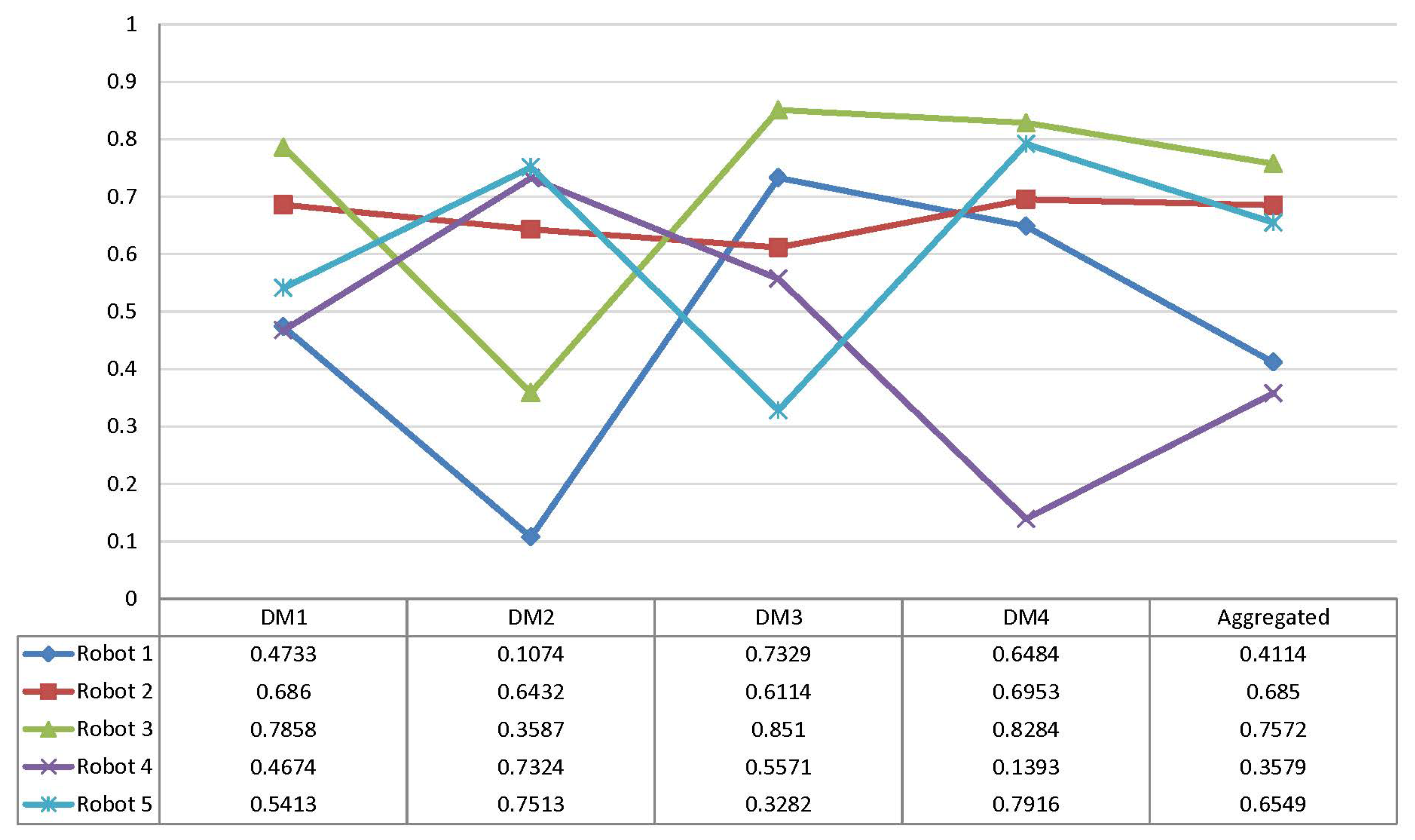
7.1. GITrF-TOPSIS Results

The ideal separation matrix ( D + ), anti ideal separation matrix ( D ), relative closeness ( R C ) and robot ranking are presented in Table 10. Moreover, the ranking order of individual DMs and the aggregated ranking order of the GITrF-TOPSIS method are recorded in Table 11 and pictured in Figure 2.

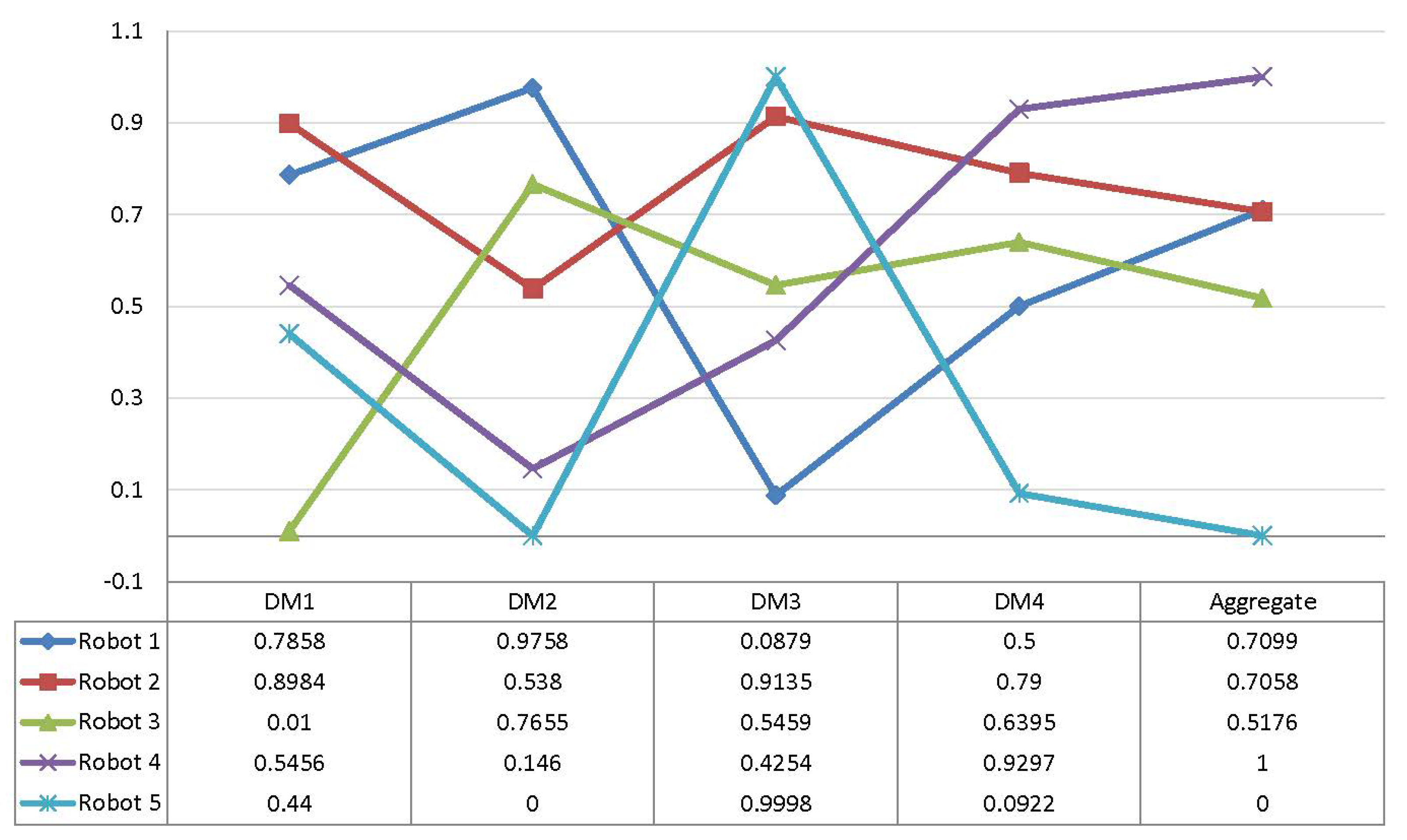
7.2. GITrF-VIKOR Results

S i , R i and Q i were calculated using Equations (21)–(23) and were recorded in Table 12. Moreover, the ranking order of individual DMs and the aggregated ranking order of the GITrF-VIKOR method were recorded in Table 13 and pictured in Figure 3.

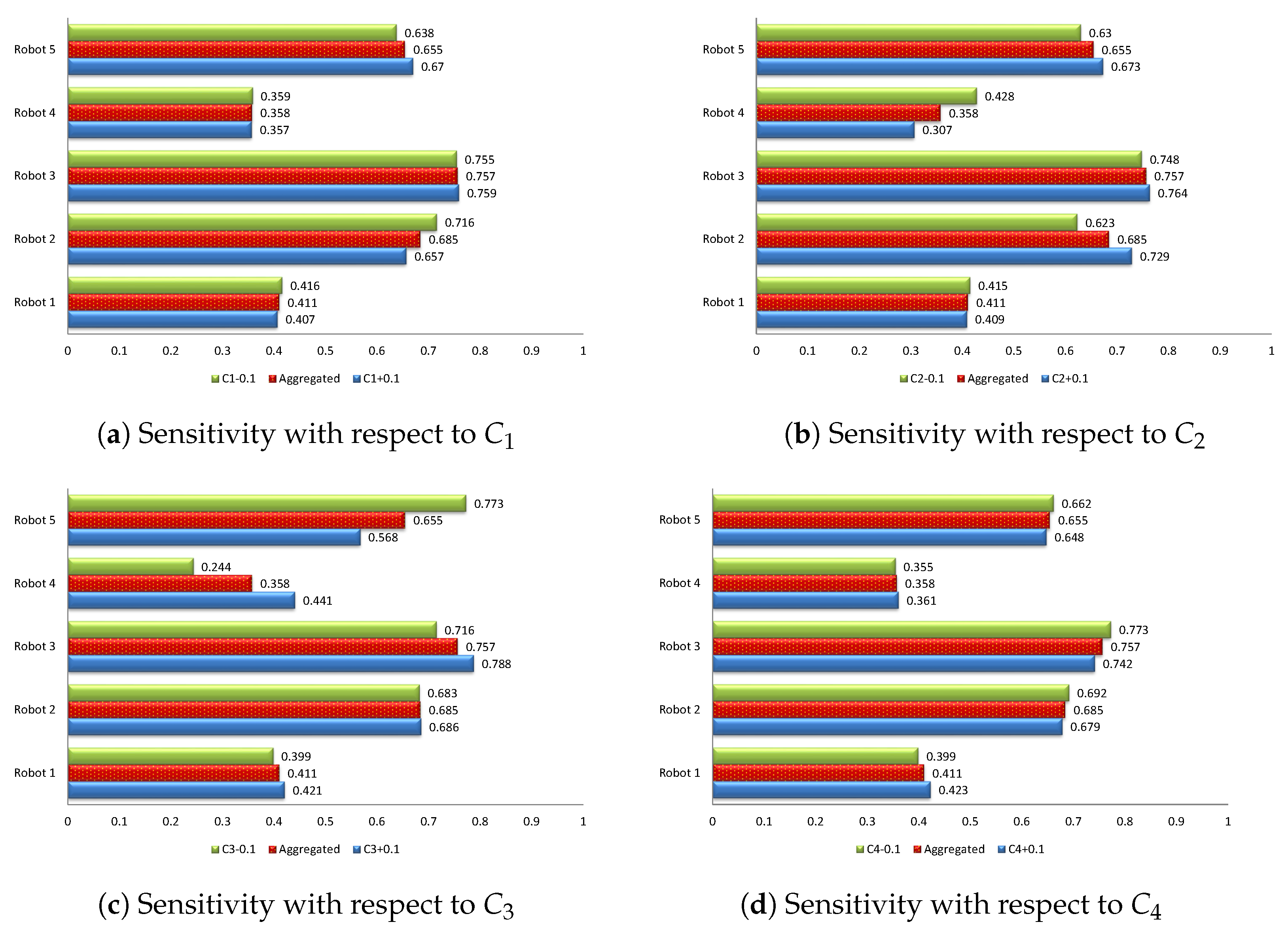
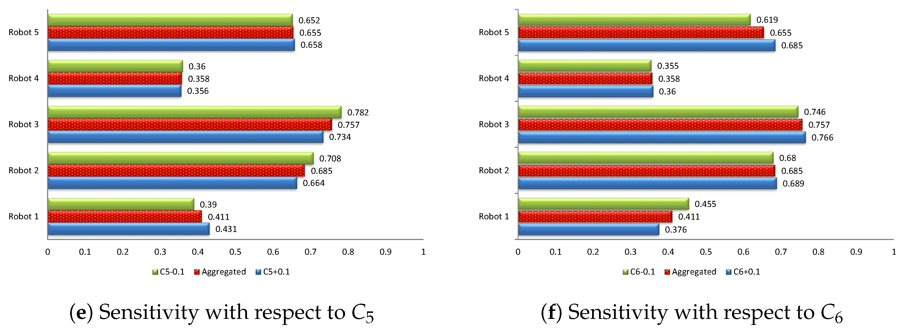
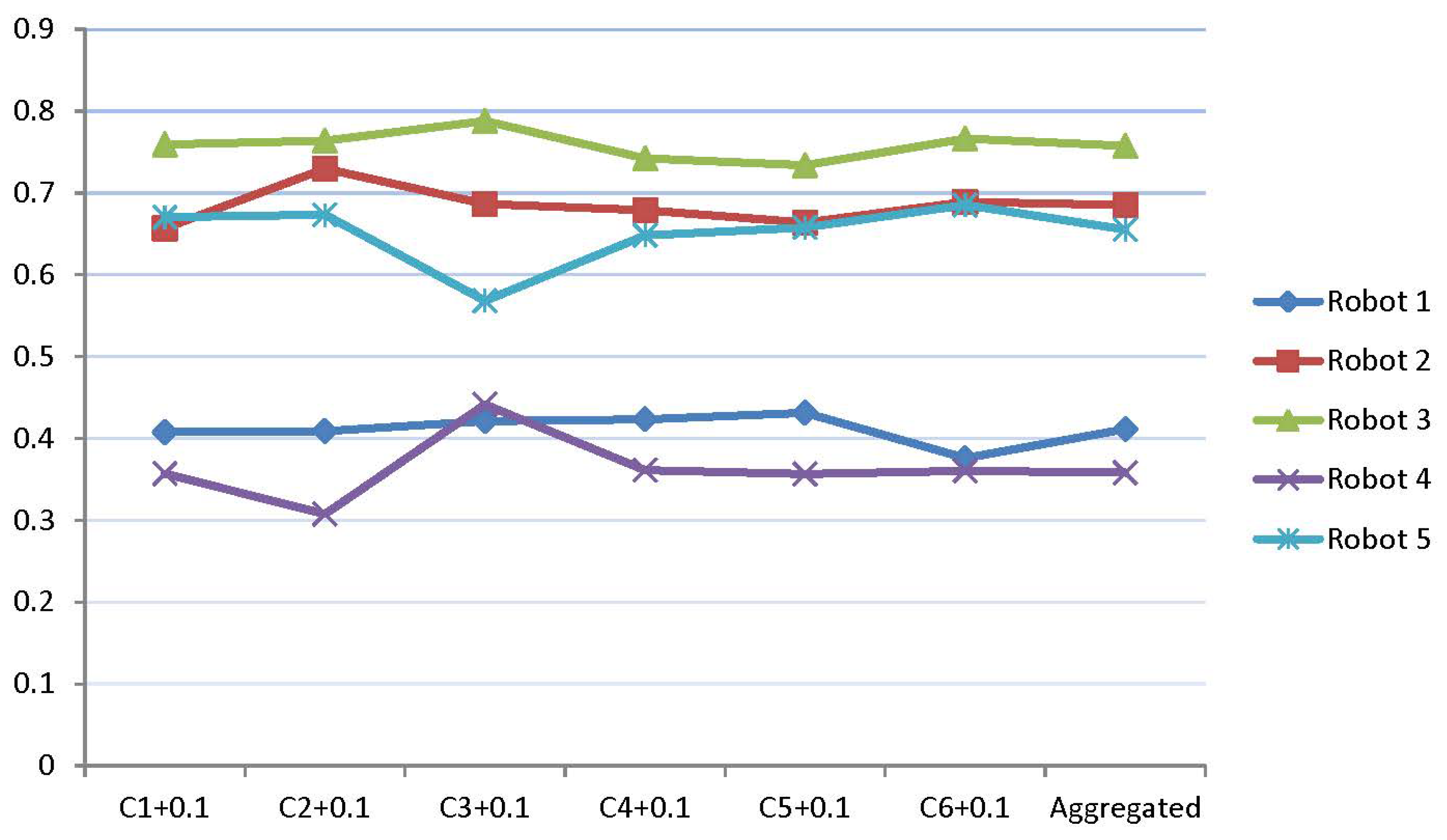
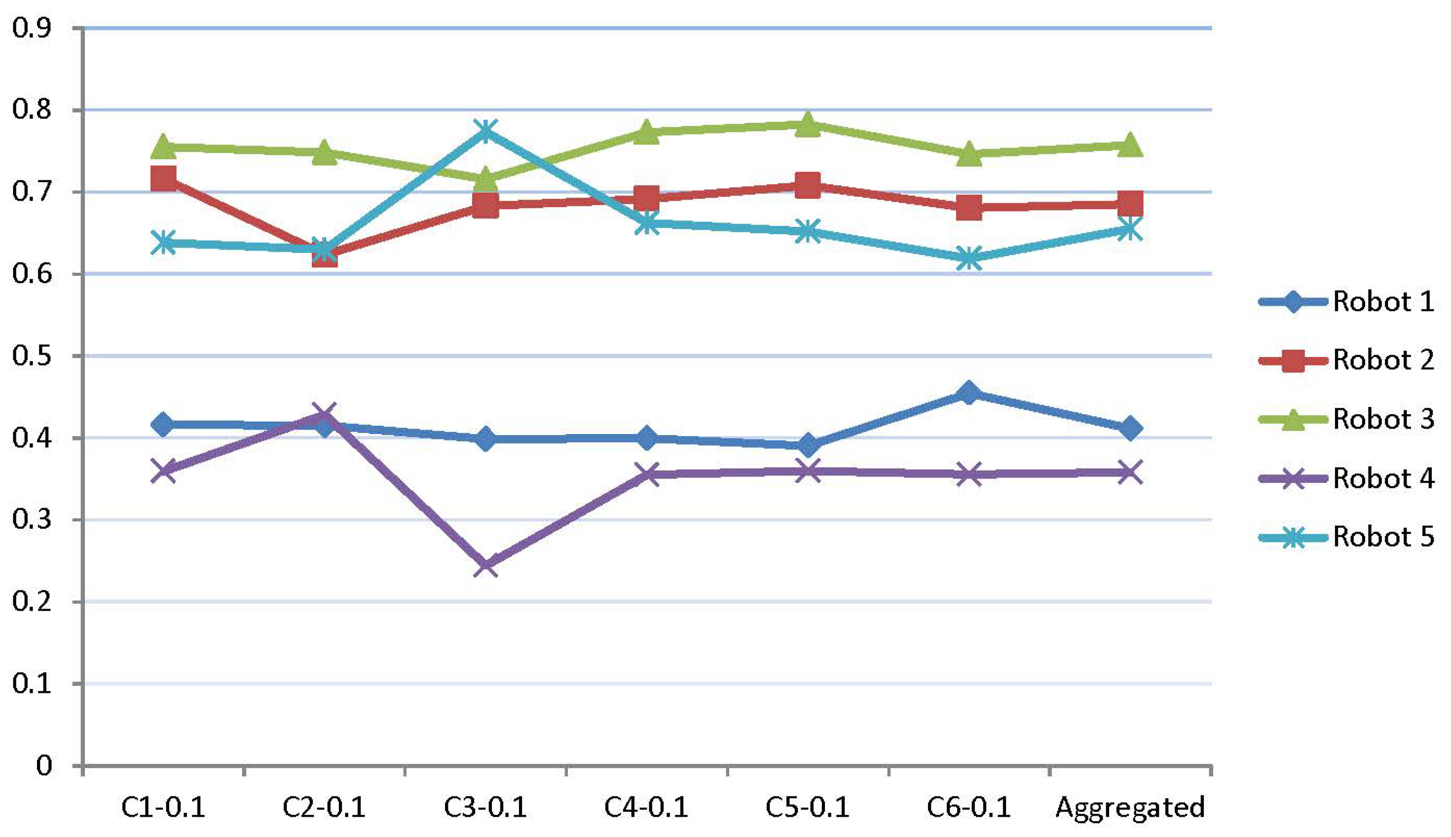
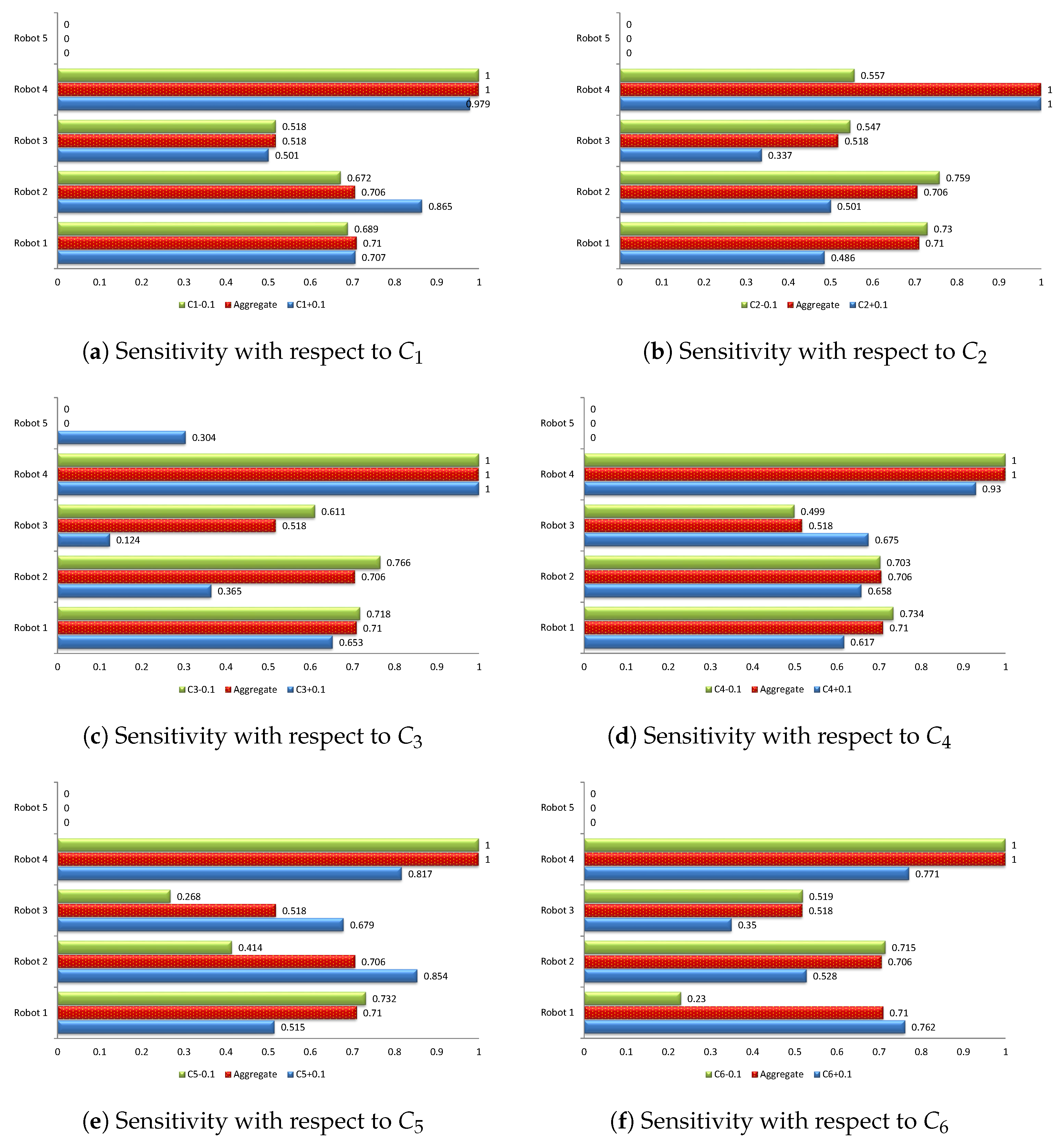
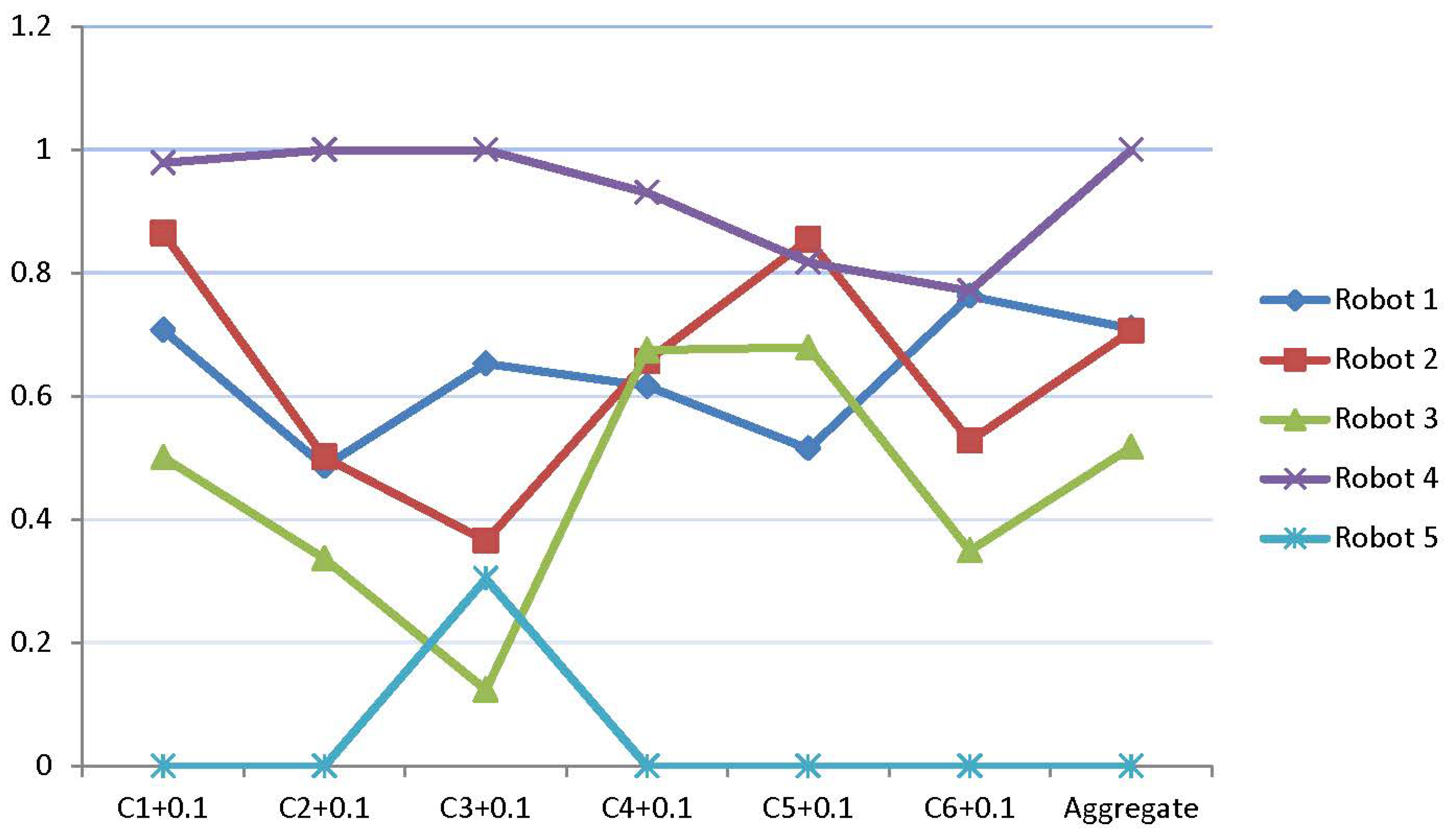
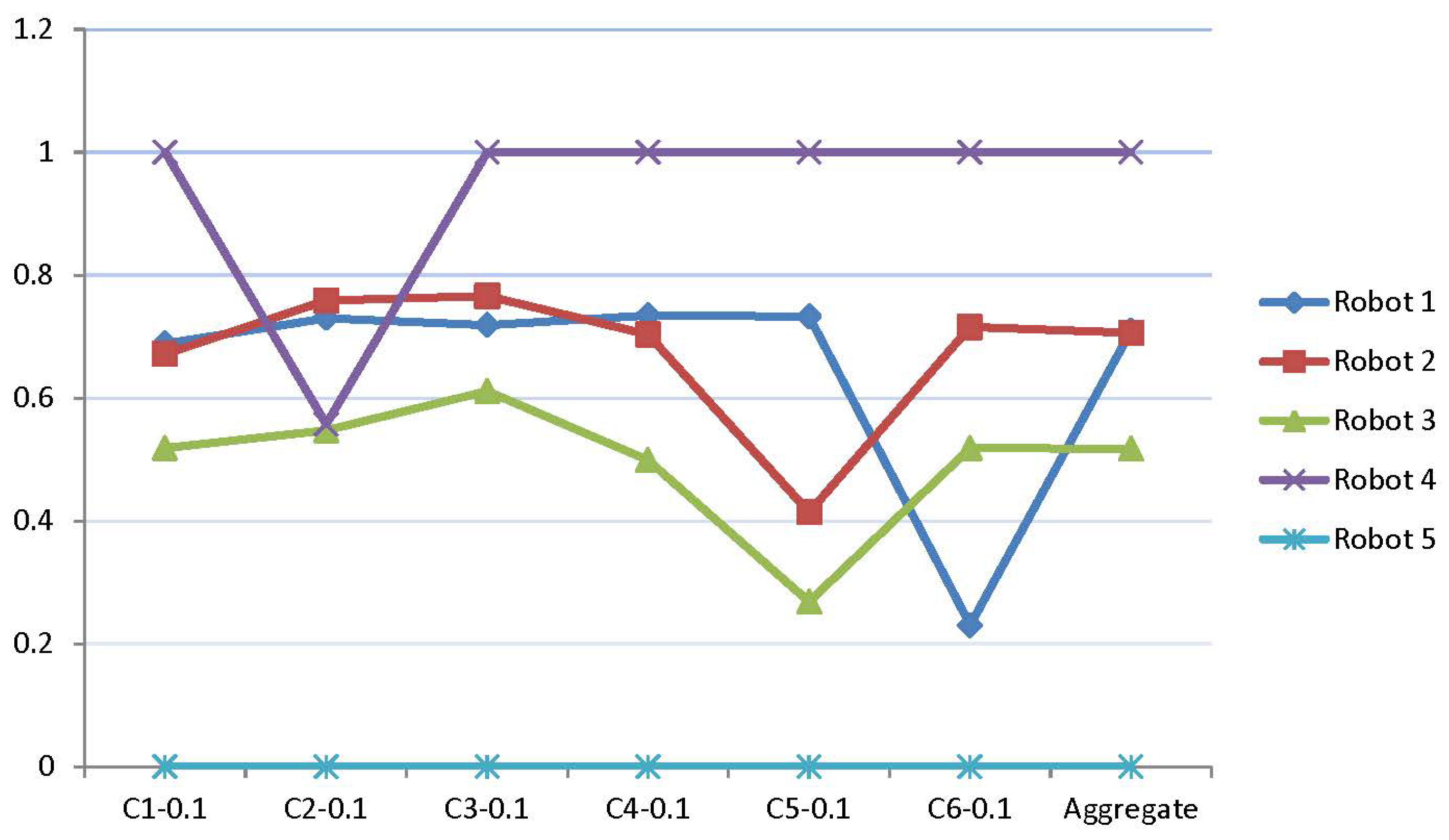
8. Sensitivity Analysis

Sensitivity analysis was performed to test how the ranking order of an MCDM method is sensitive to the variation of the weights of criteria. Sensitivity analysis was performed first by adding 0.1 to each criterion and then subtracting 0.1 from each criterion separately and adjusting other criteria accordingly to test the results with little variation in the weights and see the rank reversal of the two methods, i.e., GITrF-TOPSIS and GITrF-VIKOR. The six cases of sensitivity analysis of the GITrF-TOPSIS method are shown in Figure 4a–f, where the higher value determines the better alternative. Here, the deviations of values from the aggregated values are noted. The results show that GITrF-TOPSIS was more sensitive with respect to criteria c 2 and c 3 as shown in Figure 5 and Figure 6. The six cases of sensitivity analysis of the GITrF-VIKOR method are shown in Figure 7a–f, where the lower value determines the better alternative. Here, the deviations of values from the aggregated values are noted. The results show that GITrF-VIKOR was more sensitive with respect to criteria c 2 , c 3 , c 5 , and c 6 as shown in Figure 8 and Figure 9. It can be noted that the GITrF-VIKOR method provided more rank reversal behavior for small variations in criteria values, whereas the GITrF-TOPSIS method had less rank reversal in this scenario. The higher sensitivity and additional rank reversal behavior of the GITrF-VIKOR method is due to the distance formula (Equation (5)) used for the method. Thus, the overall sensitivity results show that the GITrF-TOPSIS method is more stable with respect to criteria as compared to the GITrF-VIKOR method.

9. Discussion

Industrial robot selection is a very difficult task in this competitive marketplace. For this selection process, deciding weights for criteria is an important factor to consider. GITrFBWM is a robust and more consistent MCDM method that assigns weights to the criteria based on preferences provided by the decision makers by utilizing their knowledge structures, experience, and expertise. For ranking of robots, the GITrF-TOPSIS and GITrF-VIKOR methods were used, and their results were compared. This is a group decision-making process that provides slightly different results for both methods. The MCDM/MCGDM method that provides less rank reversal for a small variation in criteria weights is called a stable method. Sensitivity analysis showed that the GITrF-TOPSIS method is more stable and reliable for this selection process. The proposed hybrid methodologies GITrFBWM-GITrF-TOPSIS and GITrFBWM-GITrF-VIKOR are general methodologies that are not only useful for this proposed problem but can be applied to many similar types of selection processes.

10. Conclusions

The classical methods almost fail to convey the vagueness and imprecision of the linguistic assessment. Linguistic terms are used to assist experts in providing their opinions and then convert these terms to GITrFNs. Robot selection MCGDM problems were discussed with regards to two hybrid methodologies: (1) GITrF-BWM with GITrF-TOPSIS and (2) GITrF-BWM with GITrF-VIKOR. GITrFWs are derived using GITrF-BWM, and the ranking of the robots was performed using these weights along with the GITrF-TOPSIS and GITrF-VIKOR methods separately. There is uncertainty and vagueness in real problems as human thinking is fuzzy, and thus such situations are modeled and handled using fuzzy set theory. In this research, GITrFNs were used to obtain more convincing and reliable results, as GITrFNs cover a wide area of uncertainty and applications. GITrF-BWM gives more consistent and reliable weights of criteria due to a lower consistency ratio that is a vital part of any MCDM problem. The ranking results for each decision maker and aggregated ranking results were presented for each methodology. Sensitivity analysis was performed to see the most critical weights for this problem. More sensitive criteria need more attention as compared to less sensitive criteria; the results show that the GITrF-TOPSIS method is more stable with respect to the criteria as compared to the GITrF-VIKOR method. Direct opinion-based decisions can be biased, and thus hybrid MCDM/MCGDM methodologies are needed. The proposed hybrid methodologies remedy biasess in decision processes. This research also classifies the sensitivity behavior of the proposed methods. These methodologies are general and can be applied to any criteria-based selection problem, and especially to solve social, economic, waste management, and engineering problems.
The proposed hybrid MCGDM methodologies can be applied to different managerial and engineering applications, for example hospital site selection, recruitment selection, project selection, etc. In the future, We will integrate GITrFBWM with other fuzzy and classical MCDM/MCGDM methods such as fuzzy EDAS, fuzzy CODAS, etc., and will conduct a comparative study and analysis for different social, economic, waste management, and engineering applications.

Author Contributions

Conceptualization, A.A., T.R., A.V. and J.L.G.G.; methodology, A.A., A.V.; validation, A.A., A.V. and T.R.; formal analysis, A.V., T.R. and J.L.G.G.; investigation, A.A., A.V.; data curation, A.A.; writing—original draft preparation, A.A., A.V.; writing—review and editing, T.R., A.V.; visualization, A.A.; supervision, T.R.; project administration, T.R. and J.L.G.G.; funding acquisition, J.L.G.G. All authors have read and agreed to the published version of the manuscript.

Funding

This paper was partial supported by the Ministerio de Ciencia, Innovación y Universidades grant number PGC2018-097198-B-I00 and Fundación Séneca. de la Región de Murcia grant number 20783/PI/18.

Institutional Review Board Statement

Not applicable.

Informed Consent Statement

Not applicable.

Data Availability Statement

Data are contained within the article.

Conflicts of Interest

The authors declare no conflict of interest.

Abbreviations

The following abbreviations are used in this manuscript:
BWMBest-worst method
COPRAS-GCOmplex PRoportional ASsessment of alternatives with Grey relations
CoGCenter of gravity
DMDecision maker
ELECTREELimination Et Choice Translating REality
FAHPAnalytic hierarchy process
GITrFNsGeneralized interval-valued trapezoidal fuzzy numbers
GITrFWsGeneralized interval-valued trapezoidal fuzzy weights
GITrF-BWMGeneralized interval-valued trapezoidal fuzzy best-worst method
GITrFPGeneralized interval-valued trapezoidal fuzzy preference
GITrF-RCGeneralized interval-valued trapezoidal fuzzy reference comparison
GITrF-PISGeneralized interval-valued trapezoidal fuzzy positive-ideal solution
GITrF-NISGeneralized interval-valued trapezoidal fuzzy negative-ideal solution
GMIRGraded mean integration representation
MCDMMulti-criteria decision making
MCGDMMultiple criteria group decision-making
TOPSISTechnique for Order Preference by Similarity to the Ideal Solution
TPOPTechnique of Precise Order Preferences
VIKORVIsekriterijumska optimizacija i KOmpromisno Resenje

References

  1. Zadeh, L. Fuzzy sets. Inf. Control 1965, 8, 338–353. [Google Scholar] [CrossRef] [Green Version]
  2. Bellman, R.; Zadeh, L. Decision-making in a fuzzy environment. Manag. Sci. 1970, 17, B141–B273. [Google Scholar] [CrossRef]
  3. Wu, P.; Liu, S.; Zhou, L.; Chen, H. A fuzzy group decision making model with trapezoidal fuzzy preference relations based on compatibility measure and COWGA operator. Appl. Intell. 2018, 48, 46–67. [Google Scholar] [CrossRef]
  4. Wu, P.; Wu, Q.; Zhou, L.; Chen, H.; Zhou, H. A consensus model for group decision making under trapezoidal fuzzy numbers environment. Neural Comput. Appl. 2019, 31, 377–394. [Google Scholar] [CrossRef]
  5. Wu, P.; Zhou, L.; Zheng, T.; Chen, H. A fuzzy group decision making and its application based on compatibility with multiplicative trapezoidal fuzzy preference relations. Int. J. Fuzzy Syst. 2017, 19, 683–701. [Google Scholar] [CrossRef]
  6. Luo, M.; Long, H. Picture Fuzzy Geometric Aggregation Operators Based on a Trapezoidal Fuzzy Number and Its Application. Symmetry 2021, 13, 119. [Google Scholar] [CrossRef]
  7. Wei, S.H.; Chen, S.M. Fuzzy risk analysis based on interval-valued fuzzy numbers. Expert Syst. Appl. 2009, 36, 2285–2299. [Google Scholar] [CrossRef]
  8. Chen, S.H. Ranking fuzzy numbers with maximizing set and minimizing set. Fuzzy Sets Syst. 1985, 17, 113–129. [Google Scholar] [CrossRef]
  9. Wei, S.H.; Chen, S.M. A new similarity measure between interval-valued trapezoidal fuzzy numbers based on geometric distance and the center-of-gravity-points. In Proceedings of the IEEE 2007 International Conference on Machine Learning and Cybernetics, Hong Kong, China, 19–22 August 2007; Volume 3, pp. 1412–1417. [Google Scholar]
  10. Liu, P. A weighted aggregation operators multi-attribute group decision-making method based on interval-valued trapezoidal fuzzy numbers. Expert Syst. Appl. 2011, 38, 1053–1060. [Google Scholar] [CrossRef]
  11. Liu, P.; Jin, F. A multi-attribute group decision-making method based on weighted geometric aggregation operators of interval-valued trapezoidal fuzzy numbers. Appl. Math. Model. 2012, 36, 2498–2509. [Google Scholar] [CrossRef]
  12. Ebrahimnejad, A. A simplified new approach for solving fuzzy transportation problems with generalized trapezoidal fuzzy numbers. Appl. Soft Comput. 2014, 19, 171–176. [Google Scholar] [CrossRef]
  13. Sulaiman, T.; Bulut, H.; Baskonus, H. On the exact solutions to some system of complex nonlinear models. Appl. Math. Nonlinear Sci. 2020, 6, 29–42. [Google Scholar] [CrossRef]
  14. Yu, J. A Model Study Based on Social Network Relational Dimensions and Structural Dimensions. Appl. Math. Nonlinear Sci. 2020, 5, 121–128. [Google Scholar] [CrossRef]
  15. Alghamd, M.; Alshaery, A. Mathematical Algorithm for Solving Two–Body Problem. Appl. Math. Nonlinear Sci. 2020, 5, 217–228. [Google Scholar] [CrossRef]
  16. Li, R.; Sun, T. Assessing factors for designing a successful B2C E–Commerce website using fuzzy AHP and TOPSIS–Grey methodology. Symmetry 2020, 12, 363. [Google Scholar] [CrossRef] [Green Version]
  17. de Assis, R.; Pazim, R.; Malavazi, M.; Petry, P.d.C.; de Assis, L.; Venturino, E. A mathematical model to describe the herd behaviour considering group defense. Appl. Math. Nonlinear Sci. 2020, 5, 11–24. [Google Scholar] [CrossRef] [Green Version]
  18. Zhu, P.; Fan, Q.; Zhu, J. Empirical Analysis on Environmental Regulation Performance Measurement in Manufacturing Industry: A Case Study of Chongqing, China. Appl. Math. Nonlinear Sci. 2020, 5, 25–34. [Google Scholar] [CrossRef]
  19. İnce, N.; Shamilov, A. An application of new method to obtain probability density function of solution of stochastic differential equations. Appl. Math. Nonlinear Sci. 2020, 5, 337–348. [Google Scholar] [CrossRef]
  20. Çitil, H. Important notes for a fuzzy boundary value problem. Appl. Math. Nonlinear Sci. 2019, 4, 305–314. [Google Scholar] [CrossRef] [Green Version]
  21. Ruiz-Fernández, J.P.; Benlloch Marco, J.; López, M.A.; Valverde-Gascueña, N. Influence of seasonal factors in the earned value of construction. Appl. Math. Nonlinear Sci. 2019, 4, 21–34. [Google Scholar] [CrossRef] [Green Version]
  22. Rashid, T.; Beg, I.; Husnine, S. Robot selection by using generalized interval-valued fuzzy numbers with TOPSIS. Appl. Soft Comput. 2014, 21, 462–468. [Google Scholar] [CrossRef]
  23. Ali, A.; Rashid, T. Best–worst method for robot selection. Soft Comput. 2021, 25, 563–583. [Google Scholar] [CrossRef]
  24. Rashid, T.; Ali, A.; Chu, Y.M. Hybrid BW-EDAS MCDM methodology for optimal industrial robot selection. PLoS ONE 2021, 16, e0246738. [Google Scholar] [CrossRef]
  25. Opricovic, S. Multicriteria optimization of civil engineering systems. Fac. Civ. Eng. Belgrade 1998, 2, 5–21. [Google Scholar]
  26. Athawale, V.; Chatterjee, P.; Chakraborty, S. Selection of industrial robots using compromise ranking method. Int. J. Ind. Syst. Eng. 2012, 11, 3–15. [Google Scholar] [CrossRef]
  27. Chatterjee, P.; Athawale, V.; Chakraborty, S. Selection of industrial robots using compromise ranking and outranking methods. Robot. Comput.-Integr. Manuf. 2010, 26, 483–489. [Google Scholar] [CrossRef]
  28. Devi, K. Extension of VIKOR method in intuitionistic fuzzy environment for robot selection. Expert Syst. Appl. 2011, 38, 14163–14168. [Google Scholar] [CrossRef]
  29. Rao, R.; Patel, B.; Parnichkun, M. Industrial robot selection using a novel decision making method considering objective and subjective preferences. Robot. Auton. Syst. 2011, 59, 367–375. [Google Scholar] [CrossRef]
  30. İç, Y.T.; Yurdakul, M.; Dengiz, B. Development of a decision support system for robot selection. Robot. Comput.-Integr. Manuf. 2013, 29, 142–157. [Google Scholar]
  31. Bairagi, B.; Dey, B.; Sarkar, B.; Sanyal, S. Selection of robot for automated foundry operations using fuzzy multi-criteria decision making approaches. Int. J. Manag. Sci. Eng. Manag. 2014, 9, 221–232. [Google Scholar] [CrossRef]
  32. Liu, H.C.; Ren, M.L.; Wu, J.; Lin, Q.L. An interval 2-tuple linguistic MCDM method for robot evaluation and selection. Int. J. Prod. Res. 2014, 52, 2867–2880. [Google Scholar] [CrossRef]
  33. Lanbaran, N.; Celik, E.; Yigider, M. Evaluation of investment opportunities with interval–valued fuzzy TOPSIS method. Appl. Math. Nonlinear Sci. 2020, 5, 461–474. [Google Scholar] [CrossRef]
  34. Parameshwaran, R.; Kumar, S.; Saravanakumar, K. An integrated fuzzy MCDM based approach for robot selection considering objective and subjective criteria. Appl. Soft Comput. 2015, 26, 31–41. [Google Scholar] [CrossRef]
  35. Bairagi, B.; Dey, B.; Sarkar, B.; Sanyal, S. A De Novo multi-approaches multi-criteria decision making technique with an application in performance evaluation of material handling device. Comput. Ind. Eng. 2015, 87, 267–282. [Google Scholar] [CrossRef]
  36. Samantra, C.; Datta, S.; Mahapatra, S. Selection of industrial robot using interval–valued trapezoidal fuzzy numbers set combined with VIKOR method. Int. J. Technol. Intell. Plan. 2011, 7, 344–360. [Google Scholar] [CrossRef]
  37. Ghorabaee, M. Developing an MCDM method for robot selection with interval type-2 fuzzy sets. Robot. Comput.-Integr. Manuf. 2016, 37, 221–232. [Google Scholar] [CrossRef]
  38. Jiang, L.; Zhang, T.; Feng, Y. Identifying the Critical Factors of Sustainable Manufacturing Using the Fuzzy DEMATEL Method. Appl. Math. Nonlinear Sci. 2020, 5, 391–404. [Google Scholar] [CrossRef]
  39. Joshi, D.; Kumar, S. Interval-valued intuitionistic hesitant fuzzy Choquet integral based TOPSIS method for multi-criteria group decision making. Eur. J. Oper. Res. 2016, 248, 183–191. [Google Scholar] [CrossRef]
  40. Ziemba, P.; Becker, A.; Becker, J. A consensus measure of expert judgment in the fuzzy TOPSIS method. Symmetry 2020, 12, 204. [Google Scholar] [CrossRef] [Green Version]
  41. Wang, C.N.; Dang, T.T.; Tibo, H.; Duong, D.H. Assessing renewable energy production capabilities using DEA window and fuzzy TOPSIS model. Symmetry 2021, 13, 334. [Google Scholar] [CrossRef]
  42. Moslem, S.; Farooq, D.; Ghorbanzadeh, O.; Blaschke, T. Application of the AHP–BWM Model for evaluating driver behavior factors related to road safety: A case study for Budapest. Symmetry 2020, 12, 243. [Google Scholar] [CrossRef] [Green Version]
  43. Li, T.; Yang, W. Supply Chain Planning Problem Considering Customer Inventory Holding Cost Based on an Improved Tabu Search Algorithm. Appl. Math. Nonlinear Sci. 2020, 5, 557–564. [Google Scholar] [CrossRef]
  44. Sunarsih, S.; Pamurti, R.; Khabibah, S.; Hadiyanto, H. Analysis of Priority Scale for Watershed Reforestation Using Trapezoidal Fuzzy VIKOR Method: A Case Study in Semarang, Central Java Indonesia. Symmetry 2020, 12, 507. [Google Scholar] [CrossRef] [Green Version]
  45. Khan, M.; Kumam, P.; Alreshidi, N.; Shaheen, N.; Kumam, W.; Shah, Z.; Thounthong, P. The Renewable Energy Source Selection by Remoteness Index-Based VIKOR Method for Generalized Intuitionistic Fuzzy Soft Sets. Symmetry 2020, 12, 977. [Google Scholar] [CrossRef]
  46. Sałabun, W.; Wątróbski, J.; Shekhovtsov, A. Are MCDA Methods Benchmarkable? A Comparative Study of TOPSIS, VIKOR, COPRAS, and PROMETHEE II Methods. Symmetry 2020, 12, 1549. [Google Scholar] [CrossRef]
  47. Chen, T.Y. Signed distance-based TOPSIS method for multiple criteria decision analysis based on generalized interval-valued fuzzy numbers. Int. J. Inf. Technol. Decis. Mak. 2011, 10, 1131–1159. [Google Scholar] [CrossRef]
  48. Chen, S.; Hsieh, C. Representation, ranking, distance, and similarity of LR type fuzzy number and application. Aust. J. Intell. Process. Syst. 2000, 6, 217–229. [Google Scholar]
  49. Liao, M.; Liang, G.H.; Chen, C.Y. Fuzzy grey relation method for multiple criteria decision-making problems. Qual. Quant. 2013, 47, 3065–3077. [Google Scholar] [CrossRef]
  50. Zhao, H.; Guo, S. Selecting green supplier of thermal power equipment by using a hybrid MCDM method for sustainability. Sustainability 2014, 6, 217–235. [Google Scholar] [CrossRef] [Green Version]
  51. Baležentis, T.; Zeng, S. Group multi-criteria decision making based upon interval-valued fuzzy numbers: An extension of the MULTIMOORA method. Expert Syst. Appl. 2013, 40, 543–550. [Google Scholar] [CrossRef]
  52. Ali, A.; Rashid, T. Generalized interval-valued trapezoidal fuzzy best-worst multiple criteria decision-making method with applications. J. Intell. Fuzzy Syst. 2020, 38, 1705–1719. [Google Scholar] [CrossRef]
  53. Rezaei, J. Best-worst multi-criteria decision-making method. Omega 2015, 53, 49–57. [Google Scholar] [CrossRef]
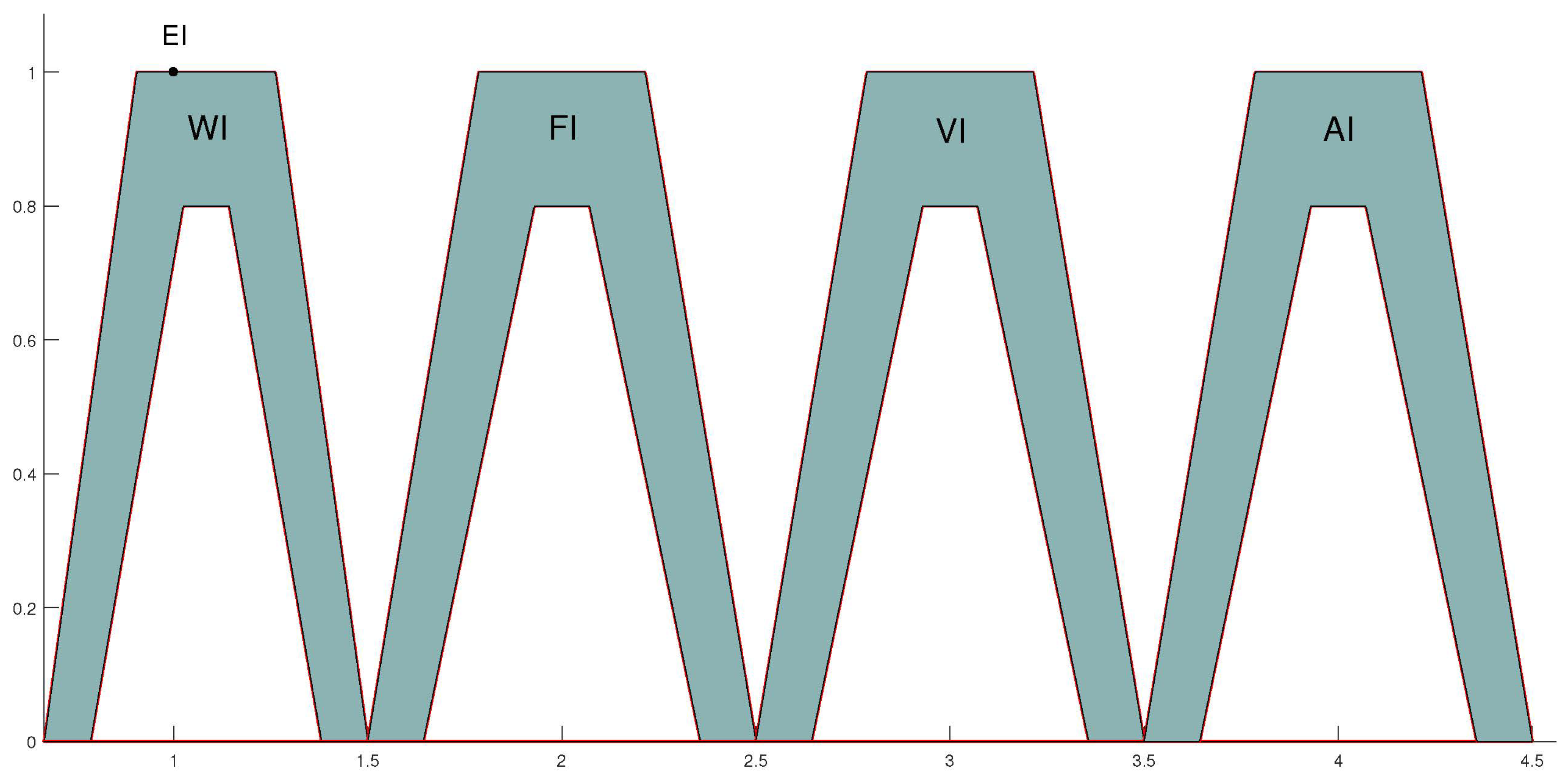
Figure 1. Graphical representation of fuzzy evaluation table for GITrF-BWM.
Symmetry 13 00839 g001
Figure 2. Decision makers’ ranking and aggregated ranking of robots using the GITrF-TOPSIS method.
Symmetry 13 00839 g002
Figure 3. Decision makers’ ranking and aggregated ranking of robots using the GITrF-VIKOR method.
Symmetry 13 00839 g003
Figure 4. Sensitivity analysis with respect to criteria for the GITrF-TOPSIS method.
Symmetry 13 00839 g004aSymmetry 13 00839 g004b
Figure 5. Sensitivity analysis of the GITrF-TOPSIS method by increased weights.
Symmetry 13 00839 g005
Figure 6. Sensitivity analysis of the GITrF-TOPSIS method by decreased weights.
Symmetry 13 00839 g006
Figure 7. Sensitivity analysis with respect to criteria for the GITrF-VIKOR method.
Symmetry 13 00839 g007
Figure 8. Sensitivity analysis of the GITrF-VIKOR method by increased weights.
Symmetry 13 00839 g008
Figure 9. Sensitivity analysis of the GITrF-VIKOR method by decreased weights.
Symmetry 13 00839 g009
Table 1. Transformation of decision makers’ linguistic terms to GITrFNs [52].
GITrFNs TransformationLinguistic Terms
[ ( 1 , 1 , 1 , 1 ; 1 ) , ( 1 , 1 , 1 , 1 ; 1 ) ] Equally Important (EI)
[ ( 0.7857 , 1.0238 , 1.1429 , 1.381 ; 0.8 ) , ( 0.6667 , 0.9048 , 1.2619 , 1.5 ; 1 ) ] Weakly Important (WI)
[ ( 1.6429 , 1.9286 , 2.0714 , 2.3571 ; 0.8 ) , ( 1.5 , 1.7857 , 2.2143 , 2.5 ; 1 ) ] Fairly Important (FI)
[ ( 2.6429 , 2.9286 , 3.0714 , 3.3571 ; 0.8 ) , ( 2.5 , 2.7857 , 3.2143 , 3.5 ; 1 ) ] Very Important (VI)
[ ( 3.6429 , 3.9286 , 4.0714 , 4.3571 ; 0.8 ) , ( 3.5 , 3.7857 , 4.2143 , 4.5 ; 1 ) ] Absolutely Important (AI)
Table 2. The rules of preference conversion of linguistic terms to GITrFNs, according to Chen [47].
GITrFNsLinguistic Terms
[ ( 0.0 , 0.0 , 0.0 , 0.0 ; 1.0 ) , ( 0.0 , 0.0 , 0.0 , 0.0 ; 1.0 ) ] Absolutely poor (AP)
[ ( 0.0075 , 0.0075 , 0.015 , 0.0525 ; 0.8 ) , ( 0.0 , 0.0 , 0.02 , 0.07 ; 1.0 ) ] Very poor (VP)
[ ( 0.0875 , 0.12 , 0.16 , 0.1825 ; 0.8 ) , ( 0.04 , 0.10 , 0.18 , 0.23 ; 1.0 ) ] Poor (P)
[ ( 0.2325 , 0.255 , 0.325 , 0.3575 ; 0.8 ) , ( 0.17 , 0.22 , 0.36 , 0.42 ; 1.0 ) ] Medium poor (MP)
[ ( 0.4025 , 0.4525 , 0.5375 , 0.5675 ; 0.8 ) , ( 0.32 , 0.41 , 0.58 , 0.65 ; 1.0 ) ] Medium (M)
[ ( 0.65 , 0.6725 , 0.7575 , 0.79 ; 0.8 ) , ( 0.58 , 0.63 , 0.80 , 0.86 ; 1.0 ) ] Medium good (MG)
[ ( 0.7825 , 0.815 , 0.885 , 0.9075 ; 0.8 ) , ( 0.72 , 0.78 , 0.92 , 0.97 ; 1.0 ) ] Good (G)
[ ( 0.9475 , 0.985 , 0.9925 , 0.9925 ; 0.8 ) , ( 0.93 , 0.98 , 1.0 , 1.0 ; 1.0 ) ] Very good (VG)
[ ( 1.0 , 1.0 , 1.0 , 1.0 ; 1.0 ) , ( 1.0 , 1.0 , 1.0 , 1.0 ; 1.0 ) ] Absolutely good (AG)
Table 3. Decision makers’ preferences for weight calculations.
DM1 p ˜ 21 p ˜ 23 p ˜ 24 p ˜ 25 p ˜ 26 p ˜ 14 p ˜ 34 p ˜ 54 p ˜ 64
WIFIAIFIWIVIFIVIVI
DM2 p ˜ 51 p ˜ 52 p ˜ 53 p ˜ 54 p ˜ 56 p ˜ 13 p ˜ 23 p ˜ 43 p ˜ 63
WIFIAIWIFIVIFIVIVI
DM3 p ˜ 12 p ˜ 13 p ˜ 14 p ˜ 15 p ˜ 16 p ˜ 26 p ˜ 36 p ˜ 46 p ˜ 56
WIWIFIFIAIVIFIFIVI
DM4 p ˜ 51 p ˜ 52 p ˜ 53 p ˜ 54 p ˜ 56 p ˜ 21 p ˜ 31 p ˜ 41 p ˜ 61
AIFIVIFIWIVIWIFIVI
Table 4. Weights of criteria and aggregated weights.
DMsWeightsGITrFNs
DM1 w 1 [ ( 0.1997 , 0.2109 , 0.2204 , 0.2417 ; 0.8 ) , ( 0.1955 , 0.2019 , 0.2332 , 0.2514 ; 1 ) ]
w 2 [ ( 0.2434 , 0.2578 , 0.2702 , 0.2950 ; 0.8 ) , ( 0.2308 , 0.2462 , 0.2857 , 0.3064 ; 1 ) ]
w 3 [ ( 0.1410 , 0.1472 , 0.1569 , 0.1769 ; 0.8 ) , ( 0.1337 , 0.1399 , 0.1684 , 0.1855 ; 1 ) ]
w 4 [ ( 0.0673 , 0.0689 , 0.0664 , 0.0779 ; 0.8 ) , ( 0.0657 , 0.0669 , 0.0789 , 0.0813 ; 1 ) ]
w 5 [ ( 0.1709 , 0.1915 , 0.2064 , 0.2394 ; 0.8 ) , ( 0.1583 , 0.1782 , 0.2241 , 0.2561 ; 1 ) ]
w 6 [ ( 0.2008 , 0.2107 , 0.2205 , 0.2419 ; 0.8 ) , ( 0.1899 , 0.2015 , 0.2332 , 0.2471 ; 1 ) ]
DM2 w 1 [ ( 0.1994 , 0.2105 , 0.2199 , 0.2410 ; 0.8 ) , ( 0.1895 , 0.2014 , 0.2327 , 0.2508 ; 1 ) ]
w 2 [ ( 0.1407 , 0.1425 , 0.1565 , 0.1770 ; 0.8 ) , ( 0.1344 , 0.1118 , 0.1679 , 0.1848 ; 1 ) ]
w 3 [ ( 0.0664 , 0.0689 , 0.0700 , 0.0776 ; 0.8 ) , ( 0.0649 , 0.0670 , 0.0742 , 0.0809 ; 1 ) ]
w 4 [ ( 0.1994 , 0.2105 , 0.2198 , 0.2368 ; 0.8 ) , ( 0.1903 , 0.2012 , 0.2343 , 0.2508 ; 1 ) ]
w 5 [ ( 0.2423 , 0.2579 , 0.2701 , 0.2946 ; 0.8 ) , ( 0.2307 , 0.2462 , 0.2858 , 0.3060 ; 1 ) ]
w 6 [ ( 0.1314 , 0.1902 , 0.2058 , 0.2387 ; 0.8 ) , ( 0.1577 , 0.1778 , 0.2241 , 0.2491 ; 1 ) ]
DM3 w 1 [ ( 0.2595 , 0.2745 , 0.2910 , 0.3306 ; 0.8 ) , ( 0.2422 , 0.2593 , 0.3161 , 0.3475 ; 1 ) ]
w 2 [ ( 0.2496 , 0.2646 , 0.2833 , 0.3282 ; 0.8 ) , ( 0.2297 , 0.2476 , 0.3126 , 0.3444 ; 1 ) ]
w 3 [ ( 0.2024 , 0.2101 , 0.2222 , 0.2553 ; 0.8 ) , ( 0.1905 , 0.1996 , 0.2433 , 0.2695 ; 1 ) ]
w 4 [ ( 0.1913 , 0.2021 , 0.2135 , 0.2500 ; 0.8 ) , ( 0.1761 , 0.1952 , 0.2354 , 0.2660 ; 1 ) ]
w 5 [ ( 0.2326 , 0.2626 , 0.2808 , 0.3260 ; 0.8 ) , ( 0.2067 , 0.2385 , 0.3099 , 0.3437 ; 1 ) ]
w 6 [ ( 0.0830 , 0.0877 , 0.0909 , 0.1046 ; 0.8 ) , ( 0.0806 , 0.0841 , 0.0969 , 0.1111 ; 1 ) ]
DM4 w 1 [ ( 0.0749 , 0.0778 , 0.0803 , 0.0871 ; 0.8 ) , ( 0.0738 , 0.0758 , 0.0850 , 0.0973 ; 1 ) ]
w 2 [ ( 0.1896 , 0.2124 , 0.2297 , 0.2726 ; 0.8 ) , ( 0.1746 , 0.1970 , 0.2511 , 0.2857 ; 1 ) ]
w 3 [ ( 0.1060 , 0.1114 , 0.1152 , 0.1295 ; 0.8 ) , ( 0.1021 , 0.1069 , 0.1225 , 0.1369 ; 1 ) ]
w 4 [ ( 0.1584 , 0.1672 , 0.1802 , 0.2037 ; 0.8 ) , ( 0.1541 , 0.1590 , 0.1932 , 0.2129 ; 1 ) ]
w 5 [ ( 0.2680 , 0.2862 , 0.3008 , 0.3293 ; 0.8 ) , ( 0.2556 , 0.2722 , 0.3192 , 0.3492 ; 1 ) ]
w 6 [ ( 0.2248 , 0.2374 , 0.2488 , 0.2748 ; 0.8 ) , ( 0.2124 , 0.2253 , 0.2691 , 0.2864 ; 1 ) ]
Aggregate w 1 [ ( 0.1834 , 0.1934 , 0.2029 , 0.2251 ; 0.8 ) , ( 0.1753 , 0.1846 , 0.2168 , 0.2368 ; 1 ) ]
w 2 [ ( 0.2058 , 0.2193 , 0.2349 , 0.2682 ; 0.8 ) , ( 0.1924 , 0.2007 , 0.2543 , 0.2803 ; 1 ) ]
w 3 [ ( 0.1290 , 0.1344 , 0.1411 , 0.1598 ; 0.8 ) , ( 0.1228 , 0.1284 , 0.1521 , 0.1682 ; 1 ) ]
w 4 [ ( 0.1541 , 0.1622 , 0.1700 , 0.1921 ; 0.8 ) , ( 0.1466 , 0.1556 , 0.1855 , 0.2028 ; 1 ) ]
w 5 [ ( 0.2285 , 0.2496 , 0.2645 , 0.2973 ; 0.8 ) , ( 0.2128 , 0.2338 , 0.2848 , 0.3138 ; 1 ) ]
w 6 [ ( 0.1600 , 0.1815 , 0.1915 , 0.2150 ; 0.8 ) , ( 0.1602 , 0.1722 , 0.2058 , 0.2234 ; 1 ) ]
Table 5. Rating of robots under subjective criteria expressed in linguistic variables.
CriteriaRototsDecision Makers
D 1 D 2 D 3 D 4
C 1 R 1 MMGVG
R 2 MGMG
R 3 GMVGMG
R 4 VGVGMGP
R 5 MGMGGG
C 2 R 1 GPGMG
R 2 VGGVGG
R 3 GMVGVG
R 4 PMGGP
R 5 MGVGMGG
C 3 R 1 MMGG
R 2 GMVGMG
R 3 GGGVG
R 4 VGVGMGG
R 5 MPMGPMP
Table 6. Ratings of robots with respect to objective criteria.
CriteriaRototsRating of Criteria
C 4 R 1 [ ( 72.25 , 72.50 , 72.70 , 73.00 ; 0.8 ) , ( 72.00 , 72.25 , 73.50 , 74.00 ; 1 ) ]
R 2 [ ( 69.00 , 69.50 , 70.00 , 71.00 ; 0.8 ) , ( 68.50 , 68.80 , 71.50 , 72.00 ; 1 ) ]
R 3 [ ( 67.50 , 68.00 , 69.00 , 69.50 ; 0.8 ) , ( 67.00 , 67.30 , 70.00 , 70.30 ; 1 ) ]
R 4 [ ( 70.00 , 70.25 , 70.65 , 71.00 ; 0.8 ) , ( 69.75 , 70.00 , 71.50 , 72.00 ; 1 ]
R 5 [ ( 68.50 , 69.00 , 70.00 , 70.75 ; 0.8 ) , ( 68.00 , 68.50 , 71.25 , 72.25 ; 1 ) ]
C 5 R 1 [ ( 48.50 , 49.00 , 50.00 , 50.50 ; 0.8 ) , ( 48.00 , 48.25 , 51.00 , 52.00 ; 1 ) ]
R 2 [ ( 44.00 , 44.50 , 45.00 , 45.50 ; 0.8 ) , ( 43.50 , 43.80 , 46.00 , 46.50 ; 1 ) ]
R 3 [ ( 43.50 , 44.00 , 45.00 , 45.50 ; 0.8 ) , ( 43.00 , 43.30 , 47.00 , 47.50 ; 1 ) ]
R 4 [ ( 45.00 , 45.50 , 46.00 , 47.00 ; 0.8 ) , ( 44.50 , 45.00 , 47.50 , 48.50 ; 1 ) ]
R 5 [ ( 47.50 , 48.00 , 48.50 , 49.00 ; 0.8 ) , ( 46.50 , 47.50 , 49.25 , 50.50 ; 1 ) ]
C 6 R 1 [ ( 0.115 , 0.120 , 0.130 , 0.135 ; 0.8 ) , ( 0.100 , 0.110 , 0.140 , 0.142 ; 1 ) ]
R 2 [ ( 0.150 , 0.157 , 0.165 , 0.170 ; 0.8 ) , ( 0.140 , 0.145 , 0.180 , 0.185 ; 1 ) ]
R 3 [ ( 0.162 , 0.165 , 0.170 , 0.175 ; 0.8 ) , ( 0.155 , 0.160 , 0.185 , 0.190 ; 1 ) ]
R 4 [ ( 0.130 , 0.136 , 0.145 , 0.151 ; 0.8 ) , ( 0.120 , 0.125 , 0.155 , 0.166 ; 1 ) ]
R 5 [ ( 0.173 , 0.178 , 0.182 , 0.189 ; 0.8 ) , ( 0.168 , 0.172 , 0.190 , 0.199 ; 1 ) ]
Table 7. Normalized decision matrix.
CriteriaRobotsNormalized Rating Value of Criteria
C 1 R 1 [ ( 0.6926 , 0.7391 , 0.8067 , 0.8292 ; 0.8 ) , ( 0.6257 , 0.7049 , 0.8415 , 0.8934 ; 1 ) ]
R 2 [ ( 0.6475 , 0.6926 , 0.7773 , 0.8060 ; 0.8 ) , ( 0.5683 , 0.6503 , 0.8197 , 0.8852 ; 1 ) ]
R 3 [ ( 0.7602 , 0.7992 , 0.8668 , 0.8900 ; 0.8 ) , ( 0.6967 , 0.7650 , 0.9016 , 0.9508 ; 1 ) ]
R 4 [ ( 0.7193 , 0.7548 , 0.7930 , 0.8081 ; 0.8 ) , ( 0.6776 , 0.7350 , 0.8142 , 0.8443 ; 1 ) ]
R 5 [ ( 0.7828 , 0.8128 , 0.8975 , 0.9276 ; 0.8 ) , ( 0.7104 , 0.7705 , 0.9399 , 1.0000 ; 1 ) ]
C 2 R 1 [ ( 0.5844 , 0.6148 , 0.6821 , 0.7075 ; 0.8 ) , ( 0.5228 , 0.5812 , 0.7157 , 0.7690 ; 1 ) ]
R 2 [ ( 0.8782 , 0.9137 , 0.9530 , 0.9645 ; 0.8 ) , ( 0.8376 , 0.8934 , 0.9746 , 1.0000 ; 1 ) ]
R 3 [ ( 0.7817 , 0.8217 , 0.8648 , 0.8782 ; 0.8 ) , ( 0.7360 , 0.7995 , 0.8883 , 0.9188 ; 1 ) ]
R 4 [ ( 0.4080 , 0.4385 , 0.4981 , 0.5235 ; 0.8 ) , ( 0.3503 , 0.4086 , 0.5279 , 0.5812 ; 1 ) ]
R 5 [ ( 0.7690 , 0.7982 , 0.8610 , 0.8832 ; 0.8 ) , ( 0.7132 , 0.7665 , 0.8934 , 0.9365 ; 1 ) ]
C 3 R 1 [ ( 0.6061 , 0.6483 , 0.7276 , 0.7545 ; 0.8 ) , ( 0.5320 , 0.6087 , 0.7673 , 0.8286 ; 1 ) ]
R 2 [ ( 0.7116 , 0.7481 , 0.8114 , 0.8331 ; 0.8 ) , ( 0.6522 , 0.7161 , 0.8440 , 0.8900 ; 1 ) ]
R 3 [ ( 0.8427 , 0.8772 , 0.9329 , 0.9501 ; 0.8 ) , ( 0.7903 , 0.8491 , 0.9616 , 1.0000 ; 1 ) ]
R 4 [ ( 0.8510 , 0.8843 , 0.9277 , 0.9418 ; 0.8 ) , ( 0.8082 , 0.8619 , 0.9514 , 0.9795 ; 1 ) ]
R 5 [ ( 0.4143 , 0.4399 , 0.5115 , 0.5422 ; 0.8 ) , ( 0.3504 , 0.4041 , 0.5473 , 0.6061 ; 1 ) ]
C 4 R 1 [ ( 0.9178 , 0.9216 , 0.9241 , 0.9273 ; 0.8 ) , ( 0.9054 , 0.9116 , 0.9273 , 0.9306 ; 1 ) ]
R 2 [ ( 0.9437 , 0.9571 , 0.9640 , 0.9710 ; 0.8 ) , ( 0.9306 , 0.9371 , 0.9738 , 0.9781 ; 1 ) ]
R 3 [ ( 0.9640 , 0.9710 , 0.9853 , 0.9926 ; 0.8 ) , ( 0.9531 , 0.9571 , 0.9955 , 1.0000 ; 1 ) ]
R 4 [ ( 0.9437 , 0.9483 , 0.9537 , 0.9571 ; 0.8 ) , ( 0.9306 , 0.9371 , 0.9571 , 0.9606 ; 1 ) ]
R 5 [ ( 0.9470 , 0.9571 , 0.9710 , 0.9781 ; 0.8 ) , ( 0.9273 , 0.9404 , 0.9781 , 0.9853 ; 1 ) ]
C 5 R 1 [ ( 0.9327 , 0.9423 , 0.9615 , 0.9712 ; 0.8 ) , ( 0.9231 , 0.9279 , 0.9808 , 1.0000 ; 1 ) ]
R 2 [ ( 0.8462 , 0.8558 , 0.8654 , 0.8750 ; 0.8 ) , ( 0.8365 , 0.8423 , 0.8846 , 0.8942 ; 1 ) ]
R 3 [ ( 0.8365 , 0.8462 , 0.8654 , 0.8750 ; 0.8 ) , ( 0.8269 , 0.8327 , 0.9038 , 0.9135 ; 1 ) ]
R 4 [ ( 0.8654 , 0.8750 , 0.8846 , 0.9038 ; 0.8 ) , ( 0.8558 , 0.8654 , 0.9135 , 0.9327 ; 1 ) ]
R 5 [ ( 0.9135 , 0.9231 , 0.9327 , 0.9423 ; 0.8 ) , ( 0.8942 , 0.9135 , 0.9471 , 0.9712 ; 1 ) ]
C 6 R 1 [ ( 0.7407 , 0.7692 , 0.8333 , 0.8696 ; 0.8 ) , ( 0.7042 , 0.7143 , 0.9091 , 1.0000 ; 1 ) ]
R 2 [ ( 0.5882 , 0.6061 , 0.6369 , 0.6667 ; 0.8 ) , ( 0.5405 , 0.5556 , 0.6897 , 0.7143 ; 1 ) ]
R 3 [ ( 0.5714 , 0.5882 , 0.6061 , 0.6173 ; 0.8 ) , ( 0.5263 , 0.5405 , 0.6250 , 0.6452 ; 1 ) ]
R 4 [ ( 0.6623 , 0.6897 , 0.7353 , 0.7692 ; 0.8 ) , ( 0.6024 , 0.6452 , 0.8000 , 0.8333 ; 1 ) ]
R 5 [ ( 0.5291 , 0.5495 , 0.5618 , 0.5780 ; 0.8 ) , ( 0.5025 , 0.5263 , 0.5814 , 0.5952 ; 1 ) ]
Table 8. Weighted normalized decision matrix.
CriteriaRobotsWeighted Normalized Rating Value of Criteria
C 1 R 1 [ ( 0.1270 , 0.1430 , 0.1637 , 0.1867 ; 0.8 ) , ( 0.1097 , 0.1301 , 0.1824 , 0.2115 ; 1 ) ]
R 2 [ ( 0.1187 , 0.1340 , 0.1577 , 0.1814 ; 0.8 ) , ( 0.0996 , 0.1200 , 0.1777 , 0.2096 ; 1 ) ]
R 3 [ ( 0.1394 , 0.1546 , 0.1759 , 0.2003 ; 0.8 ) , ( 0.1221 , 0.1412 , 0.1954 , 0.2251 ; 1 ) ]
R 4 [ ( 0.1319 , 0.1460 , 0.1609 , 0.1819 ; 0.8 ) , ( 0.1187 , 0.1357 , 0.1765 , 0.1999 ; 1 ) ]
R 5 [ ( 0.1435 , 0.1572 , 0.1821 , 0.2088 ; 0.8 ) , ( 0.1245 , 0.1422 , 0.2037 , 0.2368 ; 1 ) ]
C 2 R 1 [ ( 0.1203 , 0.1349 , 0.1602 , 0.1897 ; 0.8 ) , ( 0.1006 , 0.1166 , 0.1820 , 0.2156 ; 1 ) ]
R 2 [ ( 0.1807 , 0.2004 , 0.2239 , 0.2587 ; 0.8 ) , ( 0.1611 , 0.1793 , 0.2479 , 0.2803 ; 1 ) ]
R 3 [ ( 0.1609 , 0.1802 , 0.2032 , 0.2355 ; 0.8 ) , ( 0.1416 , 0.1604 , 0.2259 , 0.2576 ; 1 ) ]
R 4 [ ( 0.0840 , 0.0962 , 0.1170 , 0.1404 ; 0.8 ) , ( 0.0674 , 0.0820 , 0.1343 , 0.1629 ; 1 ) ]
R 5 [ ( 0.1583 , 0.1751 , 0.2023 , 0.2369 ; 0.8 ) , ( 0.1372 , 0.1538 , 0.2272 , 0.2625 ; 1 ) ]
C 3 R 1 [ ( 0.0782 , 0.0871 , 0.1026 , 0.1206 ; 0.8 ) , ( 0.0653 , 0.0781 , 0.1167 , 0.1394 ; 1 ) ]
R 2 [ ( 0.0918 , 0.1005 , 0.1145 , 0.1332 ; 0.8 ) , ( 0.0801 , 0.0919 , 0.1284 , 0.1497 ; 1 ) ]
R 3 [ ( 0.1087 , 0.1179 , 0.1316 , 0.1519 ; 0.8 ) , ( 0.0970 , 0.1090 , 0.1463 , 0.1682 ; 1 ) ]
R 4 [ ( 0.1097 , 0.1188 , 0.1309 , 0.1505 ; 0.8 ) , ( 0.0992 , 0.1106 , 0.1447 , 0.1648 ; 1 ) ]
R 5 [ ( 0.0534 , 0.0591 , 0.0722 , 0.0867 ; 0.8 ) , ( 0.0430 , 0.0519 , 0.0832 , 0.1020 ; 1 ) ]
C 4 R 1 [ ( 0.1414 , 0.1495 , 0.1571 , 0.1781 ; 0.8 ) , ( 0.1327 , 0.1418 , 0.1720 , 0.1887 ; 1 ) ]
R 2 [ ( 0.1454 , 0.1552 , 0.1639 , 0.1865 ; 0.8 ) , ( 0.1364 , 0.1458 , 0.1806 , 0.1983 ; 1 ) ]
R 3 [ ( 0.1486 , 0.1575 , 0.1675 , 0.1907 ; 0.8 ) , ( 0.1397 , 0.1489 , 0.1846 , 0.2028 ; 1 ) ]
R 4 [ ( 0.1454 , 0.1538 , 0.1621 , 0.1839 ; 0.8 ) , ( 0.1364 , 0.1458 , 0.1775 , 0.1948 ; 1 ) ]
R 5 [ ( 0.1459 , 0.1552 , 0.1650 , 0.1879 ; 0.8 ) , ( 0.1359 , 0.1463 , 0.1814 , 0.1998 ; 1 ) ]
C 5 R 1 [ ( 0.2131 , 0.2352 , 0.2544 , 0.2887 ; 0.8 ) , ( 0.1965 , 0.2169 , 0.2793 , 0.3138 ; 1 ) ]
R 2 [ ( 0.1933 , 0.2136 , 0.2289 , 0.2602 ; 0.8 ) , ( 0.1780 , 0.1969 , 0.2519 , 0.2806 ; 1 ) ]
R 3 [ ( 0.1911 , 0.2112 , 0.2289 , 0.2602 ; 0.8 ) , ( 0.1760 , 0.1947 , 0.2574 , 0.2866 ; 1 ) ]
R 4 [ ( 0.1977 , 0.2184 , 0.2340 , 0.2687 ; 0.8 ) , ( 0.1821 , 0.2023 , 0.2601 , 0.2926 ; 1 ) ]
R 5 [ ( 0.2087 , 0.2304 , 0.2467 , 0.2802 ; 0.8 ) , ( 0.1903 , 0.2135 , 0.2697 , 0.3047 ; 1 ) ]
C 6 R 1 [ ( 0.1185 , 0.1396 , 0.1596 , 0.1870 ; 0.8 ) , ( 0.1128 , 0.1230 , 0.1871 , 0.2234 ; 1 ) ]
R 2 [ ( 0.0941 , 0.1100 , 0.1220 , 0.1433 ; 0.8 ) , ( 0.0866 , 0.0957 , 0.1419 , 0.1596 ; 1 ) ]
R 3 [ ( 0.0914 , 0.1068 , 0.1161 , 0.1327 ; 0.8 ) , ( 0.0843 , 0.0931 , 0.1286 , 0.1441 ; 1 ) ]
R 4 [ ( 0.1060 , 0.1252 , 0.1408 , 0.1654 ; 0.8 ) , ( 0.0965 , 0.1111 , 0.1647 , 0.1862 ; 1 ) ]
R 5 [ ( 0.0847 , 0.0997 , 0.1076 , 0.1243 ; 0.8 ) , ( 0.0805 , 0.0906 , 0.1197 , 0.1330 ; 1 ) ]
Table 9. GITrF-PIS and GITrF-NIS for criteria.
CriteriaGITrF-PIS/GITrF-NISNormalized Rating Value of Criteria
C 1 GITrF-PIS [ ( 0.1435 , 0.1572 , 0.1821 , 0.2088 ; 0.8 ) , ( 0.1245 , 0.1422 , 0.2037 , 0.2368 ; 1 ) ]
GITrF-NIS [ ( 0.1187 , 0.1340 , 0.1577 , 0.1814 ; 0.8 ) , ( 0.0996 , 0.1200 , 0.1765 , 0.1999 ; 1 ) ]
C 2 GITrF-PIS [ ( 0.1807 , 0.2004 , 0.2239 , 0.2587 ; 0.8 ) , ( 0.1611 , 0.1793 , 0.2479 , 0.2803 ; 1 ) ]
GITrF-NIS [ ( 0.0840 , 0.0962 , 0.1170 , 0.1404 ; 0.8 ) , ( 0.0674 , 0.0820 , 0.1343 , 0.1629 ; 1 ) ]
C 3 GITrF-PIS [ ( 0.1097 , 0.1188 , 0.1316 , 0.1519 ; 0.8 ) , ( 0.0992 , 0.1106 , 0.1463 , 0.1682 ; 1 ) ]
GITrF-NIS [ ( 0.0534 , 0.0591 , 0.0722 , 0.0867 ; 0.8 ) , ( 0.0430 , 0.0519 , 0.0832 , 0.1020 ; 1 ) ]
C 4 GITrF-PIS [ ( 0.1414 , 0.1495 , 0.1571 , 0.1781 ; 0.8 ) , ( 0.1327 , 0.1418 , 0.1720 , 0.1887 ; 1 ) ]
GITrF-NIS [ ( 0.1486 , 0.1575 , 0.1675 , 0.1907 ; 0.8 ) , ( 0.1397 , 0.1489 , 0.1846 , 0.2028 ; 1 ) ]
C 5 GITrF-PIS [ ( 0.2131 , 0.2352 , 0.2544 , 0.2887 ; 0.8 ) , ( 0.1965 , 0.2169 , 0.2793 , 0.3138 ; 1 ) ]
GITrF-NIS [ ( 0.1911 , 0.2112 , 0.2289 , 0.2602 ; 0.8 ) , ( 0.1760 , 0.1947 , 0.2519 , 0.2806 ; 1 ) ]
C 6 GITrF-PIS [ ( 0.0847 , 0.0997 , 0.1076 , 0.1243 ; 0.8 ) , ( 0.0805 , 0.0906 , 0.1197 , 0.1330 ; 1 ) ]
GITrF-NIS [ ( 0.1185 , 0.1396 , 0.1596 , 0.1870 ; 0.8 ) , ( 0.1128 , 0.1230 , 0.1871 , 0.2234 ; 1 ) ]
Table 10. D + , D , R C and ranking of the GITrF-TOPSIS method.
D + D RC Ranking
0.14850.10380.41144
0.07950.17280.68502
0.06130.19110.75721
0.16200.09030.35795
0.08710.16530.65493
Table 11. Ranking results of the GITrF-TOPSIS method.
GITrF-TOPSIS Ranking
DM1 R 3 R 2 R 5 R 1 R 4
DM2 R 5 R 4 R 2 R 3 R 1
DM3 R 3 R 1 R 2 R 4 R 5
DM4 R 3 R 5 R 2 R 1 R 4
Aggregated R 3 R 2 R 5 R 1 R 4
Table 12. S i , R i , Q i and ranking of the GITrF-VIKOR method.
S i R i Q i Ranking
0.47600.17490.70994
0.53010.16930.70583
0.43810.16890.51762
0.61300.176115
0.35780.150501
Table 13. Ranking results of the GITrF-VIKOR method.
GITrF-VIKOR Ranking
DM1 R 3 R 5 R 4 R 1 R 2
DM2 R 5 R 4 R 2 R 3 R 1
DM3 R 1 R 4 R 3 R 2 R 5
DM4 R 5 R 1 R 3 R 2 R 4
Aggregated R 5 R 3 R 2 R 1 R 4
Publisher’s Note: MDPI stays neutral with regard to jurisdictional claims in published maps and institutional affiliations.

