Abstract
The emergence of the COVID-19 outbreak has caused a pandemic situation in over 210 countries. Controlling the spread of this disease has proven difficult despite several resources employed. Millions of hospitalizations and deaths have been observed, with thousands of cases occurring daily with many measures in place. Due to the complex nature of COVID-19, we proposed a system of time-fractional equations to better understand the transmission of the disease. Non-locality in the model has made fractional differential equations appropriate for modeling. Solving these types of models is computationally demanding. Our proposed generalized compartmental COVID-19 model incorporates effective contact rate, transition rate, quarantine rate, disease-induced death rate, natural death rate, natural recovery rate, and recovery rate of quarantine infected for a holistic study of the coronavirus disease. A detailed analysis of the proposed model is carried out, including the existence and uniqueness of solutions, local and global stability analysis of the disease-free equilibrium (symmetry), and sensitivity analysis. Furthermore, numerical solutions of the proposed model are obtained with the generalized Adam–Bashforth–Moulton method developed for the fractional-order model. Our analysis and solutions profile show that each of these incorporated parameters is very important in controlling the spread of COVID-19. Based on the results with different fractional-order, we observe that there seems to be a third or even fourth wave of the spike in cases of COVID-19, which is currently occurring in many countries.
1. Introduction
In 2019, the COVID-19 outbreak was sudden and rapidly spreading beyond understanding at the time, with more than 213 countries declaring the disease as a pandemic. The coronavirus disease, formally known as COVID-19 or SARS-CoV-2, originated in the city of Wuhan, in the Hubei province of China. The source is still unknown. It is believed that an animal reservoir caused the appearance of the virus in the human population. In recent times, many countries have started an investigation into the exact source of this new coronavirus. COVID-19 has spawned a global pandemic that has substantially affected millions around the world. The coronavirus disease causes an upper-respiratory infection that is easily transmitted between hosts with no known vaccine. The Centers for Disease Control and Prevention have declared this outbreak a public health risk. This disease spreads through droplets caused by coughs, sneezes, or talking within a range of approximately six feet. It is known that social distancing and face masks are effective ways to prevent the spread of the virus between hosts. COVID-19 has affected people all over the world and continues to spread. Throughout history, major pandemics have occurred, such as the Spanish Flu (1981–1920) and the recent Ebola epidemic (2014–2016), that have had a significant impact on human health and global economics. As for recently (March 2021), the coronavirus has infected more than 127.3 million people worldwide, killing over 2.7 million people. Specifically, in the USA, over 31 million cases have already been recorded, with over 540,000 deaths [1].
The importance of modeling and tracking the severity of the virus is not only necessary to prepare for future outbreaks, but to inform governments and citizens of what they should be doing now to mitigate transmission and infection. By modeling and tracking the trend of the current outbreak, we can prepare for outbreaks in the upcoming seasons. Doing this will help reduce the severity of next coronavirus outbreaks. There have been many proposed mathematical models and analyses by a large number of infectious disease researchers on COVID-19 and similar diseases see [2,3,4,5,6,7,8,9,10,11]. Furthermore, some authors have proposed a SIR or related models for COVID-19. In [3,5,6], the Susceptible-Exposed-Infected-Recovered (SEIR) model was used to analyze data generated from Italy and China. Furthermore, in [8], Anastassopouloua et al. used the Susceptible-Infected-Recovered-Dead (SIRD) model to calculate the basic reproduction number, infection, and per day recovery rate for the data generated from China. Recent approaches in dealing with infectious diseases such as COVID-19 using data-driven methods such as machine learning and deep learning, hybrid artificial intelligence, and principal component analysis can be found in [12,13,14,15,16,17]. However, COVID-19 is rare, complex, and many things are yet unknown, which set limitations to what known models (especially the integer-order models) could capture.
Non-integer (fractional) order derivatives can be used to model most phenomena in science, engineering, and social science. This is due to the property of non-locality, which is inherent in many complex structures. Some example applications are seen in biological modeling, financial modeling, and random walk, dynamical system control theory, viscoelasticity, nanotechnology, anomalous transport, and anomalous diffusion [18,19,20,21,22,23,24,25,26,27,28]. It should be noted here that solving fractional differential equations is very difficult due to the memory effect. Beyond numerical methods, which are often computationally demanding, different analytical methods have been proposed to handle linear and nonlinear fractional differential equations, see [19,29,30,31,32,33,34,35,36].
Due to the complex nature of COVID-19, this paper explores the use of fractional calculus to develop mathematical models in order to understand and answer the following pertinent questions: (1) what parameters are essential (most impactful) for control measure purposes; (2) dynamics of the spread and long time impact of the disease in different population densities; and (3) what to expect at the resurgence of the outbreak and necessary control measures to reduce the impact. This work is focused on advancing research to understand better factors that could help curtailing, or possible control measures for eradication for a long time benefit. Different control measures are investigated using effective, efficient, and more general mathematical models to reveal the intrinsic nature of the COVID-19. Modeling, analysis, and numerical solutions are the focus of the current paper on the disease transmission and spread that includes understanding the delay to ’flattening the curve’ as experienced in many cities and countries.
Specifically, our proposed generalized compartmental COVID-19 model takes into account many key parameters to gain insight into the complexity of the disease. The parameters considered are effective contact rate, transition rate (from exposed quarantine and recovered to susceptible and infected quarantined individuals), quarantine rate, disease-induced death rate, natural death rate, natural recovery rate, and recovery rate of quarantine infected. We simulate and discuss the parameters on the dynamics of the solution profiles. In this paper, a detailed analysis of the proposed model is carried out, including the existence and uniqueness of solutions, local and global stability analysis, endemic equilibrium analysis, and sensitivity analysis. In addition, numerical solutions of the proposed fractional SEQIR model are obtained using the generalized Adam–Bashforth–Moulton method developed for the fractional-order model.
The rest of the paper is structured as follows: In Section 2, preliminaries are presented to include basic definitions, notations used in this present investigation, and valuable results from the literature. The generalized mathematical model is formulated in Section 3, which accounts for the loss of immunity of the infected recovered individuals. Analysis of the model to include the existence and uniqueness of solutions, local and global stability analysis, endemic equilibrium (symmetry) analysis, and sensitivity analysis is presented with detailed proofs in Section 4. The numerical simulation of the proposed model is presented in Section 5. Finally, Section 6 is devoted to summary and recommendations.
2. Preliminaries
In this section, we present some definitions, notations, and some known results needed in sequel. Caputo’s fractional derivative is adopted in this work.
Definition 1.
A real valued function u is said to be in the space , , , if there exists a real number p with such that
where , and it is said to be in the space iff , .
Definition 2.
The Laplace transform is defined by
where is an n-dimensional vector-valued function.
Definition 3.
The Riemann–Liouville’s fractional integral operator of order , of a function is given as
where Γ is the Gamma function, and .
Definition 4.
The fractional derivative in the Caputo’s sense is defined as [37],
where , , .
Lemma 1.
Let . Then
Definition 5.
The generalized Mittag–Leffler function (also called two-parameter Mittag–Leffler function) is defined as:
When , a special case of this function is obtained, called a one-parameter Mittag–Leffler function, given as:
Taking different values for and , we see that this function represents many important special cases, such as:
The generalized Mittag–Leffler function is an entire function [38,39], so bounded in any finite interval.
Lemma 2.
[40] Let , and . Then, the function , is positive monotonically decreasing functions of .
Definition 6.
Let . Then, the Laplace transform of the Caputo’s fractional derivative is given as
where .
Lemma 3.
Considering the two-parameter Mittag–Leffler function, the Laplace transform formula is given as
where , , .
Lemma 4.
[41] For , let and . Then
Lemma 4 is called the generalized mean value theorem.
3. Model Formulation
In this section, we develop a compartmental COVID-19 model where individuals are classified at time t as: susceptible (S), exposed (E), exposed but quarantined (), infected (I), infected but quarantined (), and recovered (R). The infected compartment, contains both asymptomatic and symptomatic carriers who have not been clinically confirmed to be COVID-19 positive. Transmission of COVID-19 occurs as a result of touching a contaminated surface or sharing very close space (less than 6 ft/2m) with an infectious host coughing or sneezing [42]. We assume that exposed and infected individuals are able to transmit the disease to the general public, but quarantined individuals, either exposed or infected, are unable to transmit the virus to general public because they stay in isolation. Susceptible individuals contract the disease at a rate Once individuals are confirmed positive, they are placed in self-quarantine (or hospitalize) at rate We incorporate the parameters for quarantine rate of exposed individuals, progression rate from exposure to infected class, and progression rate from exposed quarantined to infected quarantined class, respectively. Individuals in I and decrease by diseased-induced death rate There are several reports that recovered individuals are susceptible to re-infection. On 24 April 2020, the World Health Organization (WHO) reported that there is currently no proof that individuals who have recovered from COVID-19 and have tested negative for the virus are immune to re-infection [1]. Because of this, we take into consideration loss of immunity at rate See Figure 1 for an illustration of the model and Table 1 for the model parameters.
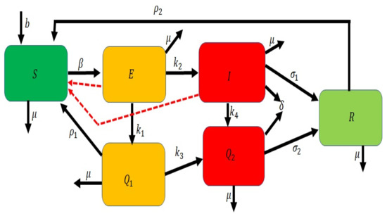
Figure 1.
A schematic diagram of the model.

Table 1.
Parameters of the disease model and their meanings.
A nonlinear system under the above transmission assumptions is given by
and initial points to be
with , the Caputo fractional derivative of order . The parameters are birth, per capital death rates of individuals, natural recovery rate, recovery rate of quarantine infected, and transition rate from recovered to susceptible individuals, respectively. All the parameters are defined and values provided in Table 1 below. Note that This means that
4. Analysis of the Time-Fractional COVID-19 Model
Our focus in this Section is on detailed analysis of the proposed COVID-19 model of time-fractional type. The existence, uniqueness, and non-negativity results of solutions to the system (10)–(11) are presented and proven. We further investigate conditions and results on existence, stability (local and global), and equilibrium of the proposed model.
The region is an area which contains all biologically and mathematically relevant solutions of system (10)–(11).
We denote the following parameter for easy calculation.
4.1. Results on the Existence and Uniqueness Of Solutions
The following Lemma is needed to prove the existence and uniqueness of solutions to the system considered in (10)–(11). Our results include the forward-invariant property of the domain considered.
Lemma 5.
For , let and . Then
- (a)
- the function u is non-decreasing if , .
- (b)
- the function u is non-increasing if , .
Proof.
The proof is a direct consequence of Lemma 4. □
Theorem 1.
Proof.
Using Theorem (3.1) and Remark (3.2) in [49], the existence and uniqueness of the solution in is obtained. Furthermore, we need to show that the closed set ∇ is forward-invariant w.r.t (10). To prove this, we first consider the fractional differential:
Using the Laplace transform given in 6 in both sides, we obtain
Re-arranging (12), we get
Applying Laplace inverse transform, and Lemma 3 after some simplification, we obtain the solution as
Recall that
Using (14) combined with Lemma 2, it follows that
Thus, ∇ is positive and bounded. So, all solutions of the system (10) and (11) are confined in the set ∇. □
4.2. Existence, Stability, and Equilibrium Results for COVID-19 Model of Fractional Type
From above, the region ∇ is positively-invariant under models (10) and (11). Then the system is both epidemiologically and mathematically well-posed. Therefore, it is sufficient to study the dynamics of the model in ∇.
In the absence of COVID-19, we have and at equilibrium
There exists a disease-free equilibrium of system (10) given by
4.2.1. Computation of
The basic reproduction number of infectious disease models, denoted by , is a critical epidemiological quantity of public health concerns. It measures the intensity of an outbreak of diseases and plays a significant role in evaluating control strategies. We will use a method called next generation described in [50,51,52] to compute of our model. This method is defined as the largest eigenvalue of the matrix , where the matrices F and are determined as follows:
and
Therefore
and
where
The basic reproduction number () is the spectral radius of and is given by
4.2.2. Stability Results
Theorem 2
(Local Stability). The disease-free equilibrium of system (10) is locally asymptotically stable if , and unstable if .
Proof.
To determine the local stability of the disease-free equilibrium, we use the eigenvalues of the associated Jacobian matrix. The Jacobian matrix of system (3) at
is
The characteristic equation of the Jacobian matrix is
where
For all the roots of the characteristic equation have negative real parts. □
The public health implication of Theorem 2 is that the spread of the virus can be reduced or controlled when if the initial sizes of the sub-populations of the model are in the basin of attraction of the DFE (∇). Global stability of the is necessary to ensure that the disease elimination is independent of the initial sizes of the sub-populations [53].
Theorem 3
(Global Stability). The disease-free equilibrium of system 10 is globally asymptotically stable if .
Proof.
Consider the Lyapunov function defined as
Then
We have when and when provided that It follows from the the generalized Lasalle invariance principle [54] that the disease-free equilibrium is globally asymptotically stable. □
4.2.3. Computation of an Endemic Equilibrium
Next, we summarize the predictions of endemic equilibrium of model 10 in the following Lemma.
Lemma 6 (Equilibrium).
Let
4.2.4. Sensitivity Analysis
In this subsection, we perform sensitivity analysis to determine which model parameters have the most significant impact on the threshold and the spread of the virus. When designing control strategies, sensitivity analysis can help identify parameters that should be controlled. We compute a sensitive index for the model parameters; the index predicts the relative change in for the relative change in the parameters [55,56,57]. The parameters have a positive impact on the meaning that an increase in these parameters implies an increase in , while the have negative impact on (decrease) the
Definition 7.
The normalized forward sensitivity index of a variable, L, that depends differentially on a parameter, y, is defined as:
The sensitivity indices with respect to the model parameters are as follows.
It is important to note that a sensitive index can be a constant or depend on other parameters of the model. An implies that increasing or decreasing y by a given percentage always increases (decreases) by that same percentage [58].
Based on Equation (24) and the sensitivity indices in Table 2, the most influential parameters are We make the following recommendations.
- Quarantining infected people may be an essential prevention measure to reduce the spread of COVID-19 infection.
- Reducing the transmission parameter is essential in reducing the transmission of the infection. To reduce the transmission parameter, compliance with protocols such as social distancing, wearing a face mask, and washing hands are necessary.
5. Numerical Analysis and Simulation
For completeness, we present in this Section the basic idea behind the method of solution employed to obtain solutions to the proposed system of time fractional model for COVID-19 given in (10).
5.1. Adams–Bashforth–Moulton Method for Fractional-Order
Adams–Bashforth–Moulton Method has been applied to integer order differential equations for many years. Here, we give brief description of this method applied to fractional-order differential equations. We refer the readers to see [59,60,61] for detailed results on stability and convergence. Given the initial valued fractional differential system of the form
and the initial condition
with , , and , are given constants which are real numbers. Define the Volterra integral equation as
Any continuous solution to the initial value fractional differential system (26) is also a solution of the Volterra integral equation given in (27) and vice versa. With the assumption of uniform grid with , , , is the step size, we give Adams–Bashforth–Moulton method of fractional-order type. We further assume that we first computed the approximation , then find the approximation using (27). The derivation for the case of the one-step Adams–Bashforth–Moulton scheme is similar to the approach used here with some modification making use of the Volterra integral equation in (27). This is a Predictor–Corrector method. The main idea for the corrector is to approximate the integral term in (27) with product trapezoidal quadrature formula with nodes , . To get the predictor for this case, product rectangle rule is employed. Define
and
Then, the Adams–Bashforth–Moulton Method for fractional-order type which solves system (26) is given as follows:
R. Roberto in [62] developed MATLAB subroutine for the implementation of the above method in MATLAB code fde12. With slight modification, we have employed the MATLAB function fde12 for numerical simulation of our proposed time-fractional COVID-19 model given in (26).
5.2. Numerical Simulation and Analysis
Our numerical simulations of the proposed COVID-19 model of time-fractional type are presented here with various analysis. The values of parameters used are as given in Table 1 unless otherwise stated. Effects of the fractional-order in the dynamics of the solution profiles obtained for various variables are investigated with meaningful observations. This is an important aspect of our study since the study of the nature and dynamics of COVID-19 (spread, resurgence etc.) is still ongoing, and not much is yet known. These intrinsic properties of COVID-19 could be captured using fractional derivative in time compared with integer order. Furthermore, we simulate with different values of fractional-order with different values of key parameters. The effects of these key parameters are expedient as well be able to tell what measure is effective in handling the spread of the disease and for crucial decisions given different values of fractional-orders as well.
5.2.1. Impact of Time-Fractional-Order on the Solution Profiles for the COVID-19 Model
The proposed COVID-19 model is simulated for different fractional-order values , using the baseline values of the parameters provided in Table 1. Figure 2a represents the solution of susceptible individuals , Figure 2b represents the solution of exposed individuals , Figure 2c represents the solution of exposed but quarantined individuals , Figure 2d represents the solution of infected individuals , Figure 2e represents the solution of infected but quarantined individuals , and Figure 2f represents the solution of recovered individuals . As shown in Figure 2a–f, the intrinsic properties of the fractional-orders are unique; the solution curves display delays in the epidemic peak for different fractional-order and flatten faster. For smaller values, the impact is more pronounced. From a public health perspective, this observation is vital, as hospitalization would not be overloaded due to the flattening of the curve. Although the number of infected individuals decreases dramatically for smaller fractional-orders, the number of susceptible individuals increases, compare Figure 2a,d for .
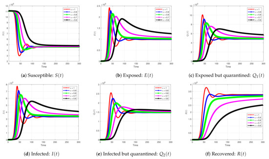
Figure 2.
The dynamics of the proposed model with different .
5.2.2. Impact of the Effective Contact Rate on the Solution Profiles for the Coivd-19 Model
We investigated the contributions of the effective contact rate on the propagation of the COVID-19. We set the fractional-order as , and varied the . The dynamics of our proposed model for the different values of the transmission parameter are displayed in Figure 3a–f, Figure 4a–f, Figure 5a–f and Figure 6a–f, respectively. As the transmission parameter rises, the infected individuals attain a higher peak level, Figure 3d,e, Figure 4d,e, Figure 5d,e, and Figure 6d,e. These effects are consistent with the sensitivity analysis result that shows the influence of the effective contact rate.
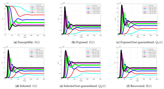
Figure 3.
with different .
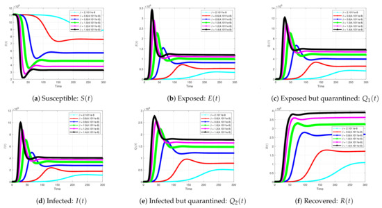
Figure 4.
with different .
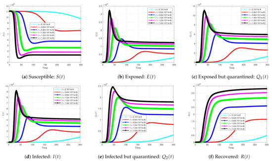
Figure 5.
with different .
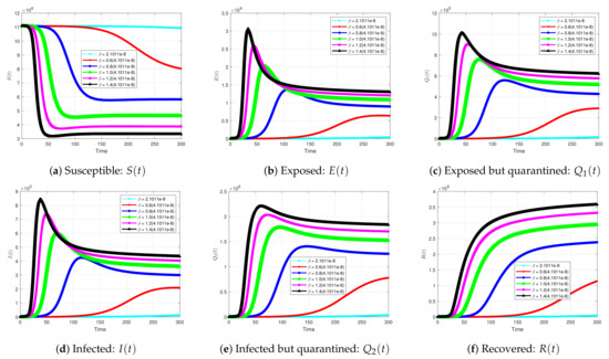
Figure 6.
with different .
5.2.3. Impact of Quarantining Exposed Individuals on the Solution Profiles for the Coivd-19 Model
We ran simulations of the model to access the population-level impact of quarantining on the outbreak. The simulations results are displayed in Figure 7a–f, for The results for , , are given in Figure 8a–f, Figure 9a–f and Figure 10a–f, respectively. The results show that quarantining exposed individuals reduces the number of infected individuals. For example, the default scenario result, with , shows a projected 800,000 cases at the peak time (Figure 7a). Without quarantining, about 1,400,000 cases will be recorded at the peak time. This result is approximately a increment of cases. A increase in quarantine baseline value results in approximately a 25% (600,000) reduction in infected cases, Figure 7a. Similarly, with the default value , the projected peak daily infected cases was 700,000 observed for , 625,000 cases reached for , and 600,000 cases attained for A increase in quarantining rate from the baseline value results in about 20–25% reduction of infected cases, Figure 8d, Figure 9d and Figure 10d.
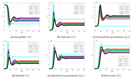
Figure 7.
with different .
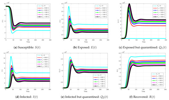
Figure 8.
with different .
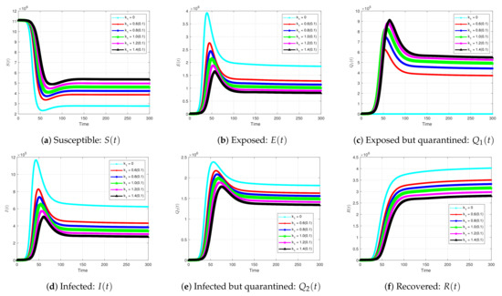
Figure 9.
with different .
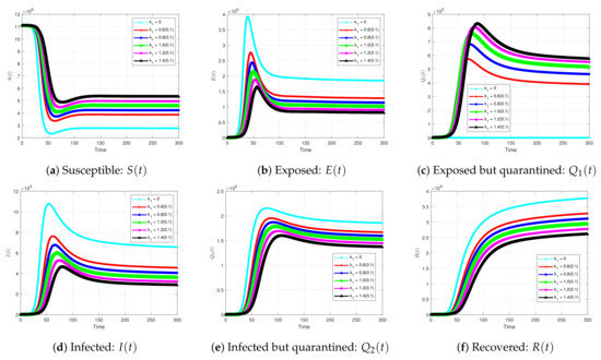
Figure 10.
with different .
5.2.4. The Impact of the Loss of Immunity
There are several reports of re-infection of the COVID-19 cases. We simulated and investigated the impacts of transition rate from recovered to susceptible individuals (loss of immunity) on the dynamics of the solution profiles. The results are displayed in Figure 11a–f, Figure 12a–f, Figure 13a–f, and Figure 14a–f. We observed that loss of immunity increases the number of infected cases. Without it, the number of individuals in the recovered compartment rises.
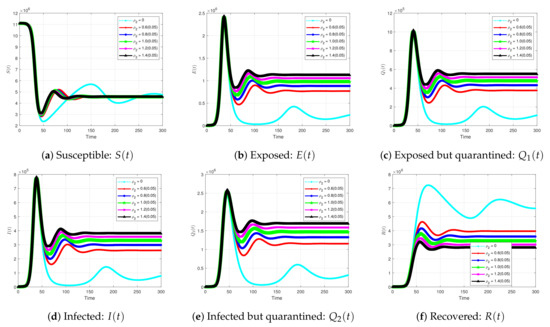
Figure 11.
with different .
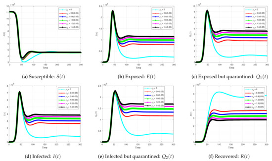
Figure 12.
with different .
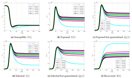
Figure 13.
with different .
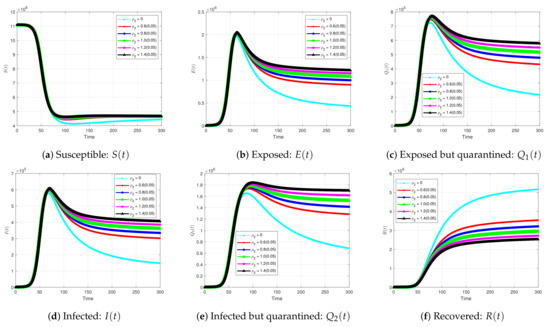
Figure 14.
with different .
5.2.5. The Impact of Quarantine Infected Individuals on the Solution Profiles for the Coivd-19 Model
The impact of quarantining infected individuals was also investigated. The simulation results for different are given in Figure 15a–f for , Figure 16a–f for , Figure 17a–f, for , and Figure 18a–f for . The results indicate that a high quarantining rate decreases the number of individuals in the infected (I) and exposed (E) classes. As displayed in Figure 15b,d, Figure 16b,d, and Figure 17b,d, without quarantine intervention, the exposed and infected populations grow faster with very high peak levels. In Figure 15, d, with a increase in quarantining rate from the baseline value, about 50,000 cases are observed at the peak time. Without quarantine, approximately 3,800,000 people will be infected at the peak time; thus, an over 400% increase of infected cases.
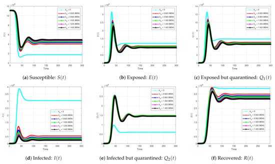
Figure 15.
with different .
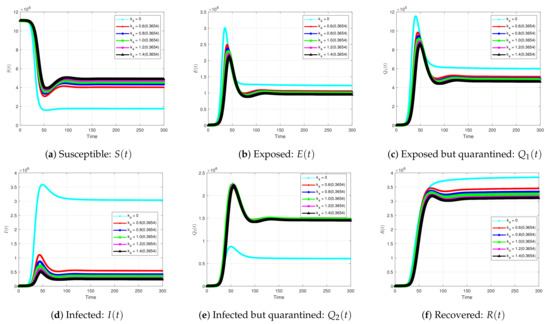
Figure 16.
with different .
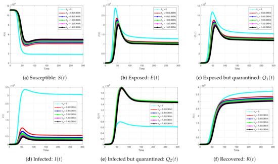
Figure 17.
with different .
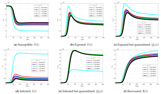
Figure 18.
with different .
6. Conclusions
The COVID-19 spread has caused many damages, and it is still posing a significant challenge to individuals and countries. Many studies have been conducted to understand the transmission dynamics and control of the outbreak. The complexity of the disease is very high, and the rate at which it spreads is alarming. Based on this, we have proposed a fractional SEQIR model that captured many intrinsic properties of the transmission of the virus (COVID-19). Deep and extensive simulations in this paper provided insights and exposed hidden properties in the transmission of the coronavirus.
The proposed generalized compartmental COVID-19 model incorporates many key parameters to gain insight into the complexity of the disease. Effective contact rate, transition rate (from exposed quarantine and recovered to susceptible and infected quarantined individuals), quarantine rate, disease-induced death rate, natural death rate, natural recovery rate, and recovery rate of quarantine infected are part of our study. We simulated and discussed the parameters on the dynamics of the solution profiles. Detailed analysis of the proposed model was done, and the results on the existence and uniqueness of solutions, local and global stability analysis of the disease-free equilibrium, and sensitivity analysis are rigorously proven. An expression for the reproduction number, the threshold that measures the contagiousness of the outbreak, was established. For a numerical solution, we employed the generalized Adam–Bashforth–Moulton method developed for the fractional-order model. The effects of the critical parameters are also discussed in detail.
Based on the results, quarantining exposed and infected individuals is sensitive and significantly impacts the transmission of the virus. Thus, the importance of quarantine in mitigating the pandemic cannot be overlooked, and an effective strategy to control the spread of the disease. The results also suggest that the effective contact parameter influences the reproduction number and the spread of the disease significantly. The results also indicate that the effective contact parameter influences the reproduction number and the spread of the disease significantly. We highly recommend using both non-pharmaceutical and pharmaceutical measures to substantially reduce the effective contact rate and minimize the transmission of the virus. New surges in waves have started to occur currently in many places globally, including the USA. Our results indicate such surges with some appropriate choice of parameters and specific fractional-order.
Author Contributions
Writing—review and editing, O.I., B.O., T.Z., B.I. and D.K. All authors contributed equally to this work which included mathematical theory and analysis and code implementation. All authors have read and agreed to the published version of the manuscript.
Funding
This research received no external funding.
Institutional Review Board Statement
Not applicable.
Informed Consent Statement
Not applicable.
Data Availability Statement
Not Applicable.
Conflicts of Interest
The authors declare no conflict of interest.
References
- World Health Organization (WHO). Available online: https://www.who.int/emergencies/diseases/novel-coronavirus-2019/media-resources/news (accessed on 19 June 2020).
- Iyiola, O.S.; Oduro, B.; Akinyemi, L. Analysis and solutions of generalized Chagas vectors re-infestation model of fractional order type. Chaos Solitons Fractals 2021, 145, 110797. [Google Scholar] [CrossRef]
- Lin, Q.; Zhao, S.; Gao, D.; Lou, Y.; Yang, S.; Musa, S.S.; Wang, M.H.; Cai, Y.; Wang, W.; Yang, L.; et al. A conceptual model for the coronavirus disease 2019 (COVID-19) outbreak in Wuhan, China with individual reaction and governmental action. Int. J. Infect. Dis. 2020, 93, 211–216. [Google Scholar] [CrossRef] [PubMed]
- Owusu-Mensah, I.; Akinyemi, L.; Oduro, B.; Iyiola, O.S. A fractional order approach to modeling and simulations of the novel COVID-19. Adv. Differ. Equ. 2020, 1, 1–21. [Google Scholar]
- Rong, X.; Yang, L.; Chu, H.; Fan, M. Effect of delay in diagnosis on transmission of COVID-19. MBE 2020, 17, 2725–2740. [Google Scholar] [CrossRef]
- Fang, Y.; Nie, Y.; Penny, M. Transmission dynamics of the COVID-19 outbreak and effectiveness of government interventions: A data-driven analysis. J. Med. Virol. 2020, 92, 645–659. [Google Scholar] [CrossRef]
- Adeniyi, M.O.; Matthew, I.E.; Iluno, C.; Ogunsanya, A.S.; Akinyemi, J.A.; Oke, S.I.; Matadi, M.B. Dynamic model of COVID-19 disease with exploratory data analysis. Sci. Afr. 2020, 9, e00477. [Google Scholar] [CrossRef]
- Anastassopoulou, C.; Russo, L.; Tsakris, A.; Siettos, C. Data-based analysis, modelling and forecasting of the COVID-19 outbreak. PLoS ONE 2020, 15, e0230405. [Google Scholar] [CrossRef]
- Oke, S.I.; Ojo, M.M.; Adeniyi, M.O.; Matadi, M.B. Mathematical modeling of malaria disease with control strategy. Commun. Math. Biol. Neurosci. 2020, 43. [Google Scholar] [CrossRef]
- Okedoye, A.M.; Salawu, S.O.; Oke, S.I.; Oladejo, N.K. Mathematical analysis of affinity hemodialysis on T-Cell depletion. Sci. Afr. 2020, 8, e00427. [Google Scholar] [CrossRef]
- Gbadamosi, B.; Ojo, M.M.; Oke, S.I.; Matadi, M.B. Qualitative analysis of a Dengue fever model. Math. Comput. Appl. 2018, 23, 33. [Google Scholar] [CrossRef]
- Gatta, V.L.; Moscato, V.; Postiglione, M.; Sperli, G. An epidemiological neural network exploiting dynamic graph structured data applied to the COVID-19 outbreak. IEEE Trans. Big Data 2021, 7, 45–55. [Google Scholar] [CrossRef]
- Ardabili, S.F.; Mosavi, A.; Ghamisi, P.; Ferdinand, F.; Varkonyi-Koczy, A.R.; Reuter, U.; Rabczuk, T.; Atkinson, P.M. COVID-19 outbreak prediction with machine learning. Algorithms 2020, 13, 249. [Google Scholar] [CrossRef]
- Pinter, G.; Felde, I.; Mosavi, A.; Ghamisi, P.; Gloaguen, R. COVID-19 pandemic prediction for Hungary; a hybrid machine learning approach. Mathematics 2020, 8, 890. [Google Scholar] [CrossRef]
- Ardabili, S.; Mosavi, A.; Band, S.S.; Varkonyi-Koczy, A.R. Coronavirus disease (COVID-19) global prediction using hybrid artificial intelligence method of ANN trained with Grey Wolf optimizer. medRxiv 2020. [Google Scholar] [CrossRef]
- Mahmoudi, M.R.; Heydari, M.H.; Qasem, S.N.; Mosavi, A.; Band, S.S.; Varkonyi-Koczy, A.R. Principal component analysis to study the relations between the spread rates of COVID-19 in high risks countries. Alex. Eng. J. 2021, 60, 457–464. [Google Scholar] [CrossRef]
- Tabrizchi, H.; Mosavi, A.; Szabo-Gali, A.; Felde, I.; Nadai, L. Rapid COVID-19 diagnosis using deep learning of the computerized tomography Scans. In Proceedings of the 2020 IEEE 3rd International Conference and Workshop in Óbuda on Electrical and Power Engineering (CANDO-EPE), Budapest, Hungary, 18–19 November 2020. [Google Scholar]
- Kumar, D.; Seadawy, A.R.; Joardar, A.K. Modified Kudryashov method via new exact solutions for some conformable fractional differential equations arising in mathematical biology. Chin. J. Phys. 2018, 56, 75–85. [Google Scholar] [CrossRef]
- Iyiola, O.S.; Zaman, F.D. A fractional diffusion equation model for cancer tumor. Am. Inst. Phys. Adv. 2014, 4, 107121. [Google Scholar] [CrossRef]
- Baleanu, D.; Wu, G.C.; Zeng, S.D. Chaos analysis and asymptotic stability of generalized Caputo fractional differential equations. Chaos Solitons Fractals 2017, 102, 99–105. [Google Scholar] [CrossRef]
- Nasrolahpour, H. A note on fractional electrodynamics. Commun. Nonlinear. Sci. Numer. Simul. 2013, 18, 2589–2593. [Google Scholar] [CrossRef]
- Hilfer, R.; Anton, L. Fractional master equations and fractal time random walks. Phys. Rev. 1995, 51, R848–R851. [Google Scholar] [CrossRef]
- Zhang, Y.; Pu, Y.F.; Hu, J.R.; Zhou, J.L. A class of fractional-order variational image in-painting models. Appl. Math. Inf. Sci. 2012, 6, 299–306. [Google Scholar]
- Pu, Y.F. Fractional differential analysis for texture of digital image. J. Alg. Comput. Technol. 2007, 1, 357–380. [Google Scholar]
- Baleanu, D.; Guvenc, Z.B.; Machado, J.T. New Trends in Nanotechnology and Fractional Calculus Applications; Springer: New York, NY, USA, 2010. [Google Scholar]
- Mainardi, F. Fractional Calculus and Waves in Linear Viscoelasticity; Imperial College Press: London, UK, 2010. [Google Scholar]
- Tarasov, V.E.; Tarasova, V.V. Time-dependent fractional dynamics with memory in quantum and economic physics. Ann. Phys. 2017, 383, 579–599. [Google Scholar] [CrossRef]
- Sun, H.G.; Zhang, Y.; Baleanu, D.; Chen, W.; Chen, Y.Q. A new collection of real world applications of fractional calculus in science and engineering. Commun. Nonlinear. Sci. Numer. Simulat. 2018, 64, 213–231. [Google Scholar] [CrossRef]
- Senol, M. Analytical and approximate solutions of (2+1)-dimensional time-fractional Burgers-Kadomtsev-Petviashvili equation. Commun. Theor. Phys. 2020, 72, 1–11. [Google Scholar] [CrossRef]
- Akinyemi, L.; Iyiola, O.S. Exact and approximate solutions of time-fractional models arising from physics via Shehu transform. Math. Methods Appl. Sci. 2020, 1–23. [Google Scholar] [CrossRef]
- Akinyemi, L.; Iyiola, O.S. A reliable technique to study nonlinear time-fractional coupled Korteweg-de Vries equations. Adv. Differ. Equ. 2020, 169, 1–27. [Google Scholar] [CrossRef]
- Akinyemi, L. q-Homotopy analysis method for solving the seventh-order time-fractional Lax’s Korteweg–de Vries and Sawada–Kotera equations. Comp. Appl. Math. 2019, 38, 1–22. [Google Scholar] [CrossRef]
- Şenol, M.; Iyiola, O.S.; Daei Kasmaei, H.; Akinyemi, L. Efficient analytical techniques for solving time-fractional nonlinear coupled Jaulent-Miodek system with energy-dependent Schrödinger potential. Adv. Differ. Equ. 2019, 2019, 1–21. [Google Scholar] [CrossRef]
- Akinyemi, L.; Iyiola, O.S.; Akpan, U. Iterative methods for solving fourth- and sixth order time-fractional Cahn-Hillard equation. Math. Methods Appl. Sci. 2020, 43, 4050–4074. [Google Scholar] [CrossRef]
- Iyiola, O.S. Exact and Approximate Solutions of Fractional Diffusion Equations with Fractional Reaction Terms. Progr. Fract. Differ. Appl. 2016, 2, 21–30. [Google Scholar] [CrossRef]
- Iyiola, O.S. On the solutions of nonlinear time-fractional gas dynamic equations: An analytical approach. Int. J. Pure Appl. Math. 2015, 98, 491–502. [Google Scholar]
- Podlubny, I. Fractional Differential Equations. In Vol. 198 of Mathematics in Science and Engineering; Academic Press: San Diego, CA, USA, 1999. [Google Scholar]
- Prabhakar, T.R. A singular integral equation with a generalized mittag-leffler function in the kernel. Yokohama Math. J. 1971, 19, 7–15. [Google Scholar]
- Iyiola, O.S.; Asante-Asamani, E.O.; Wade, B.A. A real distinct poles rational approximation of generalized Mittag–Leffler functions and their inverses: Applications to fractional calculus. J. Comput. Appl. Math. 2018, 330, 307–317. [Google Scholar] [CrossRef]
- Furati, K.M.; Iyiola, O.S.; Mustapha, K. An inverse source problem for a two-parameter anomalous diffusion with local time datum. Comput. Math. Appl. 2017, 73, 1008–1015. [Google Scholar] [CrossRef]
- Odibat, Z.M.; Shawagfeh, N.T. Generalized Taylor’s formula. Appl. Math. Comput. 2007, 186, 286–293. [Google Scholar] [CrossRef]
- World Health Organization. WHO COVID-19 Dashboard. Available online: https://who.sprinklr.com (accessed on 7 April 2020).
- Tang, B.; Bragazzi, N.L.; Li, Q.; Tang, S.; Xiao, Y.; Wu, J. An updated estimation of the risk of transmission of the novel coronavirus (2019-nCov). Infect. Dis. Model. 2020, 5, 248–255. [Google Scholar] [CrossRef]
- Lauer, S.A.; Grantz, K.H.; Bi, Q.; Jones, F.K.; Zheng, Q.; Meredith, H.R.; Lessler, J. The incubation period of coronavirus disease 2019 (COVID-19) from publicly reported confirmed cases: Estimation and application. Ann. Intern. Med. 2020, 172, 577–582. [Google Scholar] [CrossRef]
- Li, R.; Pei, S.; Chen, B.; Song, Y.; Zhang, T.; Yang, W.; Haman, J. Substantial undocumented infection facilitates the rapid dissemination of novel coronavirus (SARS-CoV2). Science 2020, 368, 489–493. [Google Scholar] [CrossRef]
- Liu, T.; Hu, J.; Kang, M.; Lin, L.; Zhong, H.; Xiao, J.; He, G.; Song, T.; Huang, Q.; Rong, Z.; et al. Transmission dynamics of 2019 novel coronavirus (2019-nCoV). bioRxiv 2020. [Google Scholar] [CrossRef]
- Zhou, F.; Yu, T.; Du, R.; Fan, G.; Liu, Y.; Liu, Z.; Guan, L. Clinical course and risk factors for mortality of adult inpatients with COVID-19 in Wuhan, China: A retrospective cohort study. Lancet 2020, 395, 1054–1062. [Google Scholar] [CrossRef]
- Huang, C.; Wang, Y.; Li, X.; Ren, L.; Zhao, J.; Hu, Y.; Zhang, L.; Fan, G.; Xu, J.; Gu, X.; et al. Clinical features of patients infected with 2019 novel coronavirus in Wuhan, China. Lancet 2020, 395, 497–506. [Google Scholar] [CrossRef]
- Lin, W. Global existence theory and chaos control of fractional differential equations. J. Math. Anal. Appl. 2007, 332, 709–726. [Google Scholar] [CrossRef]
- Diekmann, O.; Heesterbeek, J.A.P.; Britton, T. Mathematical Tools for Understanding Infectious Disease Dynamics. Kindle Edition; Princeton University Press: Princeton, NJ, USA, 2012. [Google Scholar]
- Driessche, P.V.; Watmough, J. Reproduction numbers and sub-threshold endemic equilibria for compartmental models of disease transmission. Math. Biosci. 2002, 180, 29–48. [Google Scholar] [CrossRef]
- Heesterbeek, J.A.P. A brief history of R0 and a recipe for its calculation. Acta Biotheor. 2002, 50, 189–204. [Google Scholar] [CrossRef]
- Gumel, A.B.; Lubuma, J.M.; Sharomi, O.; Terefe, Y.A. Mathematics of a sex-structured model for syphilis transmission dynamics. Math. Methods Appl. Sci. 2017, 1–26. [Google Scholar] [CrossRef]
- Suryanto, A.; Darti, I.; Panigoro, H.S.; Kilicman, A. A fractional-order predator-prey model with ratio-dependent functional response and linear harvesting. Mathematics 2019, 7, 1100. [Google Scholar] [CrossRef]
- Chitnis, N.; Hyman, J.M.; Cushing, J.M. Determining important parameters in the spread of malaria through the sensitivity analysis of a mathematical model. Bull. Math. Biol. 2008, 70, 1272–1296. [Google Scholar] [CrossRef]
- Okosun, K.O.; Rachid, O.; Marcus, N. Optimal control strategies and cost-effectiveness analysis of a malaria model. BioSystems 2013, 111, 83–101. [Google Scholar] [CrossRef]
- Oduro, B.; Apenteng, O.O.; Nkansah, H. Assessing the effect of fungicide treatment on Cocoa black pod disease in Ghana: Insight from mathematical modeling. Stat. Optim. Inf. Comput. 2020, 8, 374–385. [Google Scholar] [CrossRef]
- Ndairou, F.; Area, I.; Nieto, J.J.; Torres, D.F.M. Mathematical Modeling of COVID-19 Transmission Dynamics with a Case Study of Wuhan. Chaos Solitons Fractals 2020, 109846. [Google Scholar] [CrossRef] [PubMed]
- Diethelm, K.; Freed, A.D. The FracPECE subroutine for the numerical solution of differential equations of fractional order. In Forschung und Wissenschaftliches Rechnen 1998; Heinzel, S., Plesser, T., Eds.; Gessellschaft fur Wissenschaftliche Datenverarbeitung: Gottingen, Germany, 1999; pp. 57–71. [Google Scholar]
- Diethelm, K.; Ford, N.J.; Freed, A.D. A Predictor-Corrector Approach for the Numerical Solution of Fractional Differential Equations. Nonlinear Dyn. 2002, 29, 3–22. [Google Scholar] [CrossRef]
- Garrappa, R. On linear stability of predictor-corrector algorithms for fractional differential equations. Internat. J. Comput. Math. 2010, 87, 2281–2290. [Google Scholar] [CrossRef]
- Garrappa, R. Predictor-Corrector PECE Method for Fractional Differential Equations. MATLAB Central File Exchange. Available online: https://www.mathworks.com/matlabcentral/fileexchange/32918-predictor-corrector-pece-method-for-fractional-differential-equations (accessed on 14 May 2020).
Publisher’s Note: MDPI stays neutral with regard to jurisdictional claims in published maps and institutional affiliations. |
© 2021 by the authors. Licensee MDPI, Basel, Switzerland. This article is an open access article distributed under the terms and conditions of the Creative Commons Attribution (CC BY) license (https://creativecommons.org/licenses/by/4.0/).