Accurate Spectral Collocation Computations of High Order Eigenvalues for Singular Schrödinger Equations-Revisited

Abstract

In this paper, we continue to solve as accurately as possible singular eigenvalues problems attached to the Schrödinger equation. We use the conventional ChC and SiC as well as Chebfun. In order to quantify the accuracy of our outcomes, we use the drift with respect to some parameters, i.e., the order of approximation N, the length of integration interval X, or a small parameter $\epsilon$, of a set of eigenvalues of interest. The deficiency of orthogonality of eigenvectors, which approximate eigenfunctions, is also an indication of the accuracy of the computations. The drift of eigenvalues provides an error estimation and, from that, one can achieve an error control. In both situations, conventional spectral collocation or Chebfun, the computing codes are simple and very efficient. An example for each such code is displayed so that it can be used. An extension to a 2D problem is also considered.

1. Introduction

In the last few years, there has been an increasing interest in investigating the spectrum of the non-selfadjoint Sturm–Liouville (SL) problem of the form

$$-u^{″}+q\left(x\right)u=\lambda u,-\infty \le a<x<b\le +\infty ,\lambda \in \mathbb{C},$$

(1)

where the potential q is both complex valued and bounded or real valued and unbounded.

In our recent paper [1], we have analyzed the solution of six eigenvalue problems attached to the time independent Schrödinger equation above, from which five have been defined on unbounded domains, the real axis, or the real positive semi-axis. The exception was the Coffey–Evans potential. Some of them were more complicated in the sense that the potential q was additionally singular at the end located at the finite distance, i.e., a. Actually, there are many SL problems in chemistry, physics, astrophysics, engineering, biology, and other fields for which pseudospectral (collocation) methods can be used to an advantage. A lot of such examples are spread and analyzed in the recent monograph [2], where, in addition, a special section is dedicated. The variety of SL problems as well as the difficulties in solving them in closed or numerical form is extensively illustrated in the monograph [3].

Unfortunately, on the date of publication of the above quoted paper, we were not aware of the existence of the reference work [4] in which the authors examine all types of singularity of the real potential q. That is why we will examine here a series of other singular potentials, one of the most interesting being the so-called Weierstrass–Mandelbrot spectrum [5]. We will again rely in this paper on spectral collocation methods based on Chebyshev polynomials and sinc functions as well as on the new computing environment Chebfun.

Thus, for Chebyshev collocation (ChC), we refer among other sources to our contributions [1,6] as well as to the seminal paper [7]. The mapped variant of this method seems to have the origins in the paper [8]. However, we will rely on the explanations given in [1] (see also [9]). It is used for problems formulated on the half real line. For problems on the real axis, we consider that SiC is the most suitable method.

The Chebfun system, in object-oriented MATLAB, contains algorithms which amount to spectral collocation methods on Chebyshev grids of automatically determined resolution. In [10], the authors show that chebops are the fundamental Chebfun tools for solving (ordinary and partial) differential and integral equations, its properties are summarized in [11] and the applicability in solving various problems attached to ODE is exemplified in [12]. Moreover, in [10] (p.12), the authors explain clearly how the Chebfun works, i.e., it solves the eigenproblem for two different orders of approximation, automatically chooses a reference eigenvalue, and checks the convergence of the process. At the same time, it warns about the possible failures due to the high non-normality of the analyzed operator (matrix).

Regardless of the method used, we will use the relative drift to estimate the error with which a specified set of eigenvalues is computed. The relative drift with respect to the order of approximation N or the length of integration interval X was reviewed in the first part of our paper [1]. Now, the drift is extended with respect to a small parameter $\epsilon$ which regularizes a singular problem. This indicator allows us to separate the “good” eigenvalues from the “bad” ones (spurious) and gives us a precise indication of the numerical stability of the used algorithm.

A general theory of the influence of singularities on the accuracy of the computation of pairs of eigenvalue-eigenfunction is far from being rigorously developed. In this context, the main purpose of this work is to analyze, as rigorously as possible, some typical singularities, internal to the field of integration, on its ends or to infinity for unbounded domains.

In other words, we want to offer a realistic test of performance of the Chebfun and some conventional spectral problems in solving such problems.

The paper is organized as follows: In Section 2, we consider the case of complex potential and, in Section 3, we solve some equations with unbounded potential at one endpoint. In the latter section, we devote separate subsections to the classical Dunford and Schwartz eigenproblem, to a problem with logarithmic potential and to a Schrödinger problem involving a quantum-mechanical potential. A brief comparison between ChC and Chebfun is conducted. A Schrödinger equation with an interior singularity is solved by SiC and Chebfun in the first part of Section 4 and then a special topic about the zeros of Bessel’s functions. Section 5 is devoted to a regular 2D Schrödinger eigenproblem. The paper ends up with a small section (Section 6) where we summarize our work.

A MATLAB code implementing ChC and another Chebfun code are provided in order to facilitate future numerical experiments. All our numerical experiments have been carried out using MATLAB R2020a on an Intel (R) Xeon (R) CPU E5-1650 0 @ 3.20 GHz.

2. Complex Schrödinger Potential

For bounded and complex valued potential q and functions $u\in L^2[0,\infty )$, it is known from [13] that it is sufficient to impose only a boundary condition at 0 in order to make (1) into a well-posed eigenvalue problem. The natural choice is

$$u\left(0\right)=0.$$

(2)

Furthermore, as needed, we shall assume appropriate smoothness conditions on the potential q, and we say that the endpoint 0 is a regular one and infinity a singular one for this eigenproblem.

Let’s consider now that the potential $q\left(x\right)$ satisfies the following two conditions:

• $q\in L^{\infty }[0,\infty )$ is the Banach space of measurable functions which are bounded outside a set of measure zero;
• the limit $li{m}_{x\to \infty }q\left(x\right)=:q_{\infty }$ exists and is finite.

In these conditions, in [14], the authors introduce the closed linear operator

$$T\left(v\right):=-v^{″}+q\left(x\right)v,$$

defined on the domain

$$D\left(T\right):=\left\{v\in L^{\infty }[0,\infty )|v^{\prime },v^{″}\in L^{\infty }[0,\infty ),v\left(0\right)=0\right\}$$

and prove that:

$$\mathrm{the}\mathrm{essential}\mathrm{spectrum}\mathrm{of}\mathrm{T},{\sigma }_{ess}\left(T\right)=\left\{\lambda \in \mathbb{C}:\lambda =t+q_{\infty },t\ge 0\right\},$$

(3)

and

$$\sigma \left(T\right)\subset \left\{\lambda \in \mathbb{C}:\Re \left(\lambda \right)\ge q_{r,min},q_{i,min}\le \lambda \le q_{i,max}\right\},$$

(4)

where

$$\begin{gathered} q_{r,min}:=inf\left\{\Re q\left(x\right),x\in [0,\infty )\right\}, \\ {q}_{i,min}:=inf\left\{𝕴q\left(x\right),x\in [0,\infty )\right\},q_{i,max}:=sup\left\{𝕴q\left(x\right),x\in [0,\infty )\right\}, \end{gathered}$$

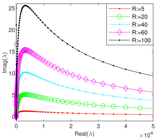
Let’s consider now the eigenproblem (1)–(2) equipped with the pure imaginary potential

$$q\left(x\right):=ı\alpha RV\left(x\right),$$

(5)

where $\alpha$ and R are real constants (wave number and Reynolds number, respectively) and $V\in L^{\infty }[0,\infty ).$

We have solved the eigenproblem (1)–(2) by mapped ChC when

$$\alpha :=1,\mathrm{and}V\left(x\right):=sin\left(x\right)exp(-x).$$

(6)

The eigenvalues for various Reynolds numbers are displayed in Figure 1. Their scattering in the complex plane is very similar to that which is only suggested in Figure 1 from [14]. However, a much larger number of eigenvalues is calculated and, more importantly, they all fully meet the conditions (3) and (4).

Figure 1. The eigenvalues of problem (1)–(2) when $V\left(x\right)$ is defined by (6) computed by mapped ChC with $N:=156$ and the scaling factor c takes on the value $1.75.$

The drift of eigenvalues with respect to order of approximation N is depicted in Figure 2a and the drift with respect to the scaling factor is reported in panel b of the same figure. Both show that no more than approximately 10 eigenvalues can be computed with an accuracy better than ${10}^{-5}$.

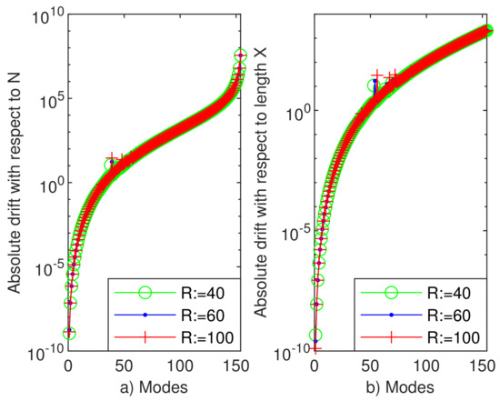
Figure 2. (a) The drift with respect to the order of approximation N for the first 156 eigenvalues. We have used values $N_1=156$ and $N_2=256$ when $c:=1.75;$ (b) the drift with respect to the scaling parameter c for the first 156 eigenvalues. We have worked with $c_1:=1.75$ and $c_2:=3.75$ when $N:=256.$

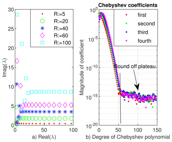
The result in solving the same problem with Chebfun is displayed in Figure 3. In panel (a), we observe a sort of numerical instability in computing the eigenvalues. Panel (b) of the same figure shows a smooth and deep decrease of Chebyshev coefficients of the first four eigenvectors down to ${10}^{-15}$ when N approximate 50. Then, a round off plateau follows. This signifies a correct behavior of Chebfun system.

Figure 3. (a) The leftmost ten eigenvalues of problem (1)–(2) when $V\left(x\right)$ is defined by (6) computed by Chebfun when the length of the integration interval is $X=5.75$; (b) the coefficients of the first four eigenvectors when $R:=100$.

3. Schrödinger Type Equations with Unbounded Potential at One Endpoint

3.1. Singular Inverse Square Potential

Let’s consider now Equation (1) to which we attach some separated boundary conditions in a and b and the potential q has the form

$$q\left(x\right):=f\left(x\right)+\frac{g\left(x\right)}{{\left(1+x\right)}^{\gamma }},$$

(7)

where f and g are analytic functions inside and on a Bernstein ellipse containing the canonical segment $[-1,1]$, and $\gamma \ge 0$. Problems of this type have applications in engineering and some of them have been solved in [15] by a spectral matrix method.

The weakly regular case

$$f\left(x\right):=2x^2,g\left(x\right):=5/\left(\left(1+x^2\right)+1\right)\mathrm{with}\mathrm{boundary}\mathrm{conditions},u^{\prime }\left(-1\right)=0=u\left(1\right),$$

(8)

where $\gamma \in \left(0,1\right)$ has been analyzed in [15].

In Table 1, we compare our results with those reported in [15] (Table 3) and in turn compared with the results obtained by other methods. Unfortunately, the differences are visible. In order to ensure the accuracy of the results obtained by ChC, we report the relative drift with respect to the order of approximation in Figure 4. For the fifteenth eigenvalue, it guarantees an accuracy of the order of ${10}^{-12}$. The variation of the magnitude of this eigenvalue in relation to $\gamma$ is the same, i.e., its magnitude increases with the value of this parameter. We mention that, for the last two values of $\gamma$, the point $x=-1$ is a singular one of nonoscillatory limit-circle type.

Table 1. The fifteenth eigenvalue to problem (1)–(8) computed by ChC for various exponents $\gamma$ and compared with those provided by a spectral matrix method.

$\mathit{\gamma }$	${\mathit{\lambda }}_{15}$ Computed by ChC	${\mathit{\lambda }}_{15}$ According to [15]
$0.40$	$5.220211963594209e+02$	$5.239182763990e+02$
$0.65$	$5.225998931867747e+02$	$5.281830147149e+02$
$0.90$	$5.237063568130833e+02$	$5.522447514722e+02$
$1.40$	$5.300573873839758e+02$	$\mathrm{not}\mathrm{computed}$
$1.90$	$5.482389946825781e+02$	$\mathrm{not}\mathrm{computed}$

Figure 4. The relative drift with respect to N of the first 250 eigenvalues of eigenproblem (1)–(8) computed by ChC; $N_1:=512$ and $N_2:=1024$-red dotted line and $N_1:=512$ and $N_2:=256$-green dotted line.

The first four eigenvectors of problem (1)–(8) are depicted in Figure 5. It is very clear that they satisfy boundary conditions (8). Their computation is a surplus compared to the work [15] where they are not calculated.

Figure 5. The first four eigenvectors of eigenproblem (1)–(8) computed by ChC when $N:=512$ and $\gamma :=0.65$.

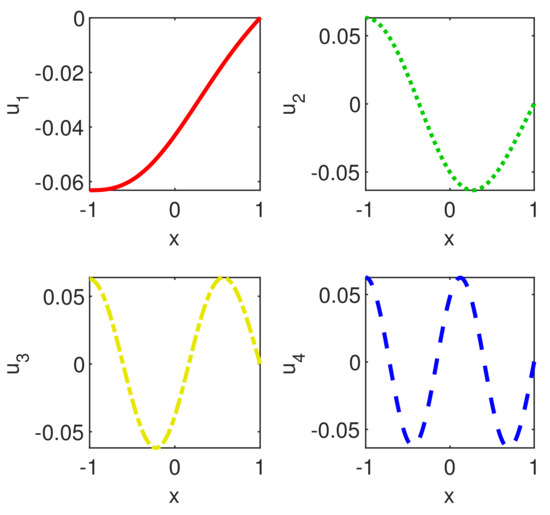
Their coefficients decrease smoothly and rapidly to the machine precision as it is apparent from Figure 6 panels (a) and (b).

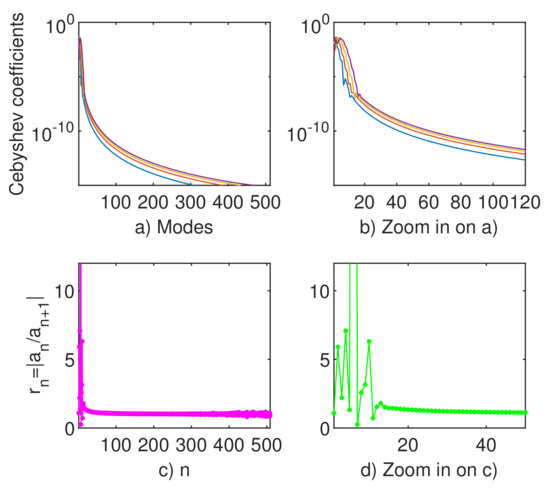
Figure 6. (a) The Chebyshev coefficients, obtained by FCT, for the first four eigenvectors of eigenproblem (1)–(8) computed by ChC when $N:=512$; (b) zoom in on the previous picture; (c) the ratio $r_n=\left|a_n/a_{n+1}\right|$ for the coefficients of the first eigenvector to the same problem; (d) zoom in on the previous picture. To the parameter $\gamma$ has assigned the numerical value $0.40.$

It is extremely important to point out that Figure 6c,d fully confirm the assertion in John Boyd’s work [16]. In this paper, it is stated that: the “most useful measure of the rate of convergence of a Chebyshev series is $r_n:=\left|a_n/a_{n+1}\right|$”. Moreover, he states that “$r_n$ must decrease to one as $n\to \infty$, if the function is singular at one or both end points ”.

We mention at the end of this section that ChC together with a removing technique of independent boundary conditions solved without problems all the singular eigenvalues problems from [15].

3.2. The Eigenproblem of Dunford and Schwartz

The generalized hypergeometric equation reads

$$-u^{″}+\frac{-242cosh\left(x\right)+241}{4{sinh}^2\left(x\right)}u=\lambda u,0<x<\infty .$$

(9)

In [17] Example 23, the author attaches to this equation the boundary conditions

$$\underset{x\to 0}{lim}\left[u\left(x\right)-2x{u}^{\prime }\left(x\right)\right]=0,u\left(\infty \right)=0,$$

(10)

the first one being of Friedrichs type. We must mention that so far we have not found a suitable technique to introduce this type of boundary conditions when working with ChC. This is why ChC has not even tried for this problem.

Anyway, in the proposed benchmark set of singular problems listed in [17], the problem (9)–(10) is considered one of the hardest.

The singularity in origin $\left({sinh}^2\left(x\right)=0\left(x^2\right)\mathrm{as}x\to 0\right)$ is of non-oscillatory limit-circle type with boundary functions $v\left(x\right):=\sqrt{x}$ and $w\left(x\right):=\sqrt{x}lnx.$ Thus, the boundary condition in origin comes from the equality $[u,v]=0$ where the symbol $\left[,\right]$ stands for the Wronskian of the functions u and v. The end point $b:=\infty$ is of type limit point non-oscillatory, so we attach the homogeneous Dirichlet boundary condition. Actually, in order to resolve the singularity at ∞, we solve this problem on the truncated interval

$$\left[\epsilon ,X\right],0<\epsilon \ll 1\mathrm{and}\mathrm{finite}X.$$

(11)

The best results (the most stable eigenvalues and the smoothest eigenvectors) have been obtained for $\epsilon :=1.e-06$ and $X:=12$. In order to improve the convergence of Chebfun, we use the option ‘splitting’,‘on’.

The first ten eigenvalues obtained are reported in Table 2. The first five of them reasonably approximate the exact eigenvalues ${\lambda }_n=-{\left(5-n\right)}^2$, $n=0,1,2,3,4$. The next five (the second column in Table 2) suggest the continuous spectrum on $\left(0,\infty \right)$ in the sense that the eigenvalues are becoming more and more crowded as their index increases. As a precaution not to consume space in excess, we limited ourselves to report only a few eigenvalues from our numerical experiments.

Table 2. The first ten eigenvalues of the Dunford and Schwartz eigenproblem (9)–(10).

$\mathit{j}$	Discrete ${\mathit{\lambda }}_{\mathit{j}}$ by Chebfun	$\mathit{j}$	“Continuous Spectrum by Chebfun
$0$	$-2.500000022514205e+01$	$5$	$1.578606493636769e-02$
$1$	$-1.599999998730550e+01$	$6$	$2.297844931237520e-01$
$2$	$-9.000000083479620e+00$	$7$	$6.369715876528872e-01$
$3$	$-4.000000202368167e+00$	$8$	$1.133491876230128e+00$
$4$	$-9.999995017483769e-01$	$9$	$1.761853804586405e+00$

The drift with respect to the length X (of the truncated integration interval from (11)) of the discrete eigenvalues of (9)–(10) is depicted in Figure 7. It clearly shows an accuracy of order at least ${10}^{-7}$ in computation of the first four eigenvalues.

Figure 7. The drift with respect to the length of the integration interval of the first five eigenvalues for the Dunford and Schwartz eigenproblem (9)–(10). We have used $X_1:=12$, $X_2:=8$-red circled line and $X_1:=10$, $X_2:=8$-green starred line with $\epsilon :=1.e-06$ in (11).

The first four eigenvectors of Dunford and Schwartz eigenproblem are displayed in Figure 8. They look plausible viz. the number of their roots.

Figure 8. A zoom in the first four eigenvectors of Dunford Schwartz eigenproblem (9)–(10) computed by Chebfun with $\epsilon :=1.e-06$ and $X:=12$ in (11).

With its two singularities, this problem has proved to be one of the most difficult and expensive in terms of computing elapsed time. However, Chebfun has provided remarkable numerical results.

3.3. A Nasty Eigenproblem with Logarithmic Potential

We will consider in this subsection the eigenproblem (1) supplied with homogeneous Dirichlet boundary conditions and the potential defined by

$$q\left(x\right):=ln\left(x\right).$$

(12)

The problem is solved in [17] by the SLTSTPAK package on the interval $\left[0,4\right]$, as Example 11, and is considered as a regular problem that looks singular.

3.3.1. ChC Method

The problem contains that nasty $q\left(x\right)$, but the classical ChC works extremely fast and accurate. The following simple MATLAB code produces the eigenpairs of the matrix A:

    N=512;                % The approximation order

    [x,D]=chebdif(N,2);        % Differentiation matrices [Weideman & Reddy]

    k=2:N;                % Kept modes

    xbc=x(k); Deig=D(k,k,2);        % Kept nodes and matrix

    A=-Deig/4+diag(log((xbc+1)*2));    % [0,4] shifted to [-1,1]

    [U,S]=eig(A); [t,o]=sort(diag(S)); S=S(o); U=U(:,o);

    disp(S(1:24))              % Compute,sort and display

We enforce the boundary condition by the removing technique of independent boundary conditions introduced in [18]. Thus, we delete the first and the last rows and columns in the second order Chebyshev differentiation matrix $D(:,:,2)$ and obtain the matrix $Deig$. The nodes $x_1$ and $x_N$ of the Chebyshev–Gauss–Lobatto system are eliminated as slaves and after the problem is solved they are given-back. Actually, we simply add two zeros, one in the first and another in the last position of each eigenvector.

3.3.2. Chebfun Method

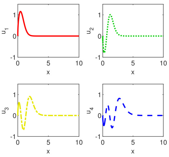
In order to avoid the singularity of $q\left(x\right)$ in origin, we solve the same problem by Chebfun on the modified (truncated) domain of the form (11), namely $\left[1.e-08,4\right]$. The first four eigenvectors are displayed in Figure 9. They look fairly smooth and they do not seem affected at all by the singularity. However, our numerical experiments showed that their coefficients do not decrease smoothly, and this is due to the singularity of $q\left(x\right)$.

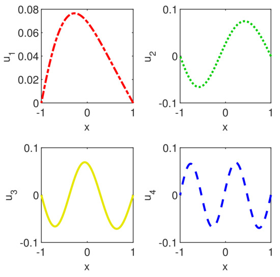
Figure 9. First four eigenvectors of nasty $q\left(x\right)$ eigenproblem defined by (12) computed by Chebfun.

Anyway, no warning has been displayed by Chebfun when the option ’splitting’,’on’ has been invoked.

3.3.3. ChC vs. Chebfun

The first and the twenty-fourth eigenvalues of this eigenproblem computed by ChC, Chebfun, and reported in [17] are displayed in Table 3. If, with respect to the first eigenvalue, we observe that they coincide up to the fifth decimal, this does not happen for the value of the twenty-fourth eigenvalue. Thus, in order to separate the “good” eigenvalues from the “bad” ones, i.e., numerically inaccurate eigenvalues, we use again the concept of relative drift, now with respect to the order of approximation N. Actually, the relative drift of eigenvalues computed by ChC and reported in Figure 10 shows a coincidence of at least order ${10}^{-11}$ for the first twenty-fourth eigenvalue computed by ChC. In other words, it means that the relative drift is resolution independent with respect to N for the outcomes of ChC method, and the method is numerically stable. Inspecting now the Table 3, we can conclude that the eigenvalues computed by ChC and Chebfun are more accurate than those reported in [17], especially for large values of N.

Table 3. The first and the twenty-fourth eigenvalues of nasty eigenproblem (12) computed by three different methods.

$\mathit{j}$	${\mathit{\lambda }}_{\mathit{j}}$ Computed by ChC	${\mathit{\lambda }}_{\mathit{j}}$ Computed by Chebfun	${\mathit{\lambda }}_{\mathit{j}}$ According to [17]
$0$	$1.124816809695236e+00$	$1.124816818756614e+00$	$1.1248168097$
$23$	$3.557030079371902e+02$	$3.557030097207584e+02$	$385.92821596$

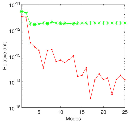
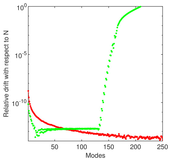
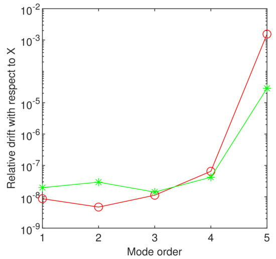
Figure 10. The relative drift with respect to the order of approximation of the first twenty-four eigenvalues of eigenproblem (12). We have used $N_1:=512$ and $N_2:=256$ to get the red dotted line and $N_1:=128$ and $N_2:=256$ to get the green starred line.

The eigenvectors computed by the two methods look practically identical, so we present in Figure 9 only those obtained through Chebfun. Now, it is clear that the price paid by Chebfun to provide eigenvalues with the same order of accuracy as ChC is the truncation of the domain.

3.4. Quantum-Mechanical Potential with Weierstrass Spectrum

We are concerned now in Equation (1) equipped with the Weierstrass–Mandelbrot potential

$$q\left(x\right):=\left({\omega }^2-(1/4)\right)/x^2,\omega >0,$$

(13)

along with boundary conditions

$$u\left(0\right)=u(\infty )=0.$$

(14)

In order to avoid singularity in origin, in [5], it is suggested to use the modified potential

$$q\left(x\right):=\left({\omega }^2-(1/4)\right)/{\left(x+\epsilon \right)}^2,\omega >0\mathrm{and}\epsilon \to 0.$$

(15)

We have solved the problem (1)–(15) by Chebfun with truncation when $\epsilon :=1e-06$.

For various values of $\omega$, the outcomes are displayed in Table 4.

Table 4. The dependence of eigenvalues to problem (1)–(15) on the parameter $\omega$. Chebfun used $X:=6.5.$

Eigenvalues	${\mathit{\omega }}^2=3$	${\mathit{\omega }}^2=1$	${\mathit{\omega }}^2=0.1$
${\lambda }_1$	$-1.897744652003916e+06$	$-1.424952616037219e+04$	$-3.196897435172694e+03$
${\lambda }_2$	$-5.044194522302225e+04$	$-2.661017492401879e+01$	$1.968974336050451e-01$
${\lambda }_3$	$-1.340869422704913e+03$	$4.642654594499618e-02$	$1.063397994963452e+00$
${\lambda }_4$	$-3.563883241196163e+01$	$1.019400854595006e+00$	$2.604158839443699e+00$
${\lambda }_5$	$-9.456852914299816e-01$	$2.743653826764785e+00$	$4.812930809683166e+00$
${\lambda }_6$	$4.537872010841966e-01$	$5.200157281942666e+00$	$7.687329560169019e+00$

We think some comments are important at this time. The increase of the number of negative eigenvalues with the increase of parameter $\omega$ is in qualitative agreement with the conclusions from the paper [5] Section 5. Unfortunately, we have not been able to prove that the calculated spectrum is indeed a Weierstrass one. This remains an open issue. This problem is listed in the paper [17] but is not actually solved so we do not have a term of comparison. However, our numerical experiments showed that Chebfun is stable with respect to the length X in the range $\left[5,12\right].$

4. Schrödinger Type Equations with an Interior Singularity

Here, we analyze first the so called Boyd’s eigenproblem. It is called singular if $q\in L\left[\alpha ,\beta \right]$ for any $\left[\alpha ,\beta \right]\subset \left[a,b\right]$ and $q\notin L\left[a,b\right].$ For two real numbers a and b, such that $-\infty <a<0<b<\infty ,$ the potential $q\left(x\right)$ is defined by

$$q\left(x\right):=-1/x.$$

(16)

We attach the homogeneous Dirichlet boundary conditions

$$u\left(a\right)=u\left(b\right)=0,$$

(17)

to Equation (1) with q defined in (16).

In [19], the author characterizes this problem as “an unusually nasty eigenproblem because the eigenmodes are logarithmically singular on the interior of the interval.” 

On the other hand, from the mathematical point of view, in [20], the authors show that the eigenproblem (1), (16) and (17) has a unique solution which has a discrete real spectrum $\left\{{\lambda }_n,n\in {\mathbb{N}}_0\right\}$ where

$$-\infty <{\lambda }_0\le {\lambda }_1\le {\lambda }_2\le \dots \le {\lambda }_n\le {\lambda }_{n+1}\le ...,\mathrm{and}\underset{n\to \infty }{lim}{\lambda }_n=\infty .$$

The corresponding real-valued eigenfunctions $\left\{u_n,n\in {\mathbb{N}}_0\right\}$ satisfy the Equation (1) and the Dirichlet boundary conditions (17) and the following properties for $n\in {\mathbb{N}}_0$:

• $u_n:\left[a,b\right]\to \mathbb{R}$ and $u_n\in C\left[a,b\right];$
• $u_n\in C^2[a,0)\cup C^2(0,b];$
• $u_n\left(0\right)=0;$
• in general $u_n^{\prime }\left(0^{-}\right)\ne$$u_n^{\prime }\left(0^{+}\right)$, but both limits are finite;
• ${\int }_a^b{u}_n\left(x\right)u_m\left(x\right)dx={\delta }_{n,m},$ for $n\ne m\in {\mathbb{N}}_0;$
• $\left\{u_n,n\in {\mathbb{N}}_0\right\}$ is a complete orthonormal set in the Hilbert space $L^2\left[a,b\right];$
• degeneracy may occur, but no eigenvalue can have multiplicity greater than two.

4.1. Chebfun Results

The Chebfun code has failed to solve this problem in form (1), (16) and (17). However, in order to solve it numerically, we use a regularized version of $q\left(x\right)$, namely

$$q\left(x,\epsilon \right):=-\frac{x}{x^2+{\epsilon }^2},0<\epsilon \ll 1,$$

(18)

in the sense of distributions, i.e., ${lim}_{\epsilon \to 0}q\left(x,\epsilon \right)=-\delta \left(\frac{1}{x}\right),$ where, as usual, $\delta$ stands for Dirac distribution. With this approximation of the original coefficient $q\left(x\right)$, the eigenproblem becomes a regular one. It is temping to hope that the perturbed set of eigenvalues $\left\{{\lambda }_n\left(\epsilon \right),n\in {\mathbb{N}}_0\right\}$ and of eigenvectors $\left\{u_n\left(x,\epsilon \right),n\in {\mathbb{N}}_0\right\}$ approaches in some sense the corresponding sets of the original problem when $\epsilon \to 0.$

Actually, with Chebfun computations, we have used $\epsilon :=1.e-05$ in (18) on the integration interval $\left[-10,10\right]$. The length of this interval is arbitrary, so, in order to back the results obtained by Chebfun, we use an alternative method in Section 4.2.

4.2. Sinc Collocation Results

With the SiC, we have used the order of approximation N in the range 200–500 and the scaling factor $h:=0.1$. To the parameter, $\epsilon$ in (18) has been assigned the same value, namely $1e-05$.

The first four vectors obtained are displayed in Figure 11. They are continuous in origin but with discontinuous derivatives. They are also mutually orthogonal as it clearly results from the left panel (a) Figure 12.

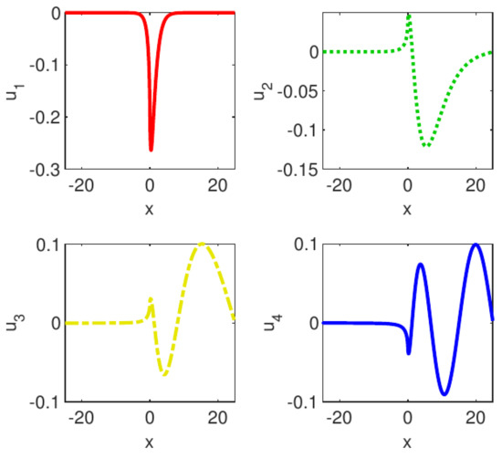
Figure 11. The first four eigenvectors of Boyd’s eigenproblem computed by SiC when $N:=500$ and $h:=0.1$. The logarithmic singularity is clearly visible in origin.

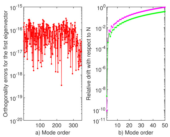
Figure 12. (a) The departure from orthogonality of the first eigenvector with respect to the subsequent 499 of it when SiC solves problem (1), (16) and (17); (b) the relative drift with respect to order of approximation N of the first 50 eigenvalues computed by SiC. The magenta dotted line has been obtained with $N_1:=350$ and $N_2:=250$, and the green dotted line has been obtained $N_1:=200$ and $N_2:=250.$ In both cases, $\epsilon :=1.e-06.$

Thus, the first five items enumerated above are plainly verified. Moreover the spectrum is real, discrete, and converges to ∞ as $N\to \infty .$

In Table 5, we report the first six eigenvalues computed by SiC, Chebfun, and by the SLEIGN package according to [20]. In the latter case, the authors worked with $\epsilon :=1.e-03$ on the interval $\left[-10,10\right]$. However, in the right panel b) of Figure 12, the relative drift of the first eigenvalue is around $O\left({10}^{-10}\right)$, which means an error of the same order. Unfortunately, the accuracy decreases rather rapidly and thus we can trust only the first five, six eigenvalues.

Table 5. The first six eigenvalues to Boyd’s eigenproblem computed by three different methods.

$\mathit{j}$	${\mathit{\lambda }}_{\mathit{j}}$ Computed by SiC	${\mathit{\lambda }}_{\mathit{j}}$ Computed by Chebfun	${\mathit{\lambda }}_{\mathit{j}}$ According to [20]
$0$	$-9.606831952007443e-01$	$-9.794200447802075e-01$	$-0.9841$
$1$	$-7.671890334071728e-02$	$-7.751928355451891e-02$	$-0.0778$
$2$	$2.722504457479860e-01$	$2.732439098153830e-01$	$0.2727$
$3$	$3.076092365139790e-01$	$3.092576560488862e-01$	$0.3092$
$4$	$6.713233935551861e-01$	$6.754139419849143e-01$	$0.6754$
$5$	$8.358600253567475e-01$	$8.403112262426201e-01$	$0.8396$

In order to justify the convergence of the eigenvalues calculated with SiC when $\epsilon$ tends to zero, we have estimated the drift of the first 100 eigenvalues with respect to this parameter. This is reported in Figure 13, and it gives us confidence that this convergence does take place. What is interesting and still unexplained is the fact that the largest oscillations appear in the calculation of the first eigenvalues after which the algorithm stabilizes.

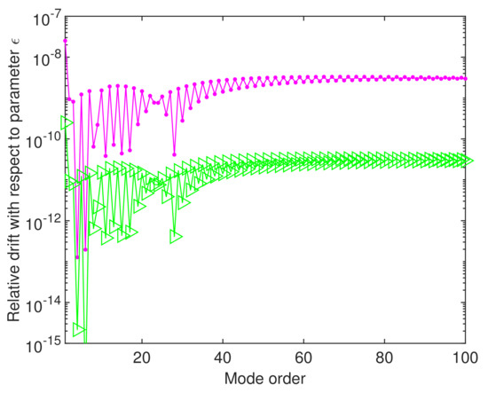
Figure 13. The relative drift with respect to the parameter $\epsilon$ of the first 100 eigenvalues computed by SiC with $N:=350$ and $h:=0.1$. The magenta dotted line has been obtained with ${\epsilon }_1:=1e-04$ and ${\epsilon }_2:=1e-06$, and the green arrowhead line has been obtained j and ${\epsilon }_2:=1e-06.$

4.3. Zero-Pairs of Bessel Functions

In [21], the author considers a very interesting generalization to the Bessel’s problem. He tries to answer the question of finding zero-pairs of Bessel functions of order $\nu$, i.e., some numbers a and b for which there exists a Bessel function of order $\nu$ which vanishes simultaneously at a and b. We will consider this question from a numerical point of view in searching a deeper understanding of the singularity in origin of Bessel’s eigenproblem.

This new problem reads

$$\left\{\begin{array}{c}{u}^{″}+\left[\lambda +\frac{\left(\frac{1}{4}-{\nu }^2\right)}{{\left(x-\tau \right)}^2}\right]u=0,-1<x<1,\nu ,\tau \in \mathbb{R},\\ u\left(\pm 1\right)=0.\end{array}\right.$$

(19)

For given $\tau >1$ (or $\tau <-1$), we have a regular Sturm–Liouville problem with eigenvalues

$$0<{\lambda }_1\left(\tau \right)<{\lambda }_2\left(\tau \right)<\dots .$$

Chebfun confirms this statement and solves this regular problem in no time. It is easy to show that the functions ${\lambda }_n\left(\tau \right)$ are analytic for the above values of $\tau .$ The author of [21] asks for properties of the analytic continuation of ${\lambda }_n\left(\tau \right)$ into the complex plane. For $\nu \in \left[1/3,1/2\right]$ in the same paper [21], it is shown that ${\lambda }_n\left(\tau \right)$, $n\in \mathbb{N}$ are analytic in the domain $\mathbb{C}\setminus \left[-1,1\right]$ and at $\tau :=\infty$, and these functions are also analytic on the segments $\tau \pm i0$ for $-1<\tau <1.$ They can be extended continuously into $\tau =\pm 1$, respectively.

With the following simple Chebfun code,

x=chebfun(‘x’,[-1, 1],‘splitting’,‘on’); nu=1/3;tau=0; %tau=1;

L=chebop(-1,1);

L.op =@(x,y)-((x-tau)^2)*diff(y,2)+((nu^2)-1/4)*y;

L.rbc=0;  L.lbc=0;

M=chebop(-1,1); M.op=@(x,y) ((x-tau)^2)*y; M.bc=[ ];

% Find the first 40 eigenvalues of the eigenpencil (L, M)

[V,D]=eigs(L,M,40); sort(diag(D))

we have computed some eigenpairs of problem (19) for various $\tau$ and $\nu$. They are reported in the first two columns of Table 6.

Table 6. The first eight eigenvalues of eigenproblem (19) computed by Chebfun for $\tau :=0$ and $\tau :=1/4$ (first two columns). In the third column, we report the eigenvalues of the same problem computed by ChC when $\tau :=0$. In both methods, we have assumed $\nu =1/3$.

$\mathit{j}$	${\mathit{\lambda }}_{\mathit{j}}$$\mathit{\tau }:=0,$$\mathit{\nu }=1/3$ Chebfun	${\mathit{\lambda }}_{\mathit{j}}$$\mathit{\tau }:=1/4,$$\mathit{\nu }=1/3$ Chebfun	${\mathit{\lambda }}_{\mathit{j}}$$\mathit{\tau }:=0,$$\mathit{\nu }=1/3$ ChC
$0$	$8.427067009456547e+00$	$5.400563866142070e+00$	$8.427945713285165e+00$
$1$	$8.571978456544725e+00$	$1.503383426547553e+01$	$8.661777916480734e+00$
$2$	$3.640104840502095e+01$	$2.332141941007685e+01$	$3.640525136075537e+01$
$3$	$3.689758359379723e+01$	$5.388134332882591e+01$	$3.720851434888583e+01$
$4$	$8.411229915649267e+01$	$6.489190302110852e+01$	$8.412057813169606e+01$
$5$	$8.511762862999629e+01$	$9.708229958053987e+01$	$8.575213457278441e+01$
$6$	$1.515639240123626e+02$	$1.498879163534515e+02$	$1.515775098405456e+02$
$7$	$1.532164600154869e+02$	$1.529282181428597e+02$	$1.542668794303226e+02$

It is very important to note that, in solving this eigenproblem both methods, ChC as well as Chebfun, have encountered some difficulties. Thus, for the values of $\tau$ close to zero Chebfun displays the following warning: Maximum dimension reached. Solution may not have converged. This warning prompted us to look for a way to validate these results. Consequently, we have solved the problem with the classic ChC. For an unusually large approximation order $N:=2028$, i.e., half of that used by Chebfun, ChC produced the third column of Table 6.

The drift of the first ten eigenvalues is depicted in Figure 14. This figure suggests a sort of lack of numerical stability and also that we can not hope for a better accuracy than ${10}^{-3}$ in approximating these pairs of quasi double eigenvalues.

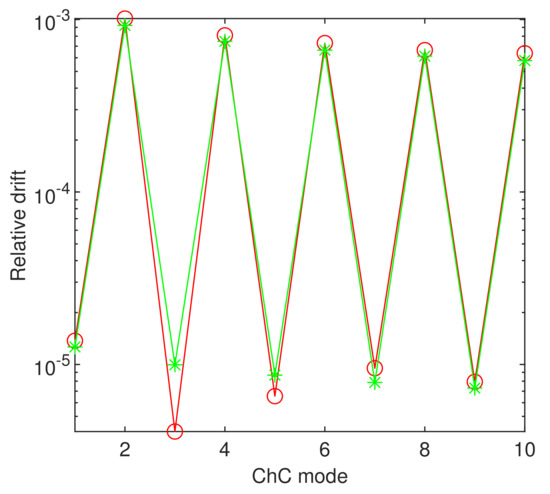
Figure 14. The relative drift with respect to N of the first ten eigenvalues of eigenproblem (19) when $\nu :=1/3$ and $\tau :=0$. The red circled line corresponds to $N_1:=1900$ and $N_2:=2000$, and the green starred line corresponds to $N_1:=2100$ and $N_2:=2000.$

The first four eigenvectors of problem (19) computed by Chebfun when $\tau :=0$ and $\nu :=1/3$ are displayed in Figure 15. From this figure, it is clear that, in pairs, i.e., for indices 1 and 2, 3, and 4, etc. The vectors are identical over the range $\left[-1,0\right].$ Moreover, and at the same time more interesting, they become perfectly symmetric with respect to the horizontal axis on the interval $\left[0,1\right]$. Actually, we have found symmetric zero-pairs for Bessel function of order $1/3.$

Figure 15. The first four eigenvectors of problem (19) computed by Chebfun when $\tau :=0$ and $\nu :=1/3$.

The dependence of the first two sets of eigenvalues ${\lambda }_0$ and ${\lambda }_1$ of problem (19) on $\tau$ is depicted in Figure 16. The lower curve corresponds to ${\lambda }_0\left(\tau \right)$, $\tau \in \left[0,1\right].$ This figure has to be seen with a symmetric part on $\left[-1,0\right]$. In order to smooth these curves we have used the MATLAB pchip code that performs a piecewise Hermite cubic interpolation.

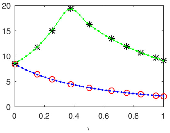
Figure 16. The dependence of the first two sets of eigenvalues ${\lambda }_0$ (lower circled curve) and ${\lambda }_1$ of problem (19) on $\tau$ when $\nu :=1/3$.

In our opinion, this last figure suggests that, in origin, the so-called phenomenon of level crossing of eigenvalues occurs as described in [22] (p. 350) (see also [23]). Due to the scale at which the curves are drawn, the first two eigenvalues ${\lambda }_0$ and ${\lambda }_1$, from the first column of the Table 6, appear to be superimposed, but actually they are only very nearly, i.e., almost double.

Along with the results displayed in Table 6, we can answer the question formulated in the title of paper [24]. Thusfar, close to the origin multiple eigenvalues are not rare at all for the Bessel problem (19). Moreover, this result is in the spirit of Theorem 6.6 from [24] on degeneracies in the spectra of self-adjoint operators of Schrödinger type.

Other several numerical results are in progress with respect to this challenging problem.

5. Extension to a Regular 2D Schrödinger Equation

In order to fix ideas, let’s consider a 2D Schrödinger eigenproblem. It reads

$$-\Delta u+q(x,y)u=\lambda u,-1<x,y<1,$$

(20)

along with homogeneous Dirichlet boundary conditions on the sides of the standard square $\left[-1,1\right]\times \left[-1,1\right],$

$$u\left(\pm 1,y\right)=u\left(x,\pm 1\right)=0.$$

(21)

With respect to the problem (20)–(21), also called the generalized Helmholtz problem, Rayleigh, on physical grounds, and then Hilbert, Weyl, and others proved the so-called Ohm–Rayleigh principle. It states that, on any bounded domain $\Omega$ with compact closure, the problem (20)–(21) has a basis of eigenfunctions, and any two eigenfunctions having distinct eigenvalues are orthogonal (see [25]). Moreover, the Laplace operator is separable and in operator notation we can write

$$\Delta =\mathit{A}\otimes \mathit{I}+\mathit{I}\otimes \mathit{B},\mathit{I}\mathrm{the}\mathrm{identity},$$

where $\mathbf{A}:={\partial }^2/\partial x^2$, $\mathbf{B}:={\partial }^2/\partial y^2$ and ⊗ stands for the direct or tensor product.

We have solved this problem by ChC. The second order partial derivatives have been computed using the MATLAB function kron as it is suggested in [7]. The main disadvantage of this approach for solving 2D problems is that the order of the involved matrices are large, i.e., it equals $N^2\times N^2$ (the so-called the curse of dimensionality).

For $q\left(x,y\right):=\left(1+x^2\right)\left(1+y^2\right)$, the eigenproblem (20)–(21) have been solved in [26] by CP methods which are piecewise perturbation methods.

Fortunately, our results plainly confirm these outcomes as it is clear from Table 7. Actually, in order to carry out this comparison, we have worked in the shifted domain $\left[-5.5,5,5\right]\times \left[-5.5,5.5\right].$ We notice that the discretization involved in [26] leads to matrices of the same large order $N^2\times N^2.$

Table 7. Some eigenvalues of eigenproblem (20)–(21) computed by ChC with $N=52$ and CP.

j	${\mathit{\lambda }}_{\mathit{j}}$ Computed by ChC	${\mathit{\lambda }}_{\mathit{j}}$ According to [26]
1	$3.195918085202131$	$3.1959181$
$2_a$	$5.526743874391412$	$5.5267439$
$2_b$	$5.526743874395398$	$5.5267439$
3	$7.557803326788490$	$7.5578033$
4	$8.031272340314583$	$8.0312723$
5	$8.444581361568989$	$8.4445814$
$6_a$	$9.928061056960347$	$9.9280611$
$6_b$	$9.928061056962180$	$9.9280611$
$7_a$	$1.131181705061307e+01$	$11.3118171$
$7_b$	$1.131181705061503e+01$	$11.3118171$
8	$1.210325357879031e+01$	$12.1032536$
9	$1.220117896804022e+01$	$12.2011790$
10	$1.333233127109757e+01$	$13.3323313$

We observe that eigenvalues ${\lambda }_2$, ${\lambda }_6$ and ${\lambda }_7$ are double degenerate.

In order to assess the accuracy in computing the eigenenergies, we display in Figure 17 the drift with respect to N of the first 25 eigenvalues.Thus, we can hope for a precision better than ${10}^{-6}$ for all these eigenvalues.

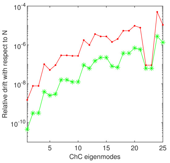
Figure 17. In a log-linear plot, we display the relative drift of the firs 25 eigenvalues computed by ChC. Thus, the red dotted line corresponds to $N_1:=36$ and $N_2:=40$, and the green starred line corresponds to $N_1:=52$ and $N_2:=40$.

Some eigenvectors are reported in Figure 18. In order to save space and to get clarity, we have used the option off for axis and have interpolated on a finer grid in order to plot.

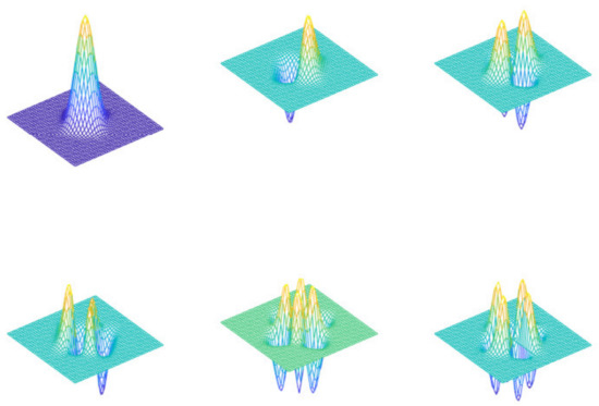
Figure 18. From upper left to right down, we display the first and the eigenvectors corresponding, respectively, to eigenvalues $2_a,$ 4, $6_a$, $7_a$, and 12.

In fact, we easily calculated the first one hundred eigenpairs using the MATLAB eig function.

6. Conclusions and Some Open Problems

In this paper, we have added a series of new singularities to the Schrödinger equation in order to test the qualities of spectral methods in resolving them. A first finding is that both ChC and Chebfun operate accurately in the case of complex potentials. However, as a general remark, we must underline once again the high qualities of both classes of methods used and note that ChC has been successfully extended to a 2D regular problem.

Many other singular SL eigenproblems are waiting to be analyzed, using spectral methods, in order to better understand their possibilities and limitations of application.

A particular open problem that first comes to mind, and for which there are some results in progress, is the simultaneous dependence of the eigenvalues of Bessel’s equation on both parameters $\tau$ and $\nu$. This could shed more light on the singularity in origin for various problems attached to this classical equation. a second would be a more detailed analysis of the Weierstrass spectrum.

References

- Gheorghiu, C.-I. Accurate Spectral Collocation Computation of High Order Eigenvalues for Singular Schrödinger Equations. Computation 2021, 9, 2. [Google Scholar] [CrossRef]
- Shizgal, B. Spectral Methods in Chemistry and Physics. Application to Kinetic Theory and Quantum Mechanics; Springer: Berlin/Heidelberg, Germany, 2015. [Google Scholar] [CrossRef]
- Zettl, A. Sturm–Liouville Theory; A. M. S. Providence: Providence, RI, USA, 2005. [Google Scholar]
- Frank, W.M.; Land, J.D.; Spector, R.M. Singular Potentials. Rev. Mod. Phys. 1971, 43, 36–98. [Google Scholar] [CrossRef]
- Berry, M.V.; Lewis, S.V. On the Weierstrass-Mandelbrot Fractal Function. Proc. R. Soc. Lond. A 1980. [Google Scholar] [CrossRef]
- Gheorghiu, C.-I. Spectral Methods for Non-Standard Eigenvalue Problems. Fluid and Structural Mechanics and Beyond; Springer: Berlin/Heidelberg, Germany, 2014. [Google Scholar]
- Weideman, J.A.C.; Reddy, S.C. A MATLAB Differentiation Matrix Suite. ACM Trans. Math. Softw. 2000, 26, 465–519. [Google Scholar] [CrossRef]
- Schonfelder, J.L. Chebyshev Expansions for the Error and Related Functions. Math. Comput. 1978, 32, 1232–1240. [Google Scholar] [CrossRef]
- Roy, A.K. The generalized pseudospectral approach to the bound states of the Hulthén and the Yukawa potentials. Pramana J. Phys. 2005, 65, 1–15. [Google Scholar] [CrossRef]
- Driscoll, T.A.; Bornemann, F.; Trefethen, L.N. The CHEBOP System for Automatic Solution of Differential Equations. BIT 2008, 48, 701–723. [Google Scholar] [CrossRef]
- Driscoll, T.A.; Hale, N.; Trefethen, L.N. Chebfun Guide; Pafnuty Publications: Oxford, UK, 2014. [Google Scholar]
- Trefethen, L.N.; Birkisson, A.; Driscoll, T.A. Exploring ODEs, SIAM: Philadelphia, PA, USA, 2018.
- Brown, B.M.; McCormack, D.K.R.; Evans, W.D.; Plum, M. On the spectrum of second-order differential operators with complex coefficients. Proc. R. Soc. A 1999, 455, 1235–1257. [Google Scholar] [CrossRef]
- Brown, B.M.; Langer, M.; Marletta, M.; Tretter, C.; Wagenhofer, M. Eigenvalue bounds for the singular Sturm–Liouville problem with a complex potential. J. Phys. A: Math. Gen. 2003, 36, 3773–3787. [Google Scholar] [CrossRef]
- Magherini, C. A corrected spectral method for Sturm–Liouville problems with unbounded potential at one endpoint. J. Comput. Appl. Math. 2020, 364. [Google Scholar] [CrossRef]
- Boyd, J.P. A Chebyshev polynomial method for computing analytic solutions to eigenvalue problems with application to the anharmonic oscillator. J. Math. Phys. 1978, 19, 1445–1456. [Google Scholar] [CrossRef]
- Pryce, J.D. A Test Package for Sturm–Liouville Solvers. ACM T. Math. Softw. 1999, 25, 21–57. [Google Scholar] [CrossRef]
- Hoepffner, J. Implementation of Boundary Conditions. Available online: http://www.lmm.jussieu.fr/hoepffner/boundarycondition.pdf (accessed on 25 August 2012).
- Boyd, J.P. Traps and Snares in Eigenvalue Calculations with Application to Pseudospectral Computations of Ocean Tides in a Basin Bounded by Meridians. J. Comput. Phys. 1996, 126, 11–20. [Google Scholar] [CrossRef]
- Everitt, W.N.; Gunson, J.; Zettl, A. Some comments on Sturm–Liouville eigenvalue problems with interior singularities. J. Appl. Math. Phys. ZAMP 1987, 38, 813–838. [Google Scholar] [CrossRef]
- Volkmer, H.W. Eigenvalue problems for Bessel’s equation and zero-pairs of Bessel functions. Stud. Sci. Math. Hung. 1999, 35, 261–280. [Google Scholar]
- Bender, C.; Orszag, S. Advanced Mathematical Methods for Scientists and Engineers; McGraw-Hill: New York, NY, USA, 1978. [Google Scholar]
- Trefethen, L.N. Analyticity at Eigenvalue Near-Crossings. Available online: https://www.chebfun.org/examples/linalg/CrossingsAnalyticity.html (accessed on 20 January 2020).
- Teytel, M. How Rare Are Multiple Eigenvalues? Comm. Pure Appl. Math. 1999, 52, 917–934. [Google Scholar] [CrossRef]
- Birkhoff, G.; Lynch, R.E. Numerical Solutions of Elliptic Problems; Society for Industrial and Applied Mathematics: University City, PA, USA, 2014; pp. 38–40. [Google Scholar] [CrossRef]
- Ixaru, L. New numerical method for the eigenvalue problem of the 2D Schrödinger equation. Comput. Phys. Commun. 2010, 181, 1738–1742. [Google Scholar] [CrossRef]
Publisher’s Note: MDPI stays neutral with regard to jurisdictional claims in published maps and institutional affiliations. |
© 2021 by the author. Licensee MDPI, Basel, Switzerland. This article is an open access article distributed under the terms and conditions of the Creative Commons Attribution (CC BY) license (https://creativecommons.org/licenses/by/4.0/).