
A Note on the Birnbaum–Saunders Conditionals Model


Abstract
1. Introduction
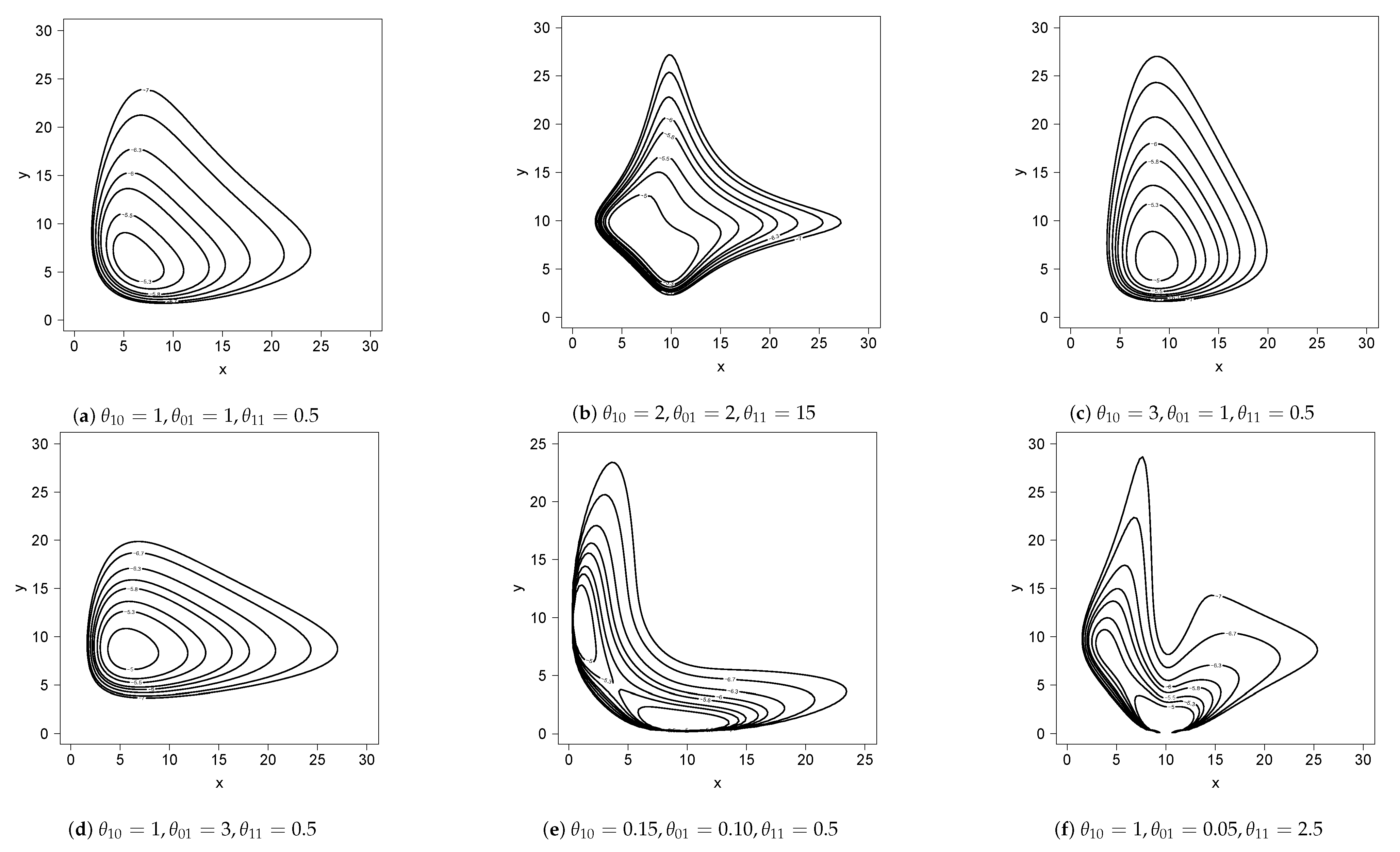
2. The Proposed Conditionally Specified Model
2.1. Drawing Values from the Model
| Algorithm 1 Metropolis–Hastings algorithm. |
|
3. Estimation
4. Simulation Study
5. Applications
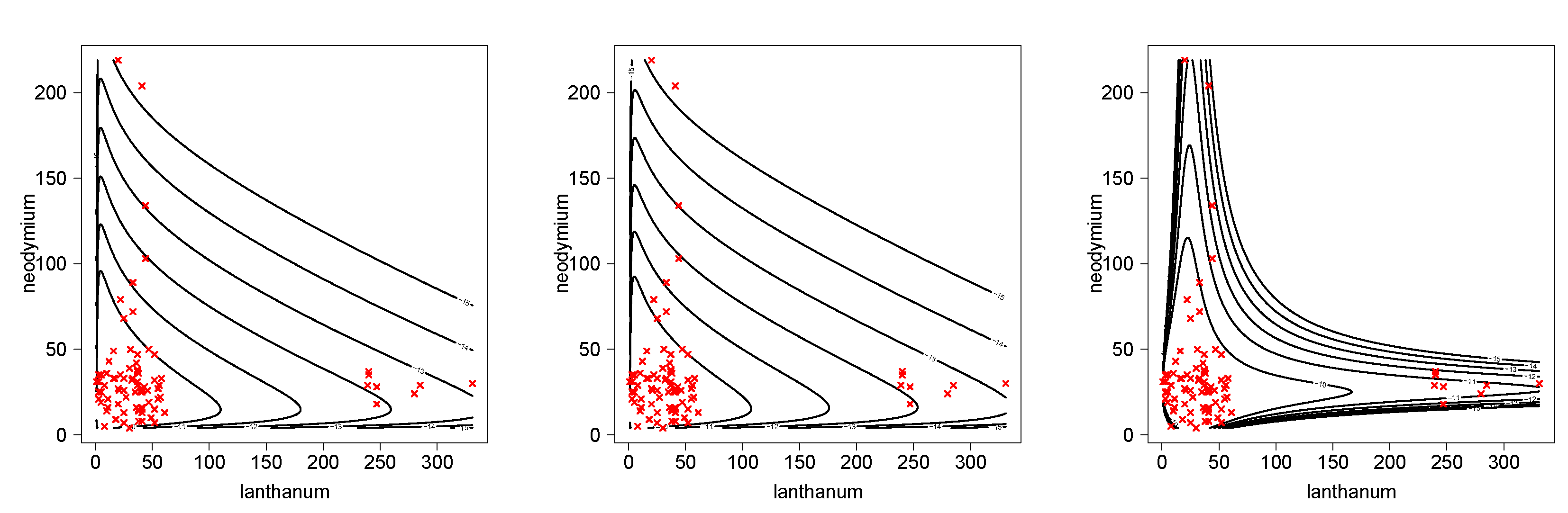
5.1. Minerals Data Set
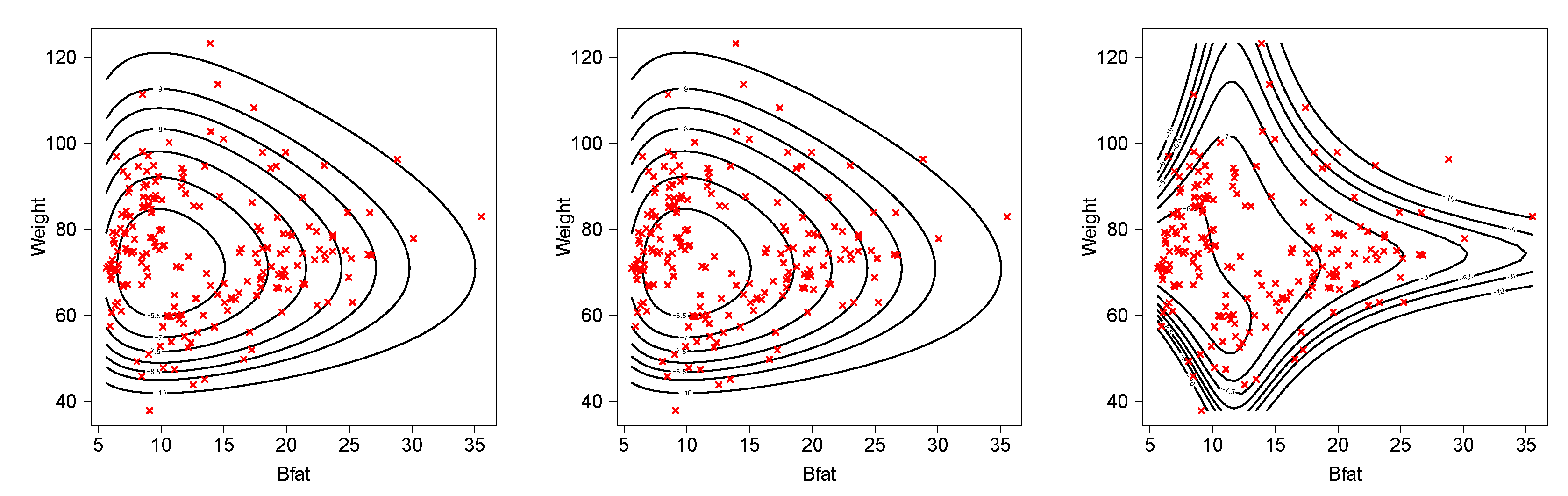
5.2. Australian Athletes Data Set
6. Discussion
Supplementary Materials
Author Contributions
Funding
Data Availability Statement
Acknowledgments
Conflicts of Interest
Appendix A
References
- Leiva, V. The Birnbaum-Saunders Distribution; Academic Press: New York, NY, USA, 2016. [Google Scholar]
- Balakrishnan, N.; Kundu, D. Birnbaum-Saunders distribution: A review of models, analysis, and applications. Appl. Stoch. Model. Bus. Ind. 2019, 35, 4–49. [Google Scholar] [CrossRef]
- Reyes, J.; Barranco-Chamorro, I.; Gallardo, D.I.; Gómez, H.W. Generalized Modified Slash Birnbaum-Saunders Distribution. Symmetry 2018, 10, 724. [Google Scholar] [CrossRef]
- Martínez-Flérez, G.; Barranco-Chamorro, I.; Bolfarine, H.; Gómez, H.W. Flexible Birnbaum–Saunders Distribution. Symmetry 2018, 11, 1305. [Google Scholar] [CrossRef]
- Gómez-Déniz, E.; Gómez, L. The Rayleigh Birnbaum Saunders Distribution: A General Fading Model. Symmetry 2020, 12, 389. [Google Scholar] [CrossRef]
- Mazucheli, J.; Leiva, V.; Alves, B.; Menezes, A.F.B. A New Quantile Regression for Modeling Bounded Data under a Unit Birnbaum–Saunders Distribution with Applications in Medicine and Politics. Symmetry 2021, 13, 682. [Google Scholar] [CrossRef]
- Arnold, B.C.; Castillo, E.; Sarabia, J.M. Conditional Specification of Statistical Models; Springer Series in Statistics; Springer: Berlin/Heidelberg, Germany, 1999. [Google Scholar]
- Cook, R.D.; Weisberg, S. An Introduction to Regression Graphics; John Wiley& Sons Inc.: New York, NY, USA, 1994. [Google Scholar]
- Arnold, B.C.; Strauss, D.J. Bivariate distributions with conditionals in prescribed exponential families. J. R. Stat. Soc. Ser. B 1991, 53, 365–375. [Google Scholar]
- Besag, J. Statistical Analysis of Non-Lattice Data. J. R. Stat. Soc. Ser. D 1975, 24, 179–195. [Google Scholar] [CrossRef]
- Arnold, B.C.; Strauss, D.J. Pseudolikelihood estimation: Some examples. Sankhya Ser. B 1991, 53, 233–243. [Google Scholar]
- R Development Core Team. A Language and Environment for Statistical Computing; R Foundation for Statistical Computing: Vienna, Austria, 2019. [Google Scholar]
- Arellano-Valle, R.B.; Castro, L.M.; Genton, M.G.; Gómez, H.W. Bayesian Inference for Shape Mixtures of Skewed Distributions, with Application to Regression Analysis. Bayesian Anal. 2008, 3, 513–540. [Google Scholar] [CrossRef]
- Bourguignon, M.; Gallardo, D.I. Reparameterized inverse gamma regression models with varying precision. Statistica Neerlandica 2020, 74, 611–627. [Google Scholar] [CrossRef]
- Kundu, D.; Balakrishnan, N.; Jamalizadeh, A. Bivariate Birnbaum-Saunders distribution and associated inference. J. Multivar. Anal. 2010, 101, 113–125. [Google Scholar] [CrossRef]
- Lemonte, A.J.; Martínez-Florez, G.; Moreno-Arenas, G. Multivariate Birnbaum-Saunders distribution: Properties and associated inference. J. Stat. Comput. Simul. 2015, 85, 374–392. [Google Scholar] [CrossRef]
- Akaike, H. A new look at the statistical model identification. IEEE Trans. Autom. Control. 1974, 19, 716–723. [Google Scholar] [CrossRef]
- Schwarz, G. Estimating the dimension of a model. Ann Stat. 1978, 6, 461–464. [Google Scholar] [CrossRef]


| True Value | ||||||||||||||
|---|---|---|---|---|---|---|---|---|---|---|---|---|---|---|
| est. | AB | SE | AB | SE | AB | SE | ||||||||
| 1 | 1 | 0.5 | 0.5 | 0.5 | 0.006 | 0.092 | 0.129 | 0.002 | 0.065 | 0.087 | 0.000 | 0.046 | 0.061 | |
| 0.007 | 0.092 | 0.114 | 0.002 | 0.065 | 0.077 | 0.002 | 0.046 | 0.053 | ||||||
| 0.036 | 0.159 | 0.198 | 0.023 | 0.108 | 0.137 | 0.011 | 0.074 | 0.095 | ||||||
| 0.017 | 0.154 | 0.174 | 0.011 | 0.106 | 0.116 | 0.005 | 0.073 | 0.079 | ||||||
| 0.186 | 0.275 | 0.468 | 0.082 | 0.174 | 0.267 | 0.038 | 0.116 | 0.168 | ||||||
| 2 | 0.001 | 0.064 | 0.087 | 0.000 | 0.045 | 0.060 | 0.000 | 0.032 | 0.043 | |||||
| 0.002 | 0.064 | 0.085 | 0.002 | 0.045 | 0.058 | 0.001 | 0.032 | 0.041 | ||||||
| 0.048 | 0.185 | 0.226 | 0.024 | 0.124 | 0.150 | 0.013 | 0.085 | 0.107 | ||||||
| 0.023 | 0.178 | 0.195 | 0.011 | 0.121 | 0.128 | 0.006 | 0.084 | 0.086 | ||||||
| 0.463 | 0.702 | 1.131 | 0.214 | 0.452 | 0.668 | 0.109 | 0.307 | 0.433 | ||||||
| 2 | 0.5 | 0.010 | 0.112 | 0.161 | 0.003 | 0.080 | 0.113 | 0.002 | 0.056 | 0.079 | ||||
| 0.003 | 0.060 | 0.068 | 0.001 | 0.043 | 0.046 | 0.001 | 0.031 | 0.033 | ||||||
| 0.032 | 0.139 | 0.173 | 0.017 | 0.094 | 0.121 | 0.012 | 0.065 | 0.088 | ||||||
| 0.041 | 0.536 | 0.591 | 0.023 | 0.369 | 0.405 | 0.015 | 0.258 | 0.281 | ||||||
| 0.382 | 0.521 | 0.965 | 0.160 | 0.329 | 0.528 | 0.072 | 0.223 | 0.330 | ||||||
| 2 | 0.005 | 0.092 | 0.128 | 0.002 | 0.065 | 0.087 | 0.001 | 0.046 | 0.061 | |||||
| 0.001 | 0.049 | 0.058 | 0.001 | 0.035 | 0.040 | 0.001 | 0.025 | 0.028 | ||||||
| 0.040 | 0.160 | 0.205 | 0.023 | 0.108 | 0.135 | 0.013 | 0.074 | 0.096 | ||||||
| 0.076 | 0.617 | 0.687 | 0.036 | 0.420 | 0.460 | 0.024 | 0.293 | 0.313 | ||||||
| 0.710 | 1.094 | 1.848 | 0.314 | 0.694 | 1.041 | 0.152 | 0.464 | 0.686 | ||||||
| 2 | 0.5 | 0.5 | 0.002 | 0.060 | 0.071 | 0.001 | 0.043 | 0.048 | 0.001 | 0.031 | 0.034 | |||
| 0.009 | 0.113 | 0.131 | 0.003 | 0.080 | 0.087 | 0.001 | 0.056 | 0.060 | ||||||
| 0.046 | 0.538 | 0.607 | 0.024 | 0.370 | 0.419 | 0.014 | 0.258 | 0.291 | ||||||
| 0.007 | 0.134 | 0.147 | 0.004 | 0.092 | 0.100 | 0.005 | 0.065 | 0.071 | ||||||
| 0.385 | 0.515 | 0.939 | 0.173 | 0.329 | 0.532 | 0.069 | 0.220 | 0.326 | ||||||
| 2 | 0.5 | 2 | 0.001 | 0.048 | 0.059 | 0.001 | 0.034 | 0.042 | 0.000 | 0.024 | 0.029 | |||
| 0.007 | 0.092 | 0.113 | 0.003 | 0.065 | 0.076 | 0.001 | 0.046 | 0.053 | ||||||
| 0.070 | 0.616 | 0.697 | 0.036 | 0.420 | 0.475 | 0.014 | 0.292 | 0.320 | ||||||
| 0.015 | 0.154 | 0.174 | 0.009 | 0.105 | 0.115 | 0.004 | 0.073 | 0.077 | ||||||
| 0.763 | 1.093 | 1.842 | 0.331 | 0.690 | 1.065 | 0.166 | 0.462 | 0.673 | ||||||
| 2 | 0.5 | 0.003 | 0.065 | 0.076 | 0.002 | 0.047 | 0.052 | 0.001 | 0.033 | 0.036 | ||||
| 0.004 | 0.065 | 0.072 | 0.002 | 0.047 | 0.049 | 0.001 | 0.033 | 0.034 | ||||||
| −0.015 | 0.483 | 0.534 | 0.009 | 0.335 | 0.361 | −0.001 | 0.234 | 0.255 | ||||||
| −0.020 | 0.483 | 0.513 | 0.002 | 0.334 | 0.354 | −0.002 | 0.234 | 0.246 | ||||||
| 1.254 | 1.238 | 2.655 | 0.562 | 0.747 | 1.375 | 0.254 | 0.500 | 0.810 | ||||||
| 2 | 0.002 | 0.060 | 0.071 | 0.001 | 0.043 | 0.049 | 0.001 | 0.031 | 0.034 | |||||
| 0.002 | 0.060 | 0.068 | 0.001 | 0.043 | 0.047 | 0.000 | 0.031 | 0.032 | ||||||
| 0.047 | 0.537 | 0.611 | 0.017 | 0.369 | 0.405 | 0.016 | 0.258 | 0.288 | ||||||
| 0.030 | 0.532 | 0.593 | 0.011 | 0.367 | 0.397 | 0.017 | 0.258 | 0.281 | ||||||
| 1.504 | 2.043 | 3.769 | 0.684 | 1.308 | 2.098 | 0.301 | 0.885 | 1.321 | ||||||
| 2 | 5 | 0.5 | 0.5 | 0.5 | 0.009 | 0.183 | 0.253 | −0.005 | 0.129 | 0.170 | 0.001 | 0.092 | 0.123 | |
| 0.041 | 0.462 | 0.566 | 0.001 | 0.325 | 0.385 | 0.009 | 0.231 | 0.265 | ||||||
| 0.042 | 0.160 | 0.204 | 0.022 | 0.108 | 0.134 | 0.013 | 0.074 | 0.096 | ||||||
| 0.019 | 0.155 | 0.173 | 0.009 | 0.105 | 0.115 | 0.006 | 0.073 | 0.080 | ||||||
| 0.186 | 0.277 | 0.465 | 0.082 | 0.174 | 0.265 | 0.037 | 0.116 | 0.168 | ||||||
| 0.25 | 0.75 | 0.5 | 0.5 | 2 | 0.001 | 0.016 | 0.028 | 0.000 | 0.011 | 0.015 | 0.002 | 0.008 | 0.011 | |
| 0.007 | 0.049 | 0.135 | 0.002 | 0.034 | 0.043 | 0.002 | 0.024 | 0.096 | ||||||
| 0.034 | 0.180 | 0.235 | 0.027 | 0.124 | 0.154 | 0.006 | 0.084 | 0.113 | ||||||
| 0.025 | 0.179 | 0.198 | 0.011 | 0.121 | 0.127 | 0.023 | 0.087 | 0.094 | ||||||
| 0.449 | 0.695 | 1.136 | 0.215 | 0.453 | 0.674 | 0.110 | 0.308 | 0.450 | ||||||
| Variable | Min. | Max. | Median | Mean | s.d. | Skewness | Kurtosis |
|---|---|---|---|---|---|---|---|
| lanthanum | 1 | 331 | 37 | 52.24 | 70.47 | 2.65 | 8.85 |
| neodymium | 4 | 219 | 28.5 | 35.02 | 34.23 | 3.65 | 18.22 |
| Parameter | BVBS | BVBS2 | BVBSC |
|---|---|---|---|
| 1.4139 (0.1080) | 1.4144 (0.1080) | - | |
| 0.7577 (0.0578) | 0.7576 (0.0578) | - | |
| 25.2075 (3.0529) | 25.2044 (3.0525) | 25.7728 (1.9685) | |
| 27.2319 (2.0786) | 27.1446 (2.0719) | 27.3922 (2.0886) | |
| 0.0110 (0.0012) | - | - | |
| - | 0.0723 (0.0078) | - | |
| - | - | 0.1448 (0.0175) | |
| - | - | 0.5193 (0.0396) | |
| - | - | 0.9133 (0.0989) | |
| AIC | 1623.33 | 1623.29 | 1568.93 |
| BIC | 1635.60 | 1635.56 | 1581.20 |
| Variable | Min. | Max. | Median | Mean | s.d. | Skewness | Kurtosis |
|---|---|---|---|---|---|---|---|
| Bfat | 5.63 | 35.52 | 11.65 | 13.51 | 6.19 | 0.76 | 2.83 |
| Weight | 37.80 | 66.53 | 74.40 | 75.01 | 13.93 | 0.24 | 3.39 |
| Parameter | BVBS | BVBS2 | BVBSC |
|---|---|---|---|
| 0.4583 (0.0228) | 0.4583 (0.0228) | - | |
| 0.1912 (0.0095) | 0.1912 (0.0095) | - | |
| 12.2255 (0.3838) | 12.2245 (0.3838) | 11.8503 (0.5896) | |
| 73.6622 (0.9862) | 73.6632 (0.9862) | 74.5503 (3.7090) | |
| −0.0040 (0.0003) | - | - | |
| - | −0.0097 (0.0007) | - | |
| - | - | 1.5367 (0.0482) | |
| - | - | 7.3707 (0.0987) | |
| - | - | 50.3277 (3.5410) | |
| AIC | 2908.67 | 2908.67 | 2856.04 |
| BIC | 2925.21 | 2925.21 | 2872.58 |
Publisher’s Note: MDPI stays neutral with regard to jurisdictional claims in published maps and institutional affiliations. |
© 2021 by the authors. Licensee MDPI, Basel, Switzerland. This article is an open access article distributed under the terms and conditions of the Creative Commons Attribution (CC BY) license (https://creativecommons.org/licenses/by/4.0/).
Share and Cite
Arnold, B.C.; Gallardo, D.I.; Gómez, H.W. A Note on the Birnbaum–Saunders Conditionals Model. Symmetry 2021, 13, 762. https://doi.org/10.3390/sym13050762
Arnold BC, Gallardo DI, Gómez HW. A Note on the Birnbaum–Saunders Conditionals Model. Symmetry. 2021; 13(5):762. https://doi.org/10.3390/sym13050762
Chicago/Turabian StyleArnold, Barry C., Diego I. Gallardo, and Héctor W. Gómez. 2021. "A Note on the Birnbaum–Saunders Conditionals Model" Symmetry 13, no. 5: 762. https://doi.org/10.3390/sym13050762
APA StyleArnold, B. C., Gallardo, D. I., & Gómez, H. W. (2021). A Note on the Birnbaum–Saunders Conditionals Model. Symmetry, 13(5), 762. https://doi.org/10.3390/sym13050762