Article

A Two-Stream CNN Model with Adaptive Adjustment of Receptive Field Dedicated to Flame Region Detection

College of Mechanical and Electronic Engineering, Nanjing Forestry University, Nanjing 210037, China
*
Author to whom correspondence should be addressed.
Symmetry 2021, 13(3), 397; https://doi.org/10.3390/sym13030397
Submission received: 1 February 2021 / Revised: 22 February 2021 / Accepted: 24 February 2021 / Published: 28 February 2021
(This article belongs to the Section Computer)

Abstract

:
Convolutional neural networks (CNN) have yielded state-of-the-art performance in image segmentation. Their application in video surveillance systems can provide very useful information for extinguishing fire in time. The current studies mostly focused on CNN-based flame image classification and have achieved good accuracy. However, the research of CNN-based flame region detection is extremely scarce due to the bulky network structures and high hardware configuration requirements of the state-of-the-art CNN models. Therefore, this paper presents a two-stream convolutional neural network for flame region detection (TSCNNFlame). TSCNNFlame is a lightweight CNN architecture including a spatial stream and temporal stream for detecting flame pixels in video sequences captured by fixed cameras. The static features from the spatial stream and dynamic features from the temporal stream are fused by three convolutional layers to reduce the false positives. We replace the convolutional layer of CNN with the selective kernel (SK)-Shuffle block constructed by integrating the SK convolution into the deep convolutional layer of ShuffleNet V2. The SKnet blocks can adaptively adjust the size of one receptive field with the proportion of one region of interest (ROI) in it. The grouped convolution used in Shufflenet solves the problem in which the multi-branch structure of SKnet causes the network parameters to double with the number of branches. Therefore, the CNN network dedicated to flame region detection balances the efficiency and accuracy by the lightweight architecture, the temporal–spatial features fusion, and the advantages of the SK-Shuffle block. The experimental results, which are evaluated by multiple metrics and are analyzed from many angles, show that this method can achieve significant performance while reducing the running time.

1. Introduction

Fire is one of the major disasters that threaten human life and property. With the rapid development of image processing, lots of fire video surveillance systems are built in wild fields or personnel-intensive places, such as forests, tourist attractions, public buildings, and so on. The rapid and accurate detection of fire can provide useful fire extinguishing information in time, which has great significance for reducing casualties and property losses.
Traditional fire image detection schemes extracted handicraft features, including static characteristics (color and texture features) [1,2] and dynamic characteristics (such as blinking characteristics) [3,4], and then these features were fused into feature vectors in order to classify fire images based on machine learning classification algorithms [5]. The extraction steps of this handcrafted features are cumbersome, and the generalization of this method has limitations [6,7]. With the improvement of hardware computing power, convolutional neural networks (CNN) have developed rapidly and have been widely applied into the field of image processing due to their better performance than handicraft feature schemes in the process of feature extraction.
Some researchers also proposed the CNN-based methods for flame image detection. In these methods, CNN was used to classify flame images from one fire video sequence [8,9] or candidate flame images selected by color and dynamic features in the first stage [10,11]. Several of the methods have high accuracy in distinguish flame images from suspected images that have similar visual features to flame images. However, sometimes, our main concern is the fire spreading or the burned area in a flame image, and at this point, we have to detect flame regions instead of flame images. At present, there are some deep network models for image segmentation, which are mostly used in public datasets of multiple categories. However, these networks are difficult to be applied to real-time detection tasks due to their high complexity, difficult training, and slow detection speed. Moreover, flame objects are not included in the current mainstream public segmentation datasets. Therefore, the convolutional networks trained in the public datasets are not necessarily fit for flame region detection.
To the best of our knowledge, no researches other than the literature [12] presented a CNN-based flame region detection method. In [12], the spatial features of a single image were extracted to detect flame pixels without the consideration of blinking characteristics. To utilize the temporal features of flame videos and avoid the redundancy of complex network units designed for the multi-object classification, in this paper, we propose a two-stream convolutional neural network for flame region detection. Different from the multi-object detection network, our method constructs a streamlined network structure on the basis of the spatial–temporal characteristics of flame to balance efficiency and accuracy.

2. Related Works

Many researchers have been devoted to extracting the static and dynamic features of flame videos according to color, texture, and blinking characteristics. For example, Chen et al. [13] combined RGB color space with the saturation channel of HSI color space and extracted moving regions based on the inter-frame difference. Celik et al. [1] explored YCbCr color space and novel rules for separating the chrominance and luminance components. BoWFire proposed by Chino et al. [2] used the uniform patterns LBP to reduce false positives. To improve the precision of flame detection, motion characteristics are utilized or combined with static characteristics. Wang et al. [14] proposed two new spatiotemporal features including spatiotemporal structural features and spatiotemporal contour dynamics features. Toreyin et al. [15] presented a new method extracting flame flicker by computing the spatial wavelet transform of moving fire-colored regions. The major research problem using the handicraft features designed by researchers is that some moving flame-colored pixels may falsely be recognized as flame pixels. Especially, the color of the inner flame sometimes is white, and the inner-flame pixels do not show distinct movement characteristics, which lead to incomplete detection of the flame regions by color rules or the moving model.
To overcome the disadvantage of handicraft features, some researchers tried to use CNN to classify flame images. For example, the two-stage schemes were presented in [10,11,16]. In the first stage, one candidate flame image was detected by CNN classifier [16] or judging whether suspected flame regions existed in the image [10,11]. In the second stage, CNN was trained to distinguish flame images from the candidate flame images. Jivitesh et al. [9] showed that a traditional CNN performs relatively poorly when tested on an imbalanced dataset and thus proposed to use even deeper CNN for fire detection in images. Obviously, high accuracy was achieved at the expense of increased running time. A few lightweight CNN structures were proposed to reduce the time required for processing [17,18,19]. In [17], a lightweight CNN with no dense fully connected layers was built to make the network computationally inexpensive. The CNN architecture was also simplified by reducing and optimizing parameters experimentally (called experimentally defined CNN in [18]). Moreover, other deep neural networks such as Faster RCNN [19,20], YOLO [21], and GoogleNet [22] were used to detect flame images.
Compared with the above achievements on flame image detection, the research on flame region detection is extremely scarce; only the literature [11,18] proposed a CNN architecture for flame region detection and semantic understanding. There have been some state-of-art deep convolutional neural networks dedicated to image segmentation, such as FCN [23] and Mask RCNN [24] and DeepLab series [25,26,27,28]. However, FCN has embarked on the road of gaining performance at the cost of the increase in parameter quantity and computational complexity. Mask RCNNhas a bulky network structure and requires high hardware configuration. Although a DeepLab series with relatively simple architecture, these networks are designed for multi-target detection, so the redundancy is inevitable if they are used for the detection task of a single object such as flame region detection.
The most closely related work is [12]. To our best knowledge, CNNFire used a simple and lightweight convolutional network to solve the task of flame region detection. In [12], the scheme was a two-stage process including the first stage of recognizing flame images and the second stage of detecting flame regions from the recognized flame images. However, the scheme designed some dedicated decision rules and set the corresponding thresholds to classify flame images and pixels. In fact, not all the flame images and pixels can match these rules, and the performance can also degrade due to the inappropriate thresholds. Moreover, CNNFire did not consider the dynamic characteristics of flames in one video sequence.
To achieve good accuracy with reduced running time and model size, this paper presents a novel CNN architecture based on the fusion of selective kernel network (SKnet) and Shuffle network (ShuffleNet).
Our contributions. The key original contributions can be summarized as threefold:
(1)
We construct a two-stream network to utilize spatial and temporal features for flame region detection. The spatial features represent color features, texture features, and so on. The temporal features represent dynamic characteristics such as blinking characteristics.
(2)
We pre-divide the input video frame into several equal cells and design a lightweight network that can identify all flame cells through one-stage detection, thus avoiding the complex units of the segmentation network designed to adapt to multiple targets.
(3)
We replace the convolutional layers by the convolutional block combining SKnet and ShuffleNet V2. The SK convolution is integrated into the deep convolutional layer of ShuffleNet V2 to achieve the adaptive ability of the convolutional block in adjusting the size of receptive fields, which is of great significance for some very small flame areas captured on a distant view or some small fragment-like flame regions.
Organizations. The rest of the paper is organized in the following way. Section 3 represents the two-stream network of flame region detection in detail. Our experimental results using benchmark datasets and a feasibility analysis of the proposed work are discussed in Section 4. Finally, the conclusions and future research directions are drawn in Section 5.

3. The Proposed Model

In this paper, we focus on the flame region detection in one surveillance video. The state-of-art deep convolutional networks for image segmentation are very time-consuming and redundant for our task. To balance the efficiency and accuracy, we built a two-stream convolutional neural network for flame region detection (TSCNNFlame).

3.1. Pipeline Overview

The pipeline of the proposed network is depicted in Figure 1. The architecture of the network is lightweight and consists of a spatial stream and temporal stream. The input of TSCNNFlame has two parts: one is an image, and the other is two differential images calculated at an interval of three frames before and after the image. Considering that each small piece of flame has the characteristics of the whole flame, we divide the video frame into several cells of equal size, take these cells as candidate regions to judge whether there is a flame in each cell, and finally integrate the flame cells into one intact flame region. The network outputs a foreground probability map at a reduced resolution, indicating the likelihood that a cell is foreground.
The two-stream backbone of this network is built with VGG network elements, but we replace two convolutional layers by the SK-Shuffle convolutional block. The SK-Shuffle block followed by a pool layer combines the depth convolutional layer of ShuffleNet V2 with the SK convolutional layer to adjust the sizes of receptive fields adaptively while reducing running time. The architecture of SK-Shuffle block is elaborated in Section 3.2 and Section 3.3. The feature maps from the two streams are concatenated. Then, the three 1 × 1 convolutional layers and softmax are applied to obtain the classification results of each small cell.
In this two-stream network, the spatial stream effectively extracts the static characteristics of the flame directly from static frames. The temporal stream takes the differential image as input, which is simpler and faster than optical flow and can be a good supplement to static appearance information [29]. In general, this is a simple and clear network. It can be effective thanks to the special nature in that flame cell has almost the same visual features as its whole flame region, which allows us to skip the calculation of the candidate region and directly judge whether each cell is a flame cell.

3.2. Adaptive Adjustment of the Receptive Field Based on SKnet

Region Proposal plays a key role in the deep convolutional networks designed for semantic segmentation and instance segmentation. For example, Mask-RCNN provides a Region Proposal network (RPN) to produce candidate regions. Compared with deep networks such as Mask-RCNN, the method pre-dividing the image into cells has a similar function as RPN and avoids the complicated calculations, but the size of the candidate regions cannot be adjusted adaptively. To match the lightweight architecture, we introduce the SK [30] convolution block to improve the ability to adaptively adjust the size of the receptive field. Compared with fixed receptive fields, variable receptive fields can reduce the missing rate when facing some very small flame areas captured on a distant view or some small fragment-like flame regions.
As shown in Figure 2, SK convolution provides a mechanism for automatic selection among multiple different kernel sizes via three operators including Split, Fuse, and Select. The Split operator generates multiple paths with various kernel sizes which correspond to different RF sizes of neurons. The Fuse operator combines and aggregates the information from multiple paths to obtain a global and comprehensive representation for weights selection. The Select operator aggregates the feature maps of differently sized kernels according to the weights selection.
It is precisely because the fusion operation can generate adaptive weights for the convolution results of different sizes of convolution kernels, so it is as if there is an adaptive size convolution kernel to convolve a given feature map to get the final convolution result. After the split operation, the first step of the fuse operation is to merge the results from multiple branches through element summation and then embed the global information by simply using global average pooling to generate channel-wise statistics. Finally, the choice of weight parameters is made adaptive through the three-layer fully connected layer.
The purpose of the select operator is to use the output of the fully connected layer to select the weight parameters for the corresponding channels of the multiple branches. In the first step of the select operation, the output of the fully connected layer is equally distributed according to the number of branches, and the number of neurons allocated for each branch number is the number of channels C of the final output feature map, so that each neuron corresponds to a channel on the feature map on a branch (which requires the number of neurons in the last layer of neurons to be: C     N b . In Figure 2, there are only two branches, N b = 2 ). In the second step, the softmax operation is applied on neurons corresponding to the same channel of different branches:
w c i = e V c i j N b e V c j .
Here, w c i is the weight value of the c -th channel on the i-th branch. N b is the total number of branches, and V c j is the neuron value corresponding to the c -th channel on the j -th branch. The final feature map O is obtained through the attention weights on various kernels:
O C = i w c i U c i   ,
where   O = [ O 1 , O 2 , , O C ] , O C ϵ R H   ×   W . U c i is the feature map after convolution on each branch.
From the above, SK convolution is based on the design of multiple convolution kernels. SKnet mixes the results of multiple kernels by generating adaptive weights for each channel of multiple kernels and thus obtains the final feature map O . Adaptive weights ensure the adaptive adjustment of the receptive field.
Figure 3 gives an example for explaining the correlation among the receptive field, the detection region, and the detection result. We divide one input image into a number of small cells, such as the grid marked with the detection region on the flame image in Figure 3, and the size of each cell is 16 × 16 pixels. The receptive field (marked in Figure 3) is used to determine whether a cell is a flame region. Generally, the size of the receptive field is larger than that of a 16 × 16 pixel block. Since these cells can be used as candidate regions and are neatly arranged in a grid shape, we can get the judgment results of all cells at once instead of examining each cell individually.
In the convolution process, the size of the receptive field tends to increase with the network layer. We can calculate the receptive field of the output feature map of each layer by the following equation [31]:
rf l = rf l 1 + ( ( K l 1 )   ×   j = 1 i 1 s j )   ,
where l is the number of convolution layers, rf l and K l are respectively the receptive field and the size of convolution kernel of layer l , and s j is the stride of layer j .
It can be seen from Equation (3) that the deeper the layer of the network model, the larger the receptive field. If the size of one cell is 16 × 16, the receptive field size of the last layer in this paper is larger than the size 16 × 16; that is to say, the information used to judge a flame region is extracted from the receptive field rather than limited to the cell.
We adaptively adjust the value of the variable K l in Equation (3) with the weight value w c i in Equation (1). The variable K l is calculated as follows:
K l = i ( k i c w c i )   ,
where k i is the size of the convolution kernel of the i -th branch in SK convolution, and w c i denotes the c -th channel on the i -th branch. Due to self-adaption of the weights w c i of convolutional layers in the SKnet block, as shown in Equation (1), the receptive field can be adjusted adaptively.

3.3. Lighten the Network by ShuffleNet

While SK convolution improves the network performance, the multi-branch structure causes the network parameters to double with the number of branches, making the network cumbersome. We can use grouped convolution to replace the convolution operation on each branch to reduce the parameters of the convolution kernel. Denote the group size by G, so compared to the ordinary convolution, both the number of parameters and the computational cost will be divided by G. Furthermore, many lightweight models such as MobileNet [32,33] and ShuffleNet [34,35] are based on packet convolution, so that the modules of these networks can be combined with SK convolution to make the entire network lightweight.
In this paper, we combine ShuffleNet V2 with SK to construct a new convolution block. The building blocks of ShuffleNet V2 are shown in Figure 4a. In the convolution unit of ShuffleNetv2, the input feature map is first divided into two branches in the channel dimension through channel split. The left branch is directly mapped, and the right branch contains three consecutive convolutions. After convolution, the two branches are concatenated. Next is the channel shuffle operation on the concat results of the two branches to ensure the exchange of information between the two branches.
The building block of shufflenetv2 contains three convolutional layers, two of which are 1 × 1 convolutional layers that do not change the size of the receptive field, and the remaining 3 × 3 depthwise convolution is a special group of convolutions with the number of groups exactly equal to the number of channels. Therefore, we only need to consider integrating the depth convolution of 3 × 3 into SK convolution to achieve the ability of the convolution block to adaptive adjust the size of the receptive field under the condition of low parameter growth. Regarding the convolution operation of U1, U2 in Figure 2, we replace them with depthwise convolution and then embed the new SK convolution in the position of Figure 4a to complete the transformation. Ignoring the parameters of the fully connected layer, the compression ratio of SK convolution to SK-shuffle convolution can be calculated as:
r c 1 = j N b k j · k j · c 1 · 1 · c + 1 c · j N b k j · k j · c + 1 · 1 · c = j N b k j · k j 2 + 1 c · j N b k j · k j c   ,
where k j · k j is the size of the convolution kernel on each branch of the SK convolution, and 2 c . Similarly, assuming that the number of the parameters of the convolution kernel on each branch of SK convolution is equivalent to that of the ordinary 3 × 3 convolution, the compression ratio of ordinary 3 × 3 convolution to SK-shuffle convolution can be calculated as:
r c 2 = 3 · 3 · c 1 · 1 · c + 1 c · j N b k j · k j · c + 1 · 1 · c c N b   .
The complete network structure of TSCNNFlame is shown in Table 1. Since it does not include a fully connected layer, the network supports input of any size. The video size (in pixels) used in the experimental test in this paper ranges from 300 × 300 to 1000 × 1000, and the adaptive adjustment interval (in pixels) of the receptive field in Table 1 is designed as [76 × 76, 260 × 260].

4. Experiments and Analysis

In this section, we present the experimental settings used in our experiments and provide implementation details. The results obtained with our approach are compared with the state of the art.

4.1. Experimental Settings

Experimental configuration. We use tensorflow to implement the flame region detection network model and the stochastic gradient method (SGD) to update the parameters of each layer. The initial learning rate is 0.0001. We train and test on an ordinary computer with an Intel Core I9 processor and a 2080ti11G GPU.
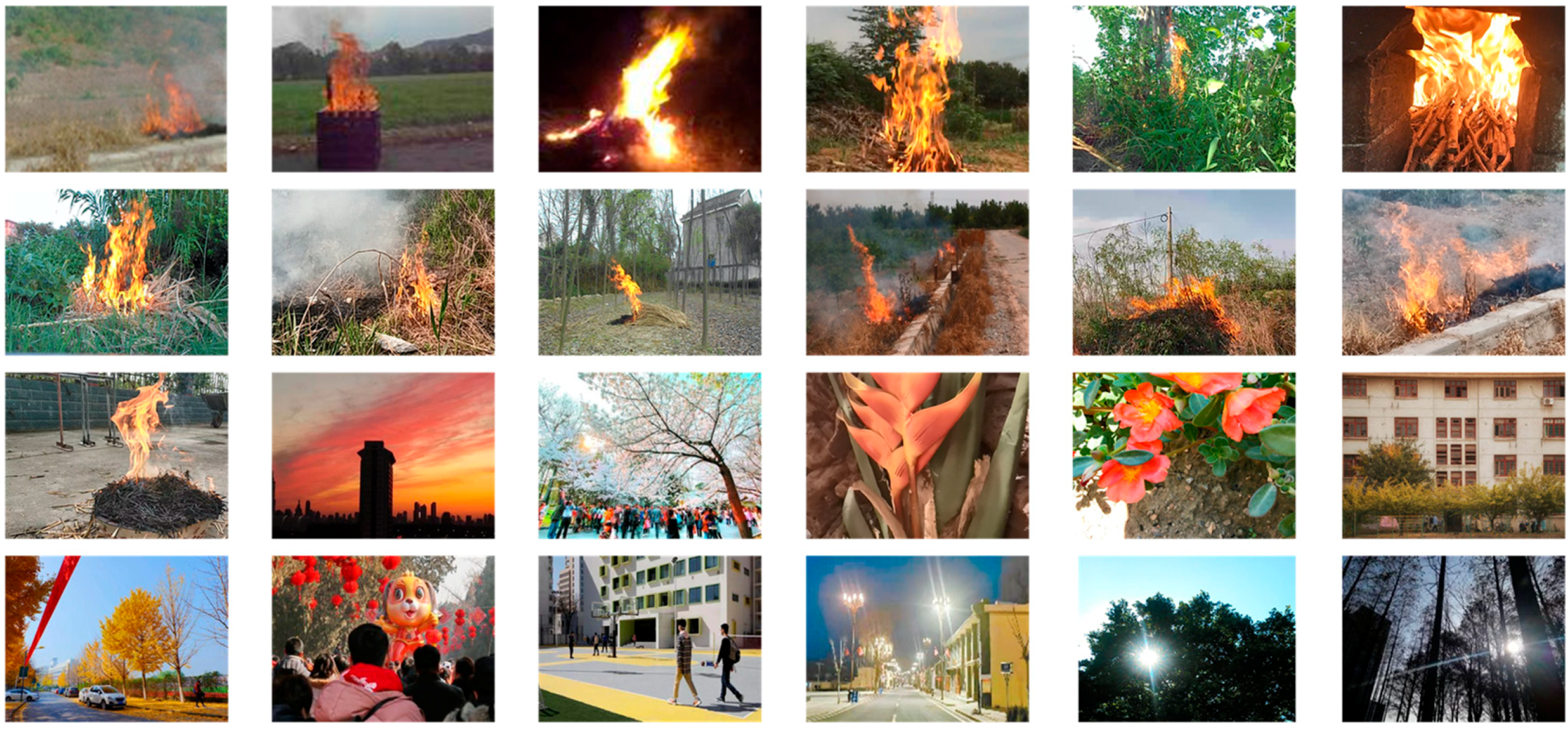
Training Datasets. Since the purpose of our algorithm is to find the flame regions from image sequences, we mainly use the datasets containing flame videos for training. As shown in Figure 5, we record flame videos from 13 different scenes and 11 flame-like videos, and we select a total of 4000 flame video sequences and 1200 flame-like video sequences to train the network. We randomly divide the video sequences of each scene into ten groups and select one group from each scene to compose the verification set. The remaining video sequences are used as the training set. Although the TSCNNFlame supports any size input, the size of the images in the training sets is resized to 400 × 400 in order to support multiple batches of training.
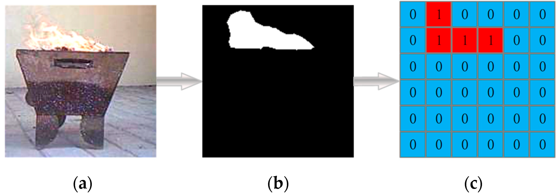
The labeling process of the training sets is shown in Figure 6. First, we set the values of the flame pixels to 255 and the values of the background pixels to 0 in Figure 6a to get the binary image shown Figure 6b. Then, we perform a convolution operation on the binary image. We divide one input image into small cells of the size 16 × 16 (but not limited to 16 × 16). We take the size of the convolution kernel as 16 × 16 × 1, the step size is 16, and all element values of the convolution kernel are 1. Thus, when the convolution kernel is sliding on the image, each convolution computation is equivalent to counting the number of flame pixels in each cell. Finally, a threshold is set to determine the label:
label ( x , y ) = { 1     e ( x , y ) s i z e 2 2   ×   255 0     e ( x , y ) < s i z e 2 2   ×   255 ,
where e ( x , y ) represents the value of each element after convolution, s i z e is the length of the cell of the size 16 × 16, and label ( x , y ) is the label value of a cell in Figure 6c. The value e ( x , y ) is equal to s i z e 2 2   ×   255 when flame pixels in a cell account for exactly half. So, the threshold is set to s i z e 2 2   ×   255 . The above formula indicates that this cell is labeled as the background region if the number of flame pixels is less than half of the pixels in the cell. Otherwise, this cell is recognized as the flame region.

4.2. Adaptive Adjustment of the Receptive Field

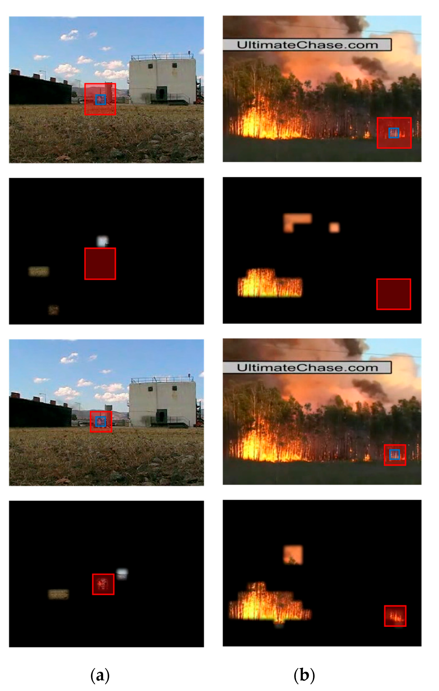
SKnet is used to adjust the size of the receptive fields when one flame video contains smaller flame regions than the corresponding receptive fields of the proposed network. To evaluate the ability, we select the challenging flame videos such as a small flame area captured on a distant view (shown in Figure 7a) or some small fragment-like flame regions (shown in Figure 7b). In the experiments, we compute the size of the receptive field using Equation (3) and Equation (4). In Figure 7, when the size of the flame block detected is about 20 × 20, the size of the receptive field is reduced from about 140 × 140 to 90 × 90 or so. As a result, the proportion of flame pixels in the receptive field increases, which decreases the missing rate. Therefore, the proposed scheme in the paper can automatically reduce the size of the receptive field to improve the capture ability of small flame areas.

4.3. Comparison of Recognition Performance

To better test the recognition performance of our proposed model, we select the public datasets widely used for evaluating flame detection methods as most of our testing sets. The public datasets are sourced from Foggia et al. [36] and the website https://github.com/steffensbola/furg-fire-dataset (accessed on 1 February 2021). We also record four challenging videos to evaluate the anti-interference performance of our model. We randomly intercepted 100 to 200 video blocks from each video, and each video block contains seven frames that are used as the input of the temporal stream of the proposed model.
For a comparison of our results with state-of-the-art methods, we selected a total of three related works, namely FCN, CNNFire, and DeepLab V3+. Both DeepLab V3+ and FCN are semantic segmentation networks with encoder–decoder structures, and the two models have been proved to have outstanding performance.

4.3.1. Comparison of Recognition Accuracy

We use dataset1 to evaluate the recognition accuracy. All the videos in dataset1 are from public datasets, as given in Figure 8. The videos in the dataset1 all contain flame objects, and the flame areas of each video account for a relatively large proportion of the video images.
Both F s c o r e and mean Intersection over Union ( m I o U ) are used to evaluate the performance of the four models. The I o U is an effective metric, and here, it is defined as the area of overlap between the detected flame region and the ground truth divided by the area of union between the detected flame region and the ground truth [37].
I o U = g r o u n d T r u t h   p r e d i c t i o n g r o u n d T r u t h p r e d i c t i o n
F s c o r e is the most used evaluation metric and is defined as the harmonic mean of precision and recall, taking into account the detected regions with true positives, false positives, and false negatives [37].
F s c o r e = 2   ×   p r e c i s i o n   ×   r e c a l l p r e c i s i o n + r e c a l l   ,
I o U and F s c o r e values range from 0 to 1, where these metric scores reach their best values at 1.
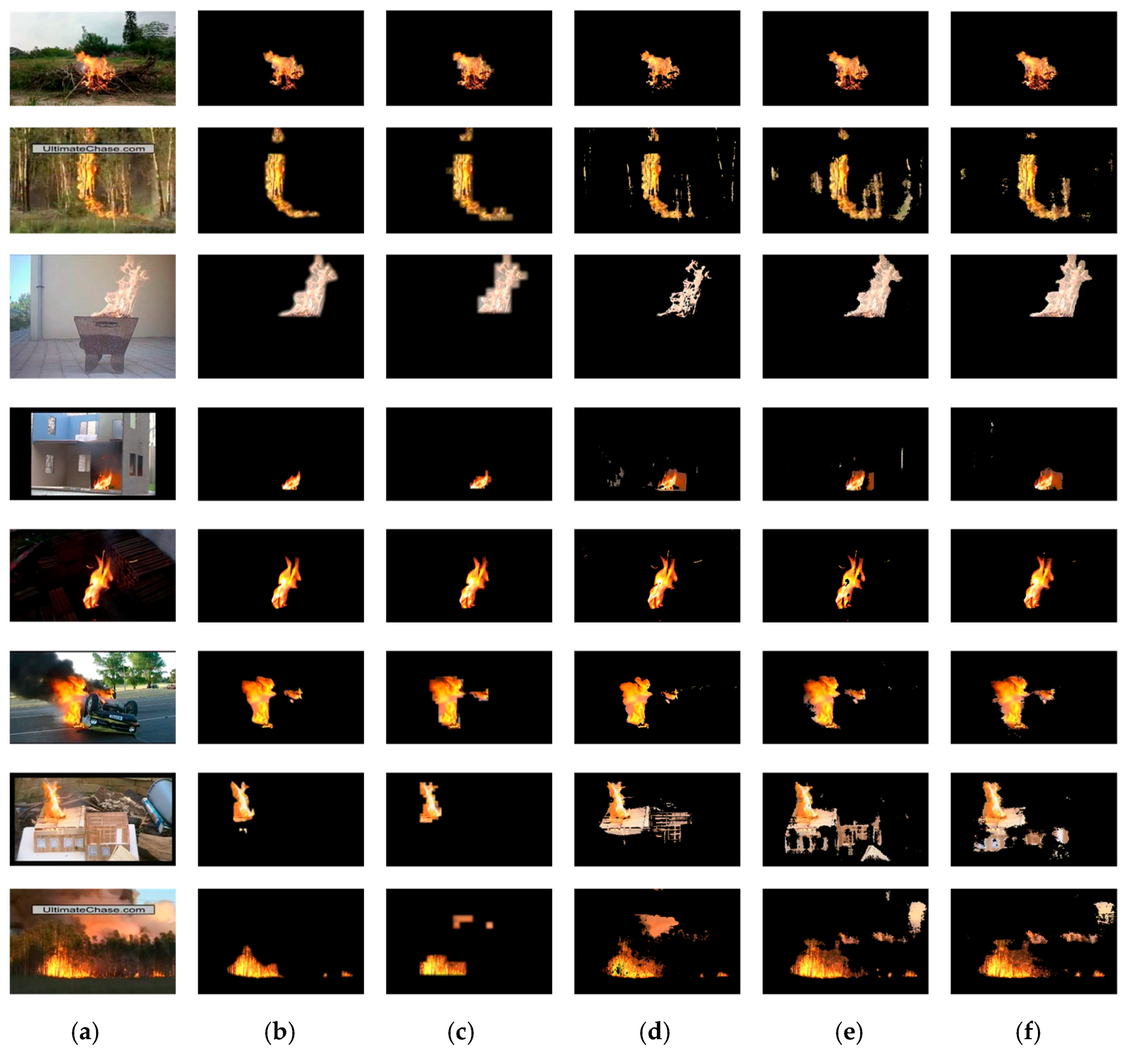
Table 2 and Table 3 show the F s c o r e and I o U of our model and three other models, respectively. As seen from the rightmost of Table 2 and Table 3, TSCNNFlame is superior to the other three models, no matter the F s c o r e or I o U . CNNFire designs special decision rules relying on the thresholds, which lead to the poor adaptability in generalization for various flame videos such as Video3, Video4, and Video7, as shown in Figure 9. FCN generates many more false positive pixels than TSCNNFlame if one video contains a large number of interference pixels, such as Video2 and Video7 shown in Figure 9. DeepLab V3+ still suffers from false detections and missing detections when one flame video such as Video4 contains the blurry contour of the flame region or multiple non-flame instances, which leads to low F s c o r e of Video7 in Table 2 and low I o U of Video2 in Table 3. TSCNNFlame adopts a dual-stream structure to supplement the lack of spatial features with frame difference features, so that compared with other methods, this method is more robust.
As shown in the third row (Video3) and the fifth row (Video5) in Figure 9, the edges of flame regions in the two videos look clear and have a lot of complex curvatures due to the simple background. For the two videos, TSCNNFlame has a lower F s c o r e and I o U value than the other three methods because using pixel blocks as the detection unit is unable to accurately extract the edges of the flame region, although we use Gaussian filtering to smooth the flame contours. However, the backgrounds of the two videos are relatively simple and do not contain flame-like flame objects. Combining Figure 9, Table 2 and Table 3, it can be seen that all the methods including TSCNNFlame can detect flame regions effectively. It is worth mentioning that the contour of the outer flame is often blurred due to the influence of a complex background, and thus, the detection error caused by the block detection can be generally ignored.

4.3.2. Comparison of Anti-Interference

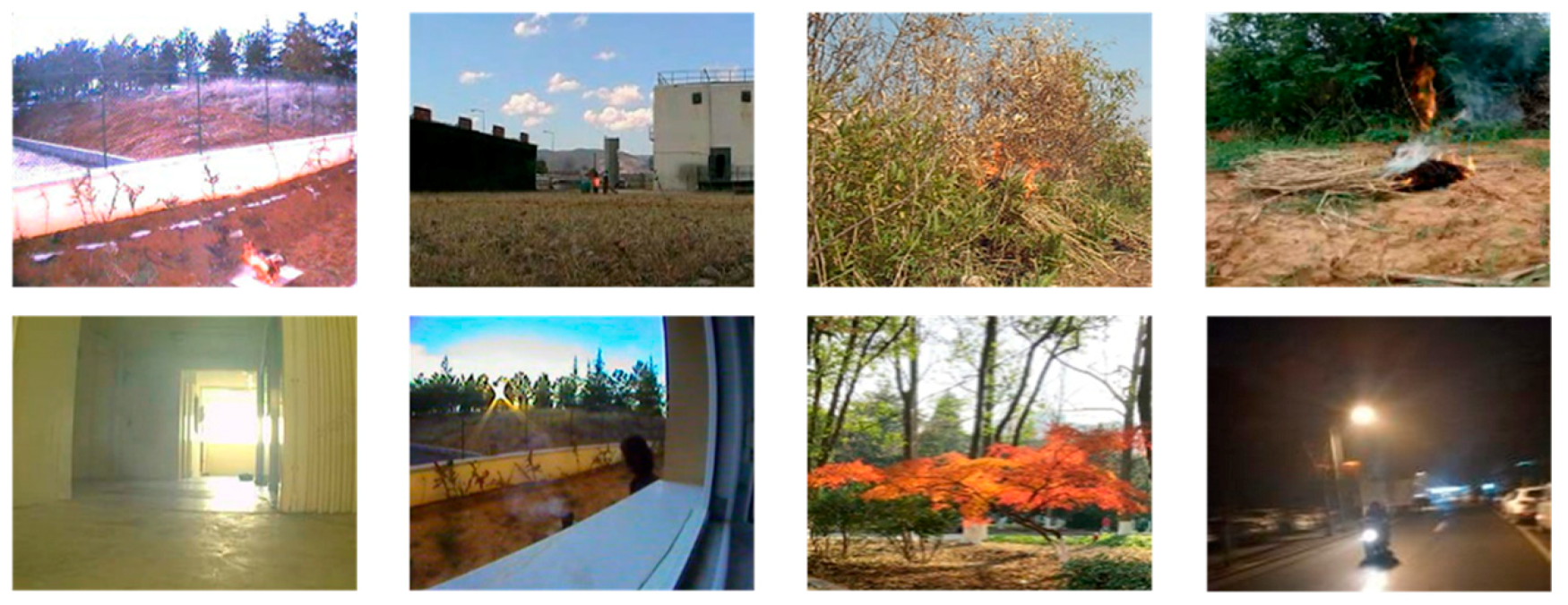
In this section, we evaluate the performance of anti-interference of our model using Dataset2, which is composed of eight challenging videos including four flame videos (shown in the top row of Figure 10) and four flame-like normal videos (shown in the bottom row of Figure 10). In Dataset2, the interference pixels in the flame images are much more than those of Dataset1 in Section 4.3.2. The two columns on the left in Figure 10 show four public videos from the website given in the first paragraph of Section 4.3, and the remaining four videos are recorded by us. As seen from Figure 11, compared with the other three methods, our method utilizes the temporal features to reduce the false detection rate of positive pixels because the static flame-like pixels are correctly detected as background pixels. Moreover, the SKnet block makes the receptive fields change with the portion of flame pixels in it, which helps increase the accuracy for positive pixel detection in the small flame region shown on the top row of Figure 11.
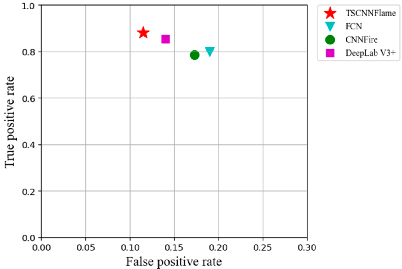
The Receiver Operating Characteristic (ROC) space [2] shows the relation between the false-positive rate and the true-positive rate. We compute the number of overlapping flame pixels in the detection maps and ground truth images, and we use that as true positives. Similarly, we also determine the number of non-overlapping flame pixels in the detection maps and take that as false positives. Figure 12 shows the ROC space on Datasets2 for the fourth method. As seen from Figure 12, our approach maintains a better balance between the true positive rate and the false positive rate than the other three methods.
The temporal stream in TSCNNFlame has a certain degree of interference suppression. In addition, TSCNNFlame uses 16 × 16 pixel blocks as the detection unit, and the receptive field size is smaller than other methods. So, in the process of convolution, the feature difference between adjacent pixel blocks is relatively large, and it is not prone to batch continuous misdetection.

4.4. Running Time

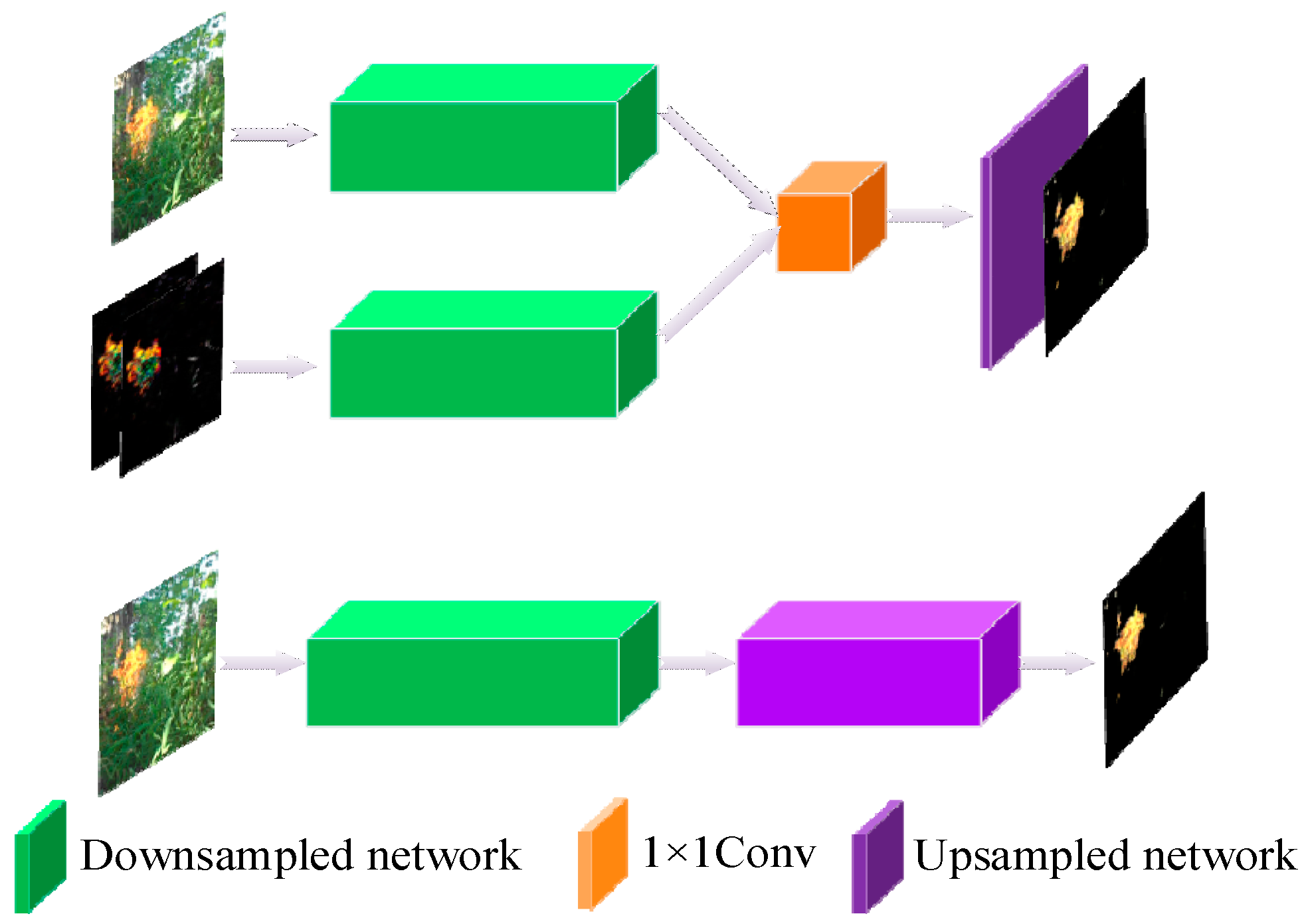
TSCNNFlame adopts the idea of directly classifying candidate regions. As shown in Figure 13, compared with encoder–decoder structures such as FCN and DeepLab V3+, TSCNNFlame removes the decoder-based complex structure, reduces the number of network layers, and increases the frame difference input stream. The architecture of the temporal stream in TSCNNFlame is the same as that of the spatial stream, and thus, the parallel calculation in the processor makes the running time of the network much less than the structures of encoder–decoder serial networks.
We use Fps (Frames per second) to evaluate the detecting speed of the four compared methods. The testing data used for all four methods are the same video sequences from Dataset1 and Dataset2. As shown in Table 4, the detection speed of TSCNNFlame is much faster than FCN and DeepLab V3+, and it is nearly comparable with CNNFire that has a single-stream structure and no upsampling calculation. However, as shown in Table 2 and Table 3 and Figure 9 and Figure 11, TSCNNFlame has higher detection accuracy than CNNFire.

5. Conclusions and Limitations

In this paper, we proposed a novel CNN architecture for flame region detection. We take two main measures to achieve a good compromise between accuracy and efficiency. One measure is the lightweight network but the fusion of temporal–spatial features. The other is the SK-Shuffle block that adaptively adjusts receptive fields while reducing the network parameters, which has great significance for some very small flame areas captured on a distant view or some small fragment-like flame regions. The proposed method achieves comparable or superior performance with state-of-art methods but is less time-consuming. In the experimental results, it achieves an average F s c o r e of 82.95%, an average I o U of 82.54%, and a detection speed of 35 F p s . In particular, our method is outstanding for the videos containing a large number of flame-like interference objects.
Although the proposed method achieves a pleasant trade-off between flame region segmentation accuracy and efficiency, sometimes, there are errors inevitably when the edge of one flame region has a changeable and complex curvature due to the block-wise detection scheme. Future studies may segment one frame image into small super pixel blocks instead of fixed size blocks. The pixels in one super pixel block have similar characteristics, which may help to improve the accuracy.

Author Contributions

Conceptualization, P.L. and Y.Z.; methodology, P.L.; software, P.L.; validation, Y.Z. and Y.X.; formal analysis, Y.X.; investigation, P.L.; resources, Y.Z.; data curation, Y.X.; writing—original draft preparation, P.L.; writing—review and editing, Y.Z.; visualization, Y.X.; supervision, Y.Z.; project administration, Y.Z.; funding acquisition, Y.X. All authors have read and agreed to the published version of the manuscript.

Funding

This research was funded by the National Natural Science Fund, grant number No.31200496.

Data Availability Statement

The data presented in this study are available on request from the corresponding author.

Conflicts of Interest

The authors declare no conflict of interest. The funders had no role in the design of the study; in the collection, analyses, or interpretation of data; in the writing of the manuscript, or in the decision to publish the results.

References

  1. Çelik, T.; Demirel, H. Fire Detection in Video Sequences Using a Generic Color Model. Fire Saf. J. 2009, 44, 147–158. [Google Scholar] [CrossRef]
  2. Chino, D.Y.; Avalhais, L.P.; Rodrigues, J.F.; Traina, A.J. Detection of Fire in Still Images by Integrating Pixel Color and Texture Analysis. In Proceedings of the 2015 28th SIBGRAPI Conference on Graphics, Patterns and Images, Salvador, Brazil, 26–29 August 2015; pp. 95–102. [Google Scholar]
  3. Mueller, M.; Karasev, P.; Kolesov, I.; Tannenbaum, A. Optical Flow Estimation for Flame Detection in Videos. IEEE Trans. Image Process. 2013, 22, 2786–2797. [Google Scholar] [CrossRef] [PubMed] [Green Version]
  4. Di Lascio, R.; Greco, A.; Saggese, A.; Vento, M. Improving fire detection reliability by a combination of videoanalytics. In Proceedings of the International Conference Image Analysis and Recognition; Springer: Cham, Switzerland, 2014; pp. 477–484. [Google Scholar]
  5. Dimitropoulos, K.; Barmpoutis, P.; Grammalidis, N. Spatio-temporal flame modeling and dynamic texture analysis for automatic video-based fire detection. IEEE Trans. Circuits Syst. Video Technol. 2015, 25, 339–351. [Google Scholar] [CrossRef]
  6. Li, Q.; Yuan, P.; Liu, X.; Zhou, H. Street tree segmentation from mobile laser scanning data. Int. J. Remote. Sens. 2020, 41, 7145–7162. [Google Scholar] [CrossRef]
  7. Kim, J.-H.; Kima, B.-G.; Roy, P.P.; Jeong, D.-M. Efficient Facial Expression Recognition Algorithm Based on Hierarchical Deep Neural Network Structure. IEEE Access 2019, 7, 41273–41285. [Google Scholar] [CrossRef]
  8. Frizzi, S.; Kaabi, R.; Bouchouicha, M.; Ginoux, J.-M.; Moreau, E.; Fnaiech, F. Convolutional Neural Network for Video Fire and Smoke Detection. In Proceedings of the IECON 2016—42nd Annual Conference of the IEEE Industrial Electronics Society, Florence, Italy, 23–26 October 2016; pp. 877–882. [Google Scholar]
  9. Sharma, J.; Granmo, O.-C.; Goodwin, M.; Fidje, J.T. Deep Convolutional Neural Networks for Fire Detection in Images. In Proceedings of the International Conference on Engineering Applications of Neural Networks; Springer: Cham, Switzerland, 2017; pp. 183–193. [Google Scholar]
  10. Zhong, Z.; Wang, M.; Shi, Y.; Gao, W. A Convolutional Neural Network-Based Flame Detection Method in Video Sequence. Signal Image Video Process. 2018, 12, 1619–1627. [Google Scholar] [CrossRef]
  11. Yu, N.; Chen, Y. Video Flame Detection Method Based on TwoStream Convolutional Neural Network. In Proceedings of the 2019 IEEE 8th Joint International Information Technology and Artificial Intelligence Conference (ITAIC), Chongqing, China, 24–26 May 2019. [Google Scholar]
  12. Muhammad, K.; Ahmad, J.; Lv, Z.; Bellavista, P.; Yang, P.; Baik, S.W. Efficient Deep CNN-Based Fire Detection and Localization in Video Surveillance Applications. IEEE Trans. Syst. Man, Cybern. Syst. 2018, 49, 1419–1434. [Google Scholar] [CrossRef]
  13. Chen, T.-H.; Wu, P.-H.; Chiou, Y.-C. An Early Fire-Detection Method Based on Image Processing. In Proceedings of the 2004 International Conference on Image Processing, 2004. ICIP ’04, Singapore, 24–27 October 2004; Volume 3, pp. 1707–1710. [Google Scholar]
  14. Wang, H.; Finn, A.; Erdinc, O.; Vincitore, A. Spatial-Temporal Structural and Dynamics Features for Video Fire Detection. In Proceedings of the 2013 IEEE Workshop on Applications of Computer Vision (WACV), Clearwater Beach, FL, USA, 15–17 January 2013; pp. 513–519. [Google Scholar]
  15. Töreyin, B.U.; Dedeoğlu, Y.; Güdükbay, U.; Cetin, A.E. Computer Vision Based Method for Real-Time Fire and Flame Detection. Pattern Recognit. Lett. 2006, 27, 49–58. [Google Scholar] [CrossRef] [Green Version]
  16. Zhang, Q.; Xu, J.; Xu, L.; Guo, H. Deep Convolutional Neural Networks for Forest Fire Detection. In Proceedings of the 2016 International Forum on Management, Education and Information Technology Application; Atlantis Press: Paris, France, 2016; pp. 568–575. [Google Scholar]
  17. Muhammad, K.; Khan, S.; Elhoseny, M.; Ahmed, S.H.; Baik, S.W. Efficient Fire Detection for Uncertain Surveillance Environment. IEEE Trans. Ind. Inform. 2019, 15, 3113–3122. [Google Scholar] [CrossRef]
  18. Dunnings, A.J.; Breckon, T.P. Experimentally Defined Convolutional Neural Network Architecture Variants for Non-Temporal Real-Time Fire Detection. In Proceedings of the 2018 25th IEEE International Conference on Image Processing (ICIP), Athens, Greece, 7–10 October 2018; pp. 1558–1562. [Google Scholar]
  19. Chaoxia, C.; Shang, W.; Zhang, F. Information-Guided Flame Detection Based on Faster R-CNN. IEEE Access 2020, 8, 58923–58932. [Google Scholar] [CrossRef]
  20. Kim, B.; Lee, J. A Video-Based Fire Detection Using Deep Learning Models. Appl. Sci. 2019, 9, 2862. [Google Scholar] [CrossRef] [Green Version]
  21. Li, P.; Zhao, W. Image Fire Detection Algorithms Based on Convolutional Neural Networks. Case Stud. Therm. Eng. 2020, 19, 100625. [Google Scholar] [CrossRef]
  22. Muhammad, K.; Ahmad, J.; Mehmood, I.; Rho, S.; Baik, S.W. Convolutional Neural Networks Based Fire Detection in Surveillance Videos. IEEE Access 2018, 6, 18174–18183. [Google Scholar] [CrossRef]
  23. Long, J.; Shelhamer, E.; Darrell, T. Fully Convolutional Networks for Semantic Segmentation. In Proceedings of the 2015 IEEE Conference on Computer Vision and Pattern Recognition (CVPR), Boston, MA, USA, 7–12 June 2015; pp. 3431–3440. [Google Scholar]
  24. He, K.; Gkioxari, G.; Dollar, P.; Girshick, R. Mask R-CNN. In Proceedings of the 2017 IEEE International Conference on Computer Vision (ICCV), Venice, Italy, 22–29 October 2017; pp. 2980–2988. [Google Scholar]
  25. Chen, L.-C.; Papandreou, G.; Kokkinos, I.; Murphy, K.; Yuille, A.L. Semantic Image Segmentation with Deep Convolutional Nets and Fully Connected CRFs. In Proceedings of the International Conference on Learning Representations, San Diego, CA, USA, 7–9 May 2015. [Google Scholar]
  26. Chen, L.-C.; Papandreou, G.; Kokkinos, I.; Murphy, K.; Yuille, A.L. DeepLab: Semantic Image Segmentation with Deep Convolutional Nets, Atrous Convolution, and Fully Connected CRFs. arXiv 2016, arXiv:1606.00915. [Google Scholar] [CrossRef] [PubMed]
  27. Chen, L.-C.; Papandreou, G.; Schroff, F.; Adam, H. Rethinking Atrous Convolution for Semantic Image Segmentation. arXiv 2017, arXiv:1706.05587. [Google Scholar]
  28. Chen, L.-C.; Zhu, Y.; Papandreou, G.; Schroff, F.; Adam, H. Encoder-Decoder with Atrous Separable Convolution for Semantic Image Segmentation. In Proceedings of the European Conference on Computer Vision (ECCV), Munich, Germany, 8–14 September 2018; pp. 833–851. [Google Scholar]
  29. Benitez-Garcia, G.; Prudente-Tixteco, L.; Castro-Madrid, L.C.; Toscano-Medina, R.; Olivares-Mercado, J.; Sanchez-Perez, G.; Villalba, L.J.G. Improving Real-Time Hand Gesture Recognition with Semantic Segmentation. Sensors 2021, 21, 356. [Google Scholar] [CrossRef]
  30. Li, X.; Wang, W.; Hu, X.; Yang, J. Selective Kernel Networks. In Proceedings of the 2019 IEEE/CVF Conference on Computer Vision and Pattern Recognition (CVPR), Long Beach, CA, USA, 16–20 June 2019; pp. 510–519. [Google Scholar]
  31. Dumoulin, V.; Visin, F. A Guide to Convolution Arithmetic for Deep Learning. arXiv 2016, arXiv:1603.07285. [Google Scholar]
  32. Howard, A.G.; Zhu, M.; Chen, B.; Kalenichenko, D.; Wang, W.; Weyand, T.; Andreetto, M.; Adam, H. MobileNets: Efficient Convolutional Neural Networks for Mobile Vision Applications. arXiv 2017, arXiv:1704.04861. [Google Scholar]
  33. Sandler, M.; Howard, A.; Zhu, M.; Zhmoginov, A.; Chen, L.-C. MobileNetV2: Inverted Residuals and Linear Bottlenecks. In Proceedings of the 2018 IEEE/CVF Conference on Computer Vision and Pattern Recognition, Salt Lake City, UT, USA, 18–23 June 2018; pp. 4510–4520. [Google Scholar]
  34. Zhang, X.; Zhou, X.; Lin, M.; Sun, J. ShuffleNet: An Extremely Efficient Convolutional Neural Network for Mobile Devices. arXiv 2017, arXiv:1707.01083. [Google Scholar]
  35. Ma, N.; Zhang, X.; Zheng, H.-T.; Sun, J. ShuffleNet V2: Practical Guidelines for Efficient CNN Architecture Design. In Proceedings of the European Conference on Computer Vision (ECCV), Munich, Germany, 8–14 September 2018; pp. 122–138. [Google Scholar]
  36. Foggia, P.; Saggese, A.; Vento, M. Real-Time Fire Detection for Video-Surveillance Applications Using a Combination of Experts Based on Color, Shape, and Motion. IEEE Trans. Circuits Syst. Video Technol. 2015, 25, 1545–1556. [Google Scholar] [CrossRef]
  37. Barmpoutis, P.; Stathaki, T.; Dimitropoulos, K.; Grammalidis, N. Early Fire Detection Based on Aerial 360-Degree Sensors, Deep Convolution Neural Networks and Exploitation of Fire Dynamic Textures. Remote. Sens. 2020, 12, 3177. [Google Scholar] [CrossRef]
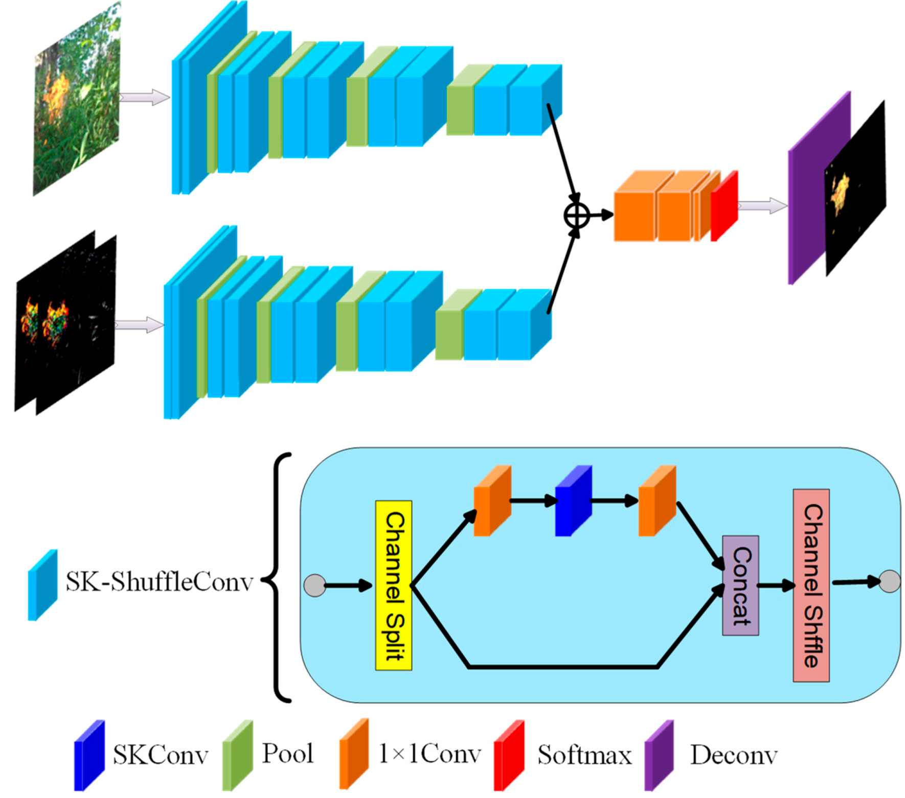
Figure 1. Overview of the proposed network for flame region detection.
Symmetry 13 00397 g001
Figure 2. The two-branch structure of selective kernel (SK) convolution.
Symmetry 13 00397 g002
Figure 3. Representation of receptive field, detection area, and detection result.
Symmetry 13 00397 g003
Figure 4. Fusion of SK convolution and ShuffleNet V2 structure. (a) ShuffleNet V2 block; (b) SK-ShuffleConv.
Symmetry 13 00397 g004
Figure 5. The sample of the training set.
Symmetry 13 00397 g005
Figure 6. Training set production process. (a) Original image; (b) Ground truth; (c) Training label.
Symmetry 13 00397 g006
Figure 7. Comparison of the adaptive adjustment of a receptive field with a fixed receptive field, First row: input image with a fixed receptive field; Second row: output result with a fixed receptive field; Third row: input image with an adjusted receptive field; Fourth row: output result with a fixed receptive field. (a) Sample with small flame area; (b) Sample with small fragment-like flame regions.
Symmetry 13 00397 g007
Figure 8. Sample images from Dataset1.
Symmetry 13 00397 g008
Figure 9. Output of each method from Dataset1, From top row to bottom row, Video1 to Video8, respectively. (a) Input frame; (b) Ground truth; (c) TSCNNFlame; (d) CNNFire [12]; (e) FCN [23]; (f) DeepLab V3+ [28]).
Symmetry 13 00397 g009
Figure 10. Sample images of the challenging videos from Dataset2.
Symmetry 13 00397 g010
Figure 11. Output of each methods with a frame with fire from Dataset2. (a) Input frame; (b) TSCNNFlame; (c) CNNFire [12]; (d) FCN [23]; (e) DeepLab V3+ [28]).
Symmetry 13 00397 g011
Figure 12. Receiver Operating Characteristic (ROC) space on Dataset2.
Symmetry 13 00397 g012
Figure 13. Comparison of two-stream structure and encoder–decoder structure.
Symmetry 13 00397 g013
Table 1. The complete network structure of two-stream convolutional neural network for flame region detection (TSCNNFlame).
InputSpatial stream/Temporal StreamOutput
W × H × 3[3 × 3, 64, Stride:1] × 2W × H × 64
W × H × 32 × 2 max pool, stride 2W/2 × H/2 × 64
W/2 × H/2 × 64 [ 1 × 1 ,   128 S K ( 3 × 3 5 × 5 ) ,   128 1 × 1 ,   128 ] × 2W/2 × H/2 × 128
W/2 × H/2 × 1282 × 2 max pool, stride 2W/4 × H/4 × 128
W/4 × H/4 × 128 [ 1 × 1 ,   256 S K ( 3 × 3 5 × 5 ) , 256 1 × 1 ,   256 ] × 2W/4 × H/4 × 256
W/4 × H/4 × 2562 × 2 max pool, stride 2W/8 × H/8 × 256
W/8 × H/8 × 256 [ 1 × 1 ,   512 S K ( 3 × 3 5 × 5 ) , 512 1 × 1 ,   512 ] × 2W/8 × H/8 × 512
W/16 × H/16 × 5122 × 2 max pool, stride 2W/16 × H/16 × 512
W/16 × H/16 × 512 [ 1 × 1 , 512 S K ( 1 × 1 3 × 3 5 × 5 ) , 512 1 × 1 ,   512 ] × 2W/16 × H/16 × 512
W/16 × H/16 × 512fusionW/16 × H/16 × 1024
W/16 × H/16 × 10241 × 1, 1024, Stride:1W/16 × H/16 × 1024
W/16 × H/16 × 10241 × 1, 512, Stride:1W/16 × H/16 × 512
W/16 × H/16 × 5121 × 1, 2, Stride:1, softmaxW/16 × H/16 × 2
Table 2. F s c o r e of various fire detection methods for Dataset1.
Video1Video2Video3Video4Video5Video6Video7Video8Avg
FCN86.2%66.5%90.8%76.7%89.8%89.4%63.1%71.5%79.25%
CNNFire82.3%68.9%85.4%72.2%92.1%87.5%69.3%76.4%79.26%
DeepLab V3+87.4%74.2%91.3%78.7%84.3%90.7%63.7%74.1%80.55%
TSCNNFlame87.6%75.4%89.2%83.5%85.2%91.1%73.0%78.6%82.95%
Table 3. Intersection over Union ( I o U ) of various fire detection methods for Dataset1.
Video1Video2Video3Video4Video5Video6Video7Video8Avg
FCN75.3%64.9%92.2%74.7%90.9%84.0%70.2%69.3%77.69%
CNNFire71.0%62.1%81.7%77.3%93.5%82.2%78.4%72.2%77.30%
DeepLab V3+83.4%58.1%92.8%79.5%91.3%85.2%70.7%71.1%79.01%
TSCNNFlame84.7%71.2%88.5%84.7%89.8%85.9%82.1%73.4%82.54%
Table 4. Fps (Frames per second) of various fire detection methods.
MethodFps
FCN5
CNNFire39
DeepLab V3+14
TSCNNFlame35
Publisher’s Note: MDPI stays neutral with regard to jurisdictional claims in published maps and institutional affiliations.